Cancelation of dispersion and temporal modulation with non-entangled frequency-correlated photons

Abstract

The observation of the so-called dispersion cancelation and temporal phase modulation of paired photons is generally attributed to the presence of frequency entanglement between two frequency anticorrelated photons. In this paper, it is shown that by introducing the appropriate amount of chromatic dispersion or phase modulation between non-entangled photons, it is also possible to observe these effects. Indeed, it is found that the relevant characteristic for the observation of dispersion cancelation or the cancelation of temporal phase modulation is the presence of certain frequency correlations between the photons.

I Introduction

The theory of quantum coherence glauber1963 ; glauber2006 describes the temporal and frequency characteristics of a stream of photons through a hierarchy of correlation functions. In particular, the second-order correlation function determines the probability to detect a photon at a certain location and instant time in coincidence with a companion photon at another location and time. This magnitude is often used to test the quantum or classical nature of a light source mandel_book . For instance, the normalized correlations of classical fields (i.e., fields with a positive $P$-representation) obey certain inequalities, whose violation constitutes an unequivocal signature of the non-classical properties of the light kimble .

A particular type of correlation between photons is entanglement. Paired photons that show frequency entanglement can be generated by means of the process of spontaneous parametric downconversion (SPDC). Interestingly, in an SPDC process, classical-like features of the fluctuations of the beams coexist with the strong nonclassical photon-pair correlations loudon .

Two important effects have been attributed to the existence of frequency entanglement and its demonstration have made use of the correlations existing between signal and idler photons generated in SPDC. The first effect is dispersion cancelation franson1992 ; gisin1998 ; kim2009 , which is observed in the temporal domain. Briefly, if the signal and idler photons generated in SPDC pumped by a continuous-wave (CW) beam are sent through two separate dispersive optical elements, such as single-mode fibers, with corresponding group-delay-dispersion (GDD) coefficients $\Phi_{1}$ and $\Phi_{2}$, the temporal width of the second-order correlation function increases as $(\Phi_{1}+\Phi_{2})^{2}$, in a similar way to the broadening of a pulse that propagates in an optical fiber due to chromatic dispersion valencia2002 . So, if the GDD parameters of both dispersive media are identical but of opposite sign, the broadening of the second-order correlation function can be suppressed. This is in contrast to the case where two identical broadband coherent light pulses propagate through two dispersive media such as single-mode optical fibers. In this case, the cross-correlation width broadens as $(\Phi_{1}^{2}+\Phi_{2}^{2})$ and therefore the cancelation of the dispersion effects is never possible franson1992 .

The second effect is remote temporal modulation of entangled photons harris2008 ; harris2009 , which is observed in the frequency domain. For a CW-pumped SPDC process, the detection of a signal photon at frequency $\omega_{1}$ would only coincide with the detection of an idler photon at frequency $\omega_{2}$, given that $\omega_{1}+\omega_{2}=2\omega_{0}$, where $2\omega_{0}$ is the frequency of the CW pump beam. When synchronously driven temporal modulators are placed in the signal and idler paths, respectively, new frequency correlations appear. In a similar manner to dispersion cancelation, if the two identical modulators are driven in opposite phase, their global effect is to negate each other and the spectral correlations appear as those when there are no phase modulators present.

It becomes of fundamental relevance to determine whether these effects are due to the classical or the quantum-like behavior of the SPDC source. Several authors have shown that similar dispersion cancelation effects can be obtained with non-entangled light victor2009 ; shapiro2010 . In particular, the work in victor2009 considers classical thermal light equally split in two dispersive arms and demonstrates that the broadening of the second-order correlation function increases as $(\Phi_{1}-\Phi_{2})^{2}$, so that it remains unaffected if $\Phi_{1}=\Phi_{2}$. Later, the work in shapiro2010 shows that by introducing a phase conjugator element in one arm of the intensity interferometer (producing a Gaussian-state light source), the broadening of the correlation function increases as $(\Phi_{1}+\Phi_{2})^{2}$, similar to the signal-idler photon pairs from SPDC, and thus the same dispersion compensation rules apply.

In this work, we provide new insights into the effects of dispersion cancelation and temporal modulation applying the Heisenberg picture. This formalism allows us to include the case of multiphoton pair generation in a straightforward way, and thus to calculate all relevant coherence functions (signal-signal and signal-idler correlations). Two important findings are revealed: First, there is a background term in the second-order correlation function for all types of correlations, but the signal-to-background ratio for signal-signal correlations is lower than for the signal-idler correlations franson2009 ; franson2010 . Second and more importantly, dispersion cancelation and temporal modulation can also be observed with the correlation existing among photons from an individual beam of SPDC (i.e., either signal-signal or idler-idler), which do not show entanglement. This last point illustrates that it is the existence of certain frequency correlations between photons, rather than the entanglement, that is the key enabling factor that allows the observation of dispersion cancelation and remote temporal modulation.

II Quantum description of the light generated in Spontaneous Parametric Downconversion

The effects studied in this work, i.e., remote dispersion cancelation and cancelation of temporal modulation are observed in the corresponding second-order correlation functions. To calculate these magnitudes one needs to establish the dependence of the creation and annihilation operators with the physical parameters set by the SPDC process. In this section, we review the quantum theory of the SPDC process pumped by a CW pump and establish this dependence.

Let us consider degenerate SPDC produced by a CW plane-wave pump with a central frequency $2\omega_{0}$ in a crystal of length $L$ and nonlinear coefficient $\chi^{(2)}$. Within the Heisenberg formalism, the propagation equations describing the evolution of the signal and idler creation $\tilde{a}_{s,i}^{{\dagger}}(\omega_{0}+\Omega)$ and annihilation $\tilde{a}_{s,i}(\omega_{0}+\Omega)$ operators can be written as loudon ; barak

$$\frac{\partial\tilde{a}_{s}\left(z,\Omega\right)}{\partial z} = \sigma\tilde{a}_{i}^{{\dagger}}\left(z,-\Omega\right)\exp\left[i\Delta(\Omega)z\right],$$ (1)

$$\frac{\partial\tilde{a}_{i}\left(z,\Omega\right)}{\partial z} = \sigma\tilde{a}_{s}^{{\dagger}}\left(z,-\Omega\right)\exp\left[i\Delta(\Omega)z\right],$$ (2)

where $\Omega$ is the frequency deviation from the central frequency $\omega_{0}$, $\Delta\left(\Omega\right)=k_{p}^{0}-k_{s}\left(\Omega\right)-k_{i}\left(-\Omega\right)$ is the phase matching function, $\sigma$ is a constant parameter proportional to the number of pump photons traversing the nonlinear crystal, $k_{j}(\Omega)=(\omega_{0}+\Omega)n_{j}/c$ denotes the signal and idler wavenumbers, with $n_{j}$ being the refractive index at the corresponding central frequencies, $k_{p}^{0}=2\omega_{0}n_{p}/c$ the wavenumber of the pump beam and $c$ the speed of light in a vacuum.

Solving Eqs. (1) and (2) and writing $\tilde{a}_{s}(z,\Omega)$ and $\tilde{a}_{i}(z,\Omega)$ in terms of the vacuum field operators at the input face of the nonlinear crystal, $b_{s}(\Omega)$ and $b_{i}(\Omega)$, we obtain navez ; brambilla

$$\tilde{a}_{s}(z,\Omega) = U(z,\Omega)b_{s}(\Omega)+V(z,\Omega)b_{i}^{\dagger}(-\Omega),$$ (3)

$$\tilde{a}_{i}(z,\Omega) = U(z,\Omega)b_{i}(\Omega)+V(z,\Omega)b_{s}^{\dagger}(-\Omega)$$ (4)

with

$$U(z,\Omega) = \exp\left[\frac{i\Delta(\Omega)z}{2}\right]\left\{\cosh\left[\Gamma(\Omega)z\right]\right.$$ (5)

$$\left.-\frac{i\Delta(\Omega)}{2\Gamma(\Omega)}\,\sinh\left[\Gamma(\Omega)z\right]\right\},$$

$$V(z,\Omega) = -\frac{i\sigma}{\Gamma(\Omega)}\exp\left[i\frac{\Delta(\Omega)z}{2}\right]$$ (6)

$$\times\sinh\left[\Gamma(\Omega)z\right],$$

where $\Gamma(\Omega)=(|\sigma|^{2}-\Delta^{2}(\Omega)/4)^{1/2}$ and $\sigma$ is the nonlinear coefficient of the medium.

From these results, we can calculate the required correlations in the temporal and frequency domains. We will refer to the second-order coherence function between signal and idler photons as to interbeam correlations. Analogously, we will refer to the second-order coherence function between signal-signal, or idler-idler, streams of photons as to intrabeam correlations. We will make use of the commutation rules $[b_{j}(\Omega_{1}),\,b_{k}(\Omega_{2})]=\delta(\Omega_{1}-\Omega_{2})\delta_{jk}$, where $\delta_{jk}$ is the Kronecker’s delta and $(j,k)=(s,i)$.

In particular, for the effect of dispersion cancelation, two quantities are of interest. For the interbeam second-order correlations, we have

$$G^{(2)}_{\textrm{inter}}(\tau)=\langle a_{s}^{\dagger}(t)a_{i}^{\dagger}(t+\tau)a_{i}(t+\tau)a_{s}(t)\rangle.$$ (7)

Here, the operators $a_{s,i}(t)$ form a Fourier transform pair with the creation operators $\tilde{a}_{s,i}(\Omega)$. The above magnitude is related to the probability of detecting a signal photon at time $t$ in coincidence with an idler photon at $t+\tau$. For the intrabeam correlations, the corresponding magnitude is

$$G^{(2)}_{\textrm{intra}}(\tau)=\langle a_{s}^{\dagger}(t)a_{s}^{\dagger}(t+\tau)a_{s}(t+\tau)a_{s}(t)\rangle,$$ (8)

where signal photons have been arbitrarily chosen. This function provides the probability of detecting a signal photon in coincidence with another signal photon at $t+\tau$.

Recent experiments suggest blauensteiner that intrabeam correlations in SPDC can be measured when high-power CW beams are used to pump the nonlinear crystal. Then the intrabeam higher-order correlations show classical-like features similar to thermal light yurke . In such a case, the interbeam correlations must be also adequately accounted for to include the multiphoton pair effects.

For the effects of cancelation of temporal modulation, the relevant second-order correlation functions are calculated in the spectral domain. In particular, for the interbeam photon correlations, one has

$$\tilde{G}^{(2)}_{\textrm{inter}}(\Omega_{1},\Omega_{2})=\langle\tilde{a}_{s}^{\dagger}(\Omega_{1})\tilde{a}_{i}^{\dagger}(\Omega_{2})\tilde{a}_{i}(\Omega_{2})\tilde{a}_{s}(\Omega_{1})\rangle,$$ (9)

which determines the probability of detecting a signal photon at frequency $\Omega_{1}$ in coincidence with an idler photon at frequency $\Omega_{2}$. Analogously, we consider the intrabeam second-order correlation function

$$\tilde{G}^{(2)}_{\textrm{intra}}(\Omega_{1},\Omega_{2})=\langle\tilde{a}_{s}^{\dagger}(\Omega_{1})\tilde{a}_{s}^{\dagger}(\Omega_{2})\tilde{a}_{s}(\Omega_{2})\tilde{a}_{s}(\Omega_{1})\rangle,$$ (10)

which establishes the probability of detecting in coincidence two signal photons, one at frequency $\Omega_{1}$ and the other at $\Omega_{2}$.

III Interbeam configuration: Cancelation of dispersion and temporal modulation in the multiphoton regime

In this section, we calculate the change in the interbeam correlations, $G^{(2)}_{\textrm{inter}}(\tau)$ and $G^{(2)}_{\textrm{inter}}(\Omega_{1},\Omega_{2})$, when the photons propagate through the optical systems corresponding to dispersion and temporal modulation cancelations, respectively. The goal of this study is to extend the previous theoretical results franson1992 ; harris2008 to the case in which multiphoton pairs are generated in the SPDC process.

In the interbeam configuration, signal and idler photons are separated (see Fig. 1), following afterwards paths $1$ and $2$. This arrangement can be achieved by generating SPDC photons that propagate in different directions (noncollinear type I) or that show orthogonal polarizations (collinear type II) and are divided by a polarizing beam splitter.

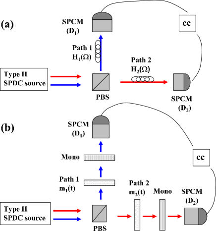
Figure 1: (Color online) General configurations for observing interbeam correlations in (a) the temporal domain and (b) the frequency domain. PBS: Polarizing beam splitter; SPCM: Single photon counting module; cc: coincidence counting; Mono: Monochromator. In (a) there are two single-mode optical fibers in paths $1$ and $2$ with transfer functions $H_{1}(\Omega)$ and $H_{2}(\Omega)$, respectively. In (b), there are two temporal phase modulators with transfer functions $m_{1}(t)$ and $m_{2}(t)$. Red and blue lines describe photons with orthogonal polarizations.

III.1 Dispersion cancelation in the interbeam configuration

Let us start by considering remote dispersion cancelation. As depicted in Fig. 1(a), before reaching the detectors, the signal photons traverse path $1$, with dispersive transfer function $H_{1}(\omega)$, and the idler photons traverse the dispersive medium $2$, described by $H_{2}(\omega)$. In this case, the annihilation operators for the signal and idler photons at $D_{1}$ and $D_{2}$ are given by $a^{\prime}_{s}(t)=\int\textrm{d}\Omega H_{1}(\omega_{0}+\Omega)\tilde{a}_{s}(\Omega)\exp(-i\Omega t)$ and $a^{\prime}_{i}(t)=\int\textrm{d}\Omega H_{2}(\omega_{0}+\Omega)\tilde{a}_{i}(\Omega)\exp(-i\Omega t)$. Substituting these expressions into Eq. (7) and taking into account Eqs. (3) and the commutation rules, it is easy to show that

$$G_{\textrm{inter}}^{(2)}(\tau)=N^{2}+\frac{1}{(2\pi)^{2}}$$

$$\left|\int\textrm{d}\Omega\exp(i\Omega\tau)R(\Omega)H_{1}(\omega_{0}+\Omega)H_{2}(\omega_{0}-\Omega)\right|^{2},$$ (11)

where $R(\Omega)=U(\Omega)V(-\Omega)$. From Eq. (III.1), we observe that $G_{\textrm{inter}}^{(2)}(\tau)$ consists of two terms: The first one is just a constant background provided by the flux of photon pairs, $N=N_{s}(t)=N_{i}(t)=\langle a_{s}^{\dagger}(t)a_{s}(t)\rangle$, and the second contains the temporal structure of the second-order correlation function that is indeed affected by the spectral transfer functions of the elements placed in the photon arms.

In the absence of any dispersive medium in the propagation paths of both streams of photons, one would get

$$G^{(2)}_{\textrm{inter}}(\tau)=N^{2}+\left|1/(2\pi)\,\int\textrm{d}\Omega\exp(i\Omega\tau)R(\Omega)\right|^{2}.$$ (12)

Thus, the dispersive media only affect the temporal structure of the second-order correlation function, not the background term, which is always present. For the particular case in which the media can be assumed to be first-order dispersive, such as single-mode fibers, we have $H_{1}(\Omega)=\exp(i\Phi_{1}\Omega^{2}/2)$ and $H_{2}(\omega)=\exp(i\Phi_{2}\Omega^{2}/2)$, with the GDD parameters $\Phi_{k}=\beta_{2k}L_{k}$, $k=(1,2)$. $\beta_{2k}$ is the group velocity dispersion (GVD) coefficient of fiber $k$ and $L_{k}$ its length. Therefore, the dispersion effect can be suppressed if $\Phi_{1}=-\Phi_{2}$, i.e., if the GDD parameters in the two paths have opposite signs franson1992 . The type of frequency correlation between signal and idler photons, i.e. frequency anticorrelation $\Omega_{s}+\Omega_{i}=0$, also implies that odd-order dispersion terms cannot be canceled, but on the contrary, their effects are added.

The effect of increasing the pair generation rate is to degrade the signal-to-background ratio. With the aid of Eqs. (5) and (6), it can be shown that this ratio scales as $1/(NL)$ and tends to infinity as N decreases harris2005 .

III.2 Temporal modulation cancelation in the interbeam configuration

The configuration to study remote temporal modulation cancelation is depicted in Fig. 1(b). The signal photons travel through the modulator $m_{1}(t)$ and the idler photons through modulator $m_{2}(t)$. In order to measure frequency correlations, signal and idler photons pass through ideal scanning monochromators before reaching the photodetectors harris2008 ; harris2009 .

For simplicity, we consider the photons to be phase modulated with sinusoidal phase modulators with temporal complex transfer function $m_{1,2}(t)=\exp[i\Delta\theta_{1,2}\sin(\Omega_{m}t)]$, where $\Omega_{m}$ is the modulation frequency (in the microwave regime) and $\Delta\theta_{1,2}$ are the modulation indexes of the corresponding modulators. In order to calculate the interbeam second-order correlation function, $\tilde{G}^{(2)}_{\textrm{inter}}(\Omega_{1},\Omega_{2})$, we need to calculate the evolution of the operators $\tilde{a}_{s,i}(\Omega)$ after phase modulation. This is done by making the convolution of the operators with the frequency response of the corresponding modulation function $m_{1,2}(t)$ harris2008 .

In the frequency domain, the action of a sinusoidal phase modulator can be written as $M(\Omega)=\sum_{n}J_{n}(\Delta\theta)\delta(\Omega-n\Omega_{m})$, where $J_{n}$ are the Bessel functions of the first kind. Thus one obtains that

$$\tilde{G}_{\textrm{inter}}^{(2)}(\Omega_{1},\Omega_{2})=N_{s}(\Omega_{1})N_{i}(\Omega_{2})+\left|T(\Omega_{1},\Omega_{2})\right|^{2},$$ (13)

with

$$T\left(\Omega_{1},\Omega_{2}\right)=\frac{1}{2\pi}\int\textrm{d}\Omega R(\Omega)$$

$$\times M_{1}(\Omega_{1}+\Omega)M_{2}(\Omega_{2}-\Omega).$$ (14)

In an analogous way to the dispersive case, there is a constant background term proportional to the flux of photons at the considered frequencies and another intricate non-factorizable term that gets affected by the spectral transfer functions of the modulators.

State-of-the-art electro-optic phase modulators can provide a maximum optical bandwidth of tens of GHz, yet much smaller than the bandwidth of most common SPDC sources with typical values around $10$-$20$ THz. Under these conditions, we can safely write

$$T(\Omega_{1},\Omega_{2})=R(\Omega_{-}/2)$$

$$\times\sum_{n=-\infty}^{\infty}J_{n}(\Delta\theta_{1}+\Delta\theta_{2})\delta(\Omega_{+}-n\Omega_{m}),$$ (15)

where $\Omega_{-}=\Omega_{1}-\Omega_{2}$ and $\Omega_{+}=\Omega_{1}+\Omega_{2}$.

Before proceeding further, let us write the corresponding expression in the absence of temporal modulation:

$$\tilde{G}_{\textrm{inter}}^{(2)}(\Omega_{1},\Omega_{2})=N_{s}(\Omega_{1})N_{i}(\Omega_{2})+$$

$$\left|R(\Omega_{1})\right|^{2}\delta(\Omega_{1}+\Omega_{2}).$$ (16)

This equation indicates that, besides a background term, there is a strong correlation between frequencies satisfying $\Omega_{1}=-\Omega_{2}$. From Eq. (III.2), we conclude that it is possible to recover this result if the modulation depths of the two modulators fulfill the condition $\Delta\theta_{1}=-\Delta\theta_{2}$. In this case, the only non-zero Bessel term is $n=0$, so that $T(\Omega_{1},\Omega_{2})=R(\Omega_{1})\delta(\Omega_{1}+\Omega_{2})$, i.e., the effect of the modulators is canceled harris2008 . Again, the effect of having multiphoton pairs is only to degrade the signal-to-background ratio, which decreases with the flux-rate of the generated pairs.

We remark that both dispersion and temporal modulation cancelations effects are due to the presence of frequency anti-correlation between signal and idler photons, which can be expressed by the basic relationship $\langle\tilde{a}_{s}(\Omega_{1})\tilde{a}_{i}(\Omega_{2})\rangle=R(\Omega_{1})\delta(\Omega_{1}+\Omega_{2})$.

IV Intrabeam configuration: Remote cancelation of dispersion and temporal modulation with non-entangled photon pairs

Let us now consider the intrabeam configuration depicted in Fig. 2. Without loss of generality, one of the beams produced by the source is discarded and the attention is centered on one of the beams only, for example, the signal.

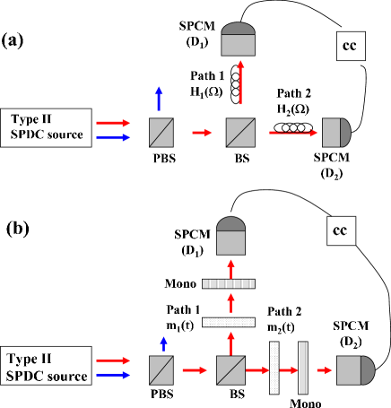
Figure 2: (Color online) General configurations for observing intrabeam correlations in (a) the temporal domain and (b) the frequency domain. PBS: Polarizing beam splitter; BS: Beam Splitter; SPCM: Single photon counting module; cc: coincidence counting; Mono: Monochromator. In (a) there are two single-mode fibers in paths $1$ and $2$ with transfer functions $H_{1}(\Omega)$ and $H_{2}(\Omega)$, respectively. In (b), there are two temporal phase modulators with transfer functions $m_{1}(t)$ and $m_{2}(t)$. Red and blue lines describe photons with orthogonal polarizations. Photons with a given polarization are discarded.

IV.1 Remote dispersion compensation in the intrabeam configuration

Let us consider the situation depicted in Fig. 2(a). After traversing the dispersive media located in paths $1$ and $2$, the probability to detect a photon in path $1$ at time $t$ in coincidence with a photon in path $2$ at time $t+\tau$ is given by the intrabeam second-order correlation function,

$$G^{(2)}_{\textrm{intra}}(\tau)=\langle a^{\dagger}_{s1}(t)a^{\dagger}_{s2}(t+\tau)a_{s2}(t+\tau)a_{s1}(t)\rangle.$$ (17)

By analogy to the case of the previous section, the corresponding operators are calculated as $a_{s(1,2)}(t)=\int\textrm{d}\Omega\tilde{a}_{s}(\Omega)H_{1(2)}(\Omega)\exp(-i\Omega t)$, where $H_{1(2)}(\Omega)$ denotes the complex transfer function placed in the path of photon 1(2). Substituting these expressions and taking into account Eqs. (5) and (6), it is easy to show that

$$G_{\textrm{intra}}^{(2)}(\tau)=N^{2}+\frac{1}{(2\pi)^{2}}\left|\int\textrm{d}\Omega\,S(\Omega)\right.$$

$$\left.\times H_{1}^{*}(\omega_{0}+\Omega)H_{2}(\omega_{0}+\Omega)\exp\left(i\Omega\tau\right)\right|^{2},$$ (18)

where $S(\Omega)=|V(\Omega)|^{2}$. We observe that the joint probability detection contains the same background term as in the interbeam case. Even more, the functional dependence on $\tau$ depends on the multiplication of the transfer functions of the dispersive media in such a way, that their phase difference may alter completely the output. However, now the previous role of the spectrum $R(\Omega)=U(\Omega)V(-\Omega)$ is replaced by the signal’s photon spectrum $S(\Omega)$.

For the sake of comparison, we derive the expression of $G^{(2)}_{\textrm{intra}}(\tau)$ in the absence of dispersive media:

$$G_{\textrm{intra}}^{(2)}(\tau)=N^{2}+\left|\Gamma(\tau)\right|^{2},$$ (19)

where $\Gamma(\tau)=1/(2\pi)\,\int\textrm{d}\Omega\exp(i\Omega\tau)S(\Omega)$. Notice that a similar suppression of the effects of dispersion can be obtained if both dispersive media are identical, i.e., $H_{1}\equiv H_{2}$. In contrast to the interbeam case, the suppression of the dispersive effects is not limited to even-order dispersion terms, but it affects all the terms victor2009 . On the other hand, the signal-to-background ratio is maximally bounded to $2$, thus challenging the observation of the effect in an experiment. The factor of $2$ is a manifestation of the thermal-like character of the intrabeam correlations. Note that a reduced signal-to-background ratio could also be attained in the interbeam correlations provided that sufficient multiple pairs were generated in the SPDC process.

IV.2 Remote temporal modulation compensation in the intrabeam configuration

Finally, we revisit the temporal modulation cancelation scheme with the photons from only one of the downconverted beams (signal, for example), as depicted in Fig. 2(b). After modulation, the probability to detect a photon in path $1$ with frequency $\omega_{0}+\Omega_{1}$ in coincidence with a photon in path $2$ with frequency $\omega_{0}+\Omega_{2}$ is provided by the magnitude

$$\tilde{G}^{(2)}_{\textrm{intra}}(\Omega_{1},\Omega_{2})=\langle\tilde{a}_{s1}^{\dagger}(\Omega_{1})\tilde{a}_{s2}^{\dagger}(\Omega_{2})\tilde{a}_{s2}(\Omega_{2})\tilde{a}_{s1}(\Omega_{1})\rangle.$$ (20)

To calculate the evolution of the operators, one just has to proceed as in section III(B), i.e., to calculate the convolution of the signal operator with the modulator transfer function in the spectral domain. Then

$$\tilde{G}_{\textrm{intra}}^{(2)}(\Omega_{1},\Omega_{2}) = N_{s}(\Omega_{1})N_{s}(\Omega_{2})$$ (21)

$$+\left|T^{\prime}(\Omega_{1},\Omega_{2})\right|^{2},$$

where

$$T^{\prime}(\Omega_{1},\Omega_{2})=\frac{1}{2\pi}\int\textrm{d}\Omega^{\prime}S(\Omega^{\prime})$$

$$\times M_{1}^{*}(\Omega_{1}-\Omega^{\prime})M_{2}(\Omega_{2}-\Omega^{\prime}).$$ (22)

As before, we obtain a background term proportional to the number of photons in modes $\omega_{0}+\Omega_{1}$ and $\omega_{0}+\Omega_{2}$. The second term is a non-separable function in frequency which is affected by the transfer functions of the modulators. Analogously to the derivation of Eq. (III.2), we can consider low-bandwidth modulators, so that this function reduces to

$$T^{\prime}(\Omega_{1},\Omega_{2})=S(\Omega_{+}/2)$$

$$\times\sum_{n=-\infty}^{\infty}J_{n}(\Delta\theta_{1}-\Delta\theta_{2})\delta(\Omega_{-}-n\Omega_{m}).$$ (23)

To close the loop, we calculate the second-order correlation function that would be achieved in the absence of modulators,

$$\tilde{G}_{\textrm{intra}}^{(2)}(\Omega_{1},\Omega_{2})=N_{s}(\Omega_{1})N_{s}(\Omega_{2})+$$

$$\left|S(\Omega_{1})\right|^{2}\delta(\Omega_{1}-\Omega_{2}).$$ (24)

Similarly to the interbeam case, there is a strong correlation between photons in paths $1$ and $2$ with the same frequency. Giving a further step, from Eq. (IV.2), if $\Delta\theta_{1}=\Delta\theta_{2}$, i.e., photons in paths $1$ and $2$ are equally phase modulated, the effects of the temporal phase modulation are suppressed. Now, the only non-zero term is $n=0$, and therefore only the detection of photons with frequencies $\Omega_{1}=\Omega_{2}$ is enhanced.

The origin of these suppression (cancelation) effects when the photons that follow paths $1$ and $2$ are equally phase-modulated, or traverse equal dispersive media, is the existence of frequency correlation between the signal photons, i.e., $\langle\tilde{a}_{s}^{\dagger}(\Omega_{1})\tilde{a}_{s}(\Omega_{2})\rangle=S(\Omega_{2})\delta(\Omega_{2}-\Omega_{1})$. Eqs. (IV.1) and (IV.2), which allow for the remote dispersion and temporal modulation cancelation, make an explicit use of the existence of these characteristic frequency correlations. This strong frequency correlation could be revealed measuring, before any temporal phase modulation takes place, the number of photons in path $1$ with frequency $\omega_{0}+\Omega_{1}$ in coincidence with the signal photons with frequency $\omega_{0}+\Omega_{2}$ that traverse path $2$, which is given by Eq. (IV.2).

V Summary and conclusions

We have considered the effects of cancelation of dispersion and temporal modulation in the regime of multiphoton pair generation in the SPDC process. The two schemes are studied with two kinds of photon correlations, those arising from the downconverted signal and idler photons (interbeam correlations), which show entanglement, and those from the individual photons in a single beam (intrabeam correlations), which show strong correlations but not entanglement. In the intrabeam regime, it is possible to achieve the suppression of the effects of either dispersion or temporal modulation at all orders.

An important point to remark is that the observation of the remote cancelation of the dispersion and modulation effects in the interbeam configuration happens even in the high-flux regime ($\sigma L\gg 1$). In this case, an inequality of normalized second-order correlation functions howell2006 ; mancini2002 which is fulfilled by classical-like fields, is no longer violated. This highlights the role of the frequency anticorrelation and correlation effects as the reason for the observation of any dispersion or modulation cancelation effects.

The observation in a particular setting of dispersion and modulation cancelation effects depends on the type of frequency correlations present. In the interbeam case, where the photons show frequency anticorrelation, the observation of dispersion and modulation cancelation effects requires that both photons suffer only even-order dispersion of the opposite sign, or identical phase modulation but with opposite phases.

On the other hand, if the photons are frequency correlated (intrabeam correlations with $\Omega_{1}-\Omega_{2}=0$), the observation of dispersion and modulation cancelation effects requires that both photons suffer equal dispersion, for all dispersion terms, or identical phase modulation, with the same phases.

The effects described here bear important similarities with the description of two-photon imaging experiments with two different types of two-photon sources: paired photons entangled in the spatial degree of freedom and bunched pairs of photons coming from a thermal light source scarcelli2004 . In pittman1995 , a two-photon optical imaging experiment was performed based on the spatial correlations of the signal and idler photon pairs produced in SPDC. The possibility to use thermal (or pseudothermal) radiation for two-photon imaging experiments has also been demonstrated valencia2005 . In both cases, the important point that enables the observation of similar effects with dissimilar sources is the presence of spatial correlations between the paired photons.

Again, the spatial correlations between signal and idler photons show different characteristics than the spatial correlations of signal pairs. But the observation of two-photon imaging, as well as the capacity to cancel diffraction effects when measuring two-photon coincidences, are due to some of the common characteristics that both types of sources share: the presence of certain correlations between paired photons.

References

- (1) R. J. Glauber, Phys. Rev. 131, 2766 (1963).
- (2) R. J. Glauber, Rev. Mod. Phys. 78, 1267 (2006).
- (3) L. Mandel and E. Wolf, Optical coherence and quantum optics, Cambridge University Press, 1995.
- (4) A. Kuzmich, W. P. Bowen, A. D. Boozer, A. Boca, C. W. Chou, L.-M. Duan, H. J. Kimble, Nature 423, 731 (2003).
- (5) R. Loudon, Quantum Theory of Light, Oxford University Press, 1st edition 1973, 3rd edition 2000.
- (6) J. D. Franson, Phys. Rev. A 45, 3126 (1992).
- (7) J. Brendel, H. Zbinden and N. Gisin, Opt. Comm. 151, 35 (1998).
- (8) S. Y. Baek, Y. W. Cho and Y. H. Kim, Opt. Express 17, 19244 (2009).
- (9) A. Valencia, M. V. Chekhova, A. Trifonov and Y. Shih, Phys. Rev. Lett. 88, 183601 (2002).
- (10) S. E. Harris, Phys. Rev. A 78, 021807 (2008).
- (11) S. Sensarn, G. Y. Yin, and S. E. Harris, Phys. Rev. Lett. 103, 163601 (2009).
- (12) V. Torres-Company, H. Lajunen, and A. T. Friberg, New J. Phys. 11, 063041 (2009).
- (13) J. H. Shapiro, Phys. Rev. A 81 023824 (2010).
- (14) J. D. Franson, Phys. Rev. A 80, 032119 (2009).
- (15) J. D. Franson, Phys. Rev. A 81, 023825 (2010).
- (16) B. Dayan, Phys. Rev. A 76, 043813 (2007).
- (17) P. Navez, E. Brambilla, A. Gatti, and L. A. Lugiato, Phys. Rev. A 65, 013813 (2001).
- (18) E. Brambilla, A. Gatti, M. Bache, and L. A. Lugiato, Phys. Rev. A 69, 023802 (2004).
- (19) B. Blauensteiner, I. Herbauts, S. Bettelli, A. Poppe, and H. Hübel, Phys. Rev. A 79, 063846 (2009).
- (20) B. Yurke and M. Potasek, Phys. Rev. A 36, 3464 (1987).
- (21) V. Balic, D. A. Braje, P. Kolchin, G. Y. Yin, and S. E. Harris, Phys. Rev. Lett. 94, 183601 (2005).
- (22) I. A. Khan and J. C. Howell, Phys. Rev. A 73, 031801(R) (2006).
- (23) S. Mancini, V. Giovannetti, D. Vitali, and P. Tombesi, Phys. Rev. Lett. 88, 120401 (2002).
- (24) G. Scarcelli, A. Valencia, and Y. Shih, Phys. Rev. A 70 051802 (2004).
- (25) T. B. Pittman, Y. Shih, D. V. Strekalov, and A. V. Sergienko, Phys. Rev. A, 52, 3429(R) (1995).
- (26) A. Valencia, G. Scarcelli, M. D Angelo, and Y. Shih, Phys. Rev. Lett. 94 063601 (2005).