Complexified Cones.
Spectral gaps and variational principles.

Abstract

We consider contractions of complexified real cones, as recently introduced by Rugh in [Rugh10]. Dubois [Dub09] gave optimal conditions to determine if a matrix contracts a canonical complex cone. First we generalize his results to the case of complex operators on a Banach space and give precise conditions for the contraction and an improved estimate of the size of the associated spectral gap. We then prove a variational formula for the leading eigenvalue similar to the Collatz-Wielandt formula for a real cone contraction. Morally, both cases boil down to the study of suitable collections of 2 by 2 matrices and their contraction properties on the Riemann sphere.

1 Introduction

The notion of a complex cone contraction with an associated hyperbolic projective metric was introduced by Rugh in [Rugh10]. There, it was shown that a complex operator has a ‘spectral gap’ if it contracts a suitable complex cone. In this context we say that a bounded linear operator $A\in L(X)$ on a complex Banach space has a spectral gap if it has a non-zero eigenvalue $\lambda$ and an associated one dimensional projection $P$ so that $AP=PA=\lambda P$ and $A-\lambda P$ has a spectral radius strictly smaller than $|\lambda|$. The quantity $\eta_{\rm sp}(A)=r_{\rm sp}(A-\lambda P)/|\lambda|<1$ is a measure of the size of this gap.

A simpler hyperbolic metric was subsequently introduced by Dubois in [Dub09], who gave explicit estimates for the size of the spectral gap in the case of matrices. We show here that his simple estimate carries over to a linear operator that contracts a complexified real cone in any complexified Banach space.

We also consider the problem of giving lower bounds for the leading eigenvalue. This was left as an open problem in [Rugh10, Remark 3.8]. Our key observation is that we may associate to any complexified real cone a natural pre-order. Using this we show that the leading eigenvalue is given by a variational or max/min principle. This generalizes the well-known Collatz-Wielandt formula for a real cone contraction (see [C42, W50] and e.g. [M88, Section 1.3] for a more modern treatment).

We present here only results for complexified real cones as they are computationally much simpler to treat than general complex cones. The upshot both for the spectral gap and the lower bound is that it suffices to look at certain collections of complex 2 by 2 matrices of ‘matrix elements’ and the contraction properties of the associated linear fractional transformations on the Riemann sphere. For our proofs we rely upon [Dub09] for matricial calculations and [Rugh10] for the spectral gap properties.

2 Assumptions and results

Let $X_{{\mathbb{R}}}$ be a real Banach space and $X$ a complexification of $X_{{\mathbb{R}}}$. $X^{\prime}_{{\mathbb{R}}}$ and $X^{\prime}$ signify the corresponding dual spaces and we write $\langle\cdot,\cdot\rangle:X^{\prime}_{{\mathbb{R}}}\times X_{{\mathbb{R}}}\rightarrow{{\mathbb{R}}}$ and $\langle\cdot,\cdot\rangle:X^{\prime}\times X\rightarrow{\mathbb{C}}$ for the canonical dualities. Let ${K}_{{{\mathbb{R}}}}$ be a real, convex, closed and proper cone (we call it an ${{\mathbb{R}}}$-cone) in $X_{{\mathbb{R}}}$, i.e. ${K}_{{{\mathbb{R}}}}$ is closed and verifies ${K}_{{{\mathbb{R}}}}+{K}_{{{\mathbb{R}}}}={K}_{{{\mathbb{R}}}}$, ${{\mathbb{R}}}_{+}{K}_{{{\mathbb{R}}}}={K}_{{{\mathbb{R}}}}$ and ${K}_{{{\mathbb{R}}}}\cap-{K}_{{{\mathbb{R}}}}=\{0\}$. Denote by ${{K}^{\;{}^{\prime}}_{{{\mathbb{R}}}}}=\{\ell\in X^{\prime}:\langle\ell,x\rangle\geq 0,\ \ \forall x\in{K}_{{{\mathbb{R}}}}\}$ the dual cone of ${K}_{{{\mathbb{R}}}}$. It is itself convex and closed. By a separation theorem the cone itself is recovered from ${K}_{{{\mathbb{R}}}}=\{x\in X:\langle\ell,x\rangle\geq 0,\ \ \forall\,\ell\in{{K}^{\;{}^{\prime}}_{{{\mathbb{R}}}}}\}$.

Following [Rugh10] we define the canonical complexification of the real cone:

$${{{K}}_{{\mathbb{C}}}}=\left\{{\rule[-4.30554pt]{0.0pt}{9.47217pt}{}}x\in X:{\rm Re\,}\langle\ell_{1},x\rangle\overline{\langle\ell_{2},x\rangle}\geq 0,\ \ell_{1},\ell_{2}\in{{K}^{\;{}^{\prime}}_{{{\mathbb{R}}}}}\right\}$$ (2.1)

We also denote by

$${{{K}}^{\;{}^{\prime}}_{{\mathbb{C}}}}=\left\{{\rule[-4.30554pt]{0.0pt}{9.47217pt}{}}\mu\in X^{\prime}:{\rm Re\,}\langle\mu,x_{1}\rangle\overline{\langle\mu,x_{2}\rangle}\geq 0,\ x_{1},x_{2}\in{K}_{{{\mathbb{R}}}}\right\}.$$ (2.2)

the complexified dual cone (note that this is somewhat different from the ‘dual cone’ of Definition 2.3 in [Dub09]). We use a ‘star’ to denote the omission of the zero-vector, e.g. ${({{K}}_{{\mathbb{C}}})^{*}}={{{K}}_{{\mathbb{C}}}}\setminus\{0\}$.

Definition 2.1

We define a pre-order of non-zero elements $x,y\in{({{K}}_{{\mathbb{C}}})^{*}}$:

$$x\succeq y\ \ \ \ \mbox{iff}\ \ \ \ \forall\mu\in{{{K}}^{\;{}^{\prime}}_{{\mathbb{C}}}}:|\langle\mu,x\rangle|\geq|\langle\mu,y\rangle|.$$ (2.3)

Adapting the conventions  $\inf\emptyset=+\infty$  and  $\sup\emptyset=0$  we set:

$$\alpha(x,y)=\sup\{t\geq 0:x\succeq ty\}\ \ \ \ \mbox{and}\ \ \ \ \beta(x,y)=\inf\{t\geq 0:x\preceq ty\}.$$ (2.4)

One has $\alpha(x,y)=1/\beta(y,x)\in[0,+\infty)$. By Lemma 8.1 below, ${{{K}}^{\;{}^{\prime}}_{{\mathbb{C}}}}$ separates points in ${{{K}}_{{\mathbb{C}}}}$ so there is always $\mu\in{{{K}}^{\;{}^{\prime}}_{{\mathbb{C}}}}$ for which $\langle\mu,y\rangle\neq 0$. We therefore have the equivalent expression:

$$\beta(x,y)=\sup\left\{\left|\frac{\langle\mu,x\rangle}{\langle\mu,y\rangle}\right|\ :\ \mu\in{{{K}}^{\;{}^{\prime}}_{{\mathbb{C}}}},\left(\!\begin{array}[]{c}\langle\mu,x\rangle\\ \langle\mu,y\rangle\end{array}\!\right)\neq\left(\!\begin{array}[]{c}0\\ 0\end{array}\!\right)\right\}.$$ (2.5)

• It is possible to give an intrinsic definition of our pre-order not involving any dual cone. For $x,y\in{({{K}}_{{\mathbb{C}}})^{*}}$, we have (see Proposition B.1)

  $$x\succeq y\ \ \ \ \mbox{iff}\ \ \ \ \forall\alpha\in\mathbb{C},|\alpha|<1:x-\alpha y\in{({{K}}_{{\mathbb{C}}})^{*}}.$$ (2.6)

  An important feature of complexified cones is that the right hand side of the preceding equation actually defines a transitive relation.

Proposition 2.2

For $x,y\in{({{K}}_{{\mathbb{C}}})^{*}}$ let

$$d_{{{{K}}_{{\mathbb{C}}}}}(x,y)\ =\ \log\left(\,\beta(x,y)\;\beta(y,x)\,\right)=\log\left(\frac{\beta(x,y)}{\alpha(x,y)}\right)\ \ \in\ \ [0,+\infty].$$ (2.7)

Then $d_{{{K}}_{{\mathbb{C}}}}$ defines a projective (pseudo-)metric on ${({{K}}_{{\mathbb{C}}})^{*}}$ for which $d_{{{K}}_{{\mathbb{C}}}}(x,y)=0$ iff $x$ and $y$ belong to the same complex line. The map $x,y\in{({{K}}_{{\mathbb{C}}})^{*}}\mapsto d_{{{{K}}_{{\mathbb{C}}}}}(x,y)\in[0,+\infty]$ is lower semi-continuous.

Given a subset $S$ of a real or complex vector space we write $\,{{\mathbb{R}}}_{+}\,(S)=\{\sum_{\rm finite}t_{k}u_{k}:t_{k}\geq 0,u_{k}\in S\}$ for the real cone generated by this set. We will need some further assumptions relating the cones to generating sets and to the topology of the Banach space:

Definition 2.3

1. A subset $S$ of a real or complex vector space is said to be a generating set for a closed cone $K$ if $S$ does not contain the zero-vector and $K={\rm Cl\;}\,{{\mathbb{R}}}_{+}\,(S)$.

2. When ${\cal E}$ is a generating set for ${K}_{{{\mathbb{R}}}}$ we say that ${\cal E}$ is Archimedian if for every $x\in{K}_{{{\mathbb{R}}}}^{*}$ there exists $e\in{\cal E}$ and $t>0$ so that $x-te\in{K}_{{{\mathbb{R}}}}$.

3. We say that ${K}_{{{\mathbb{R}}}}$ is of $\kappa$-bounded sectional aperture (for some $\kappa>0$) provided that for any two dimensional plane $V=V(x,y)={\rm Span}\{x,y\}$ we may find a real linear functional $m$ of norm one for which: $\|\xi\|\leq\kappa\langle m,\xi\rangle$ for all $\xi\in{K}_{{{\mathbb{R}}}}\cap V$.

4. We say that ${K}_{{{\mathbb{R}}}}$ is reproducing if there is $g<+\infty$ so that for every $x\in X_{{\mathbb{R}}}$ we may find $y_{1},y_{2}\in{K}_{{{\mathbb{R}}}}$, with $x=y_{1}-y_{2}$ and $\|y_{1}\|+\|y_{2}\|\leq g\|x\|$.

One could, of course, take the real cone (and its dual) themselves as generating sets, but many interesting situations occur where it is natural to consider smaller generating sets. The simplest example is the canonical basis in ${{\mathbb{R}}}^{n}$ which generates the standard positive cone ${{\rule[0.0pt]{0.0pt}{8.61108pt}{}}\mathbb{R}}{\rule[0.0pt]{0.0pt}{8.61108pt}{}}_{+}^{\hskip 0.45206ptn}$. When ${K}_{{{\mathbb{R}}}}$ is finitely generated by ${\cal E}$ then ${K}_{{{\mathbb{R}}}}$ is per se Archimedian but in general this need not be true. Already for a real cone contraction one needs something like the Archimedian propery in order to get a spectral gap:

Example 2.4

Consider $X=L^{2}([0,1])$ and ${K}_{{{\mathbb{R}}}}=\{f\in X:f\geq 0\ \ (a.s)\}$. One verifies that the set ${\cal E}=\{{\bf 1}_{[a,b]}:0\leq a<b\leq 1\}$ of indicator functions on intervals generates ${K}_{{{\mathbb{R}}}}$ but is not Archimedian. For example, if $A\subset[0,1]$ is compact, without interior but of positive Lebesgue measure (a fat Cantor set) then ${\bf 1}_{A}$ is not greater than  $te$   for any $t>0$ and $e\in{\cal E}$. The operator $Tf={\bf 1}_{A}\cdot\int f(1-{\bf 1}_{A})$ maps ${K}_{{{\mathbb{R}}}}$ to ${K}_{{{\mathbb{R}}}}$, is strictly positive on ${\cal E}$ and is a strict contraction (the image is in fact one dimensional) but $T^{2}\equiv 0$ so it has no spectral gap. We want to avoid this situation. When ${\cal E}$ is an Archimedian generating set for ${K}_{{{\mathbb{R}}}}$ and $A({\cal E})\subset{K}_{{{\mathbb{R}}}}^{*}$ then it is easy to see that if $x\in{K}_{{{\mathbb{R}}}}^{*}$ (so is non-zero), then also $Ax\in{K}_{{{\mathbb{R}}}}^{*}$. Below we show that a similar property holds in the complex setting.

Assumption 2.5

In the sequel we will make the following standing assumptions: Let $A\in L(X_{1};X_{2})$ be a bounded linear (complex) operator between two complex Banach spaces $X_{1}$ and $X_{2}$. Each Banach space is assumed to be a complexification of a real Banach space ${{X}_{{{\mathbb{R}}},1}}$ and ${{X}_{{{\mathbb{R}}},2}}$ and to come with proper closed convex cones ${{{K}}_{{{\mathbb{R}}},1}}\subset{{X}_{{{\mathbb{R}}},1}}$ and ${{{K}}_{{{\mathbb{R}}},2}}\subset{{X}_{{{\mathbb{R}}},1}}$, respectively. We denote by ${{{K}}_{{\mathbb{C}},1}}\subset X_{1}$ and ${{{K}}_{{\mathbb{C}},2}}\subset X_{2}$ the respective canonical complexified cones. We suppose that ${\cal E}_{1}$ is a generating set for ${{{K}}_{{{\mathbb{R}}},1}}$ and that ${\cal M}_{2}$ is a weak-$*$ generating set for ${{{K}}^{\;{}^{\prime}}_{{{\mathbb{R}}},2}}$. Thus, ${\cal E}_{1}\subset({{{K}}_{{{\mathbb{R}}},1}})^{*}$ and ${\rm Cl\;}\,{{\mathbb{R}}}_{+}\,({\cal E}_{1})={{{K}}_{{{\mathbb{R}}},1}}$ and when $\mu\in{{{K}}^{\;{}^{\prime}}_{{{\mathbb{R}}},2}}$ then for any choice of $y_{1},\dots,y_{p}\in X_{2}$, $\epsilon>0$ we may find $\ell\in\,{{\mathbb{R}}}_{+}\,({\cal M}_{2})$ for which $\left|\langle\ell,y_{k}\rangle-\langle\mu,y_{k}\rangle\right|<\epsilon$, $k=1,\ldots,p$. When $X_{1}=X_{2}$ and the cones are identical we will simply omit the indices in our notation.

Our treatment relies upon a close study of the contraction properties of complex 2 by 2 matrices. Two classes of such matrices are of particular interest in our context:

$$\overset{\circ}{\Gamma}{\rule[0.0pt]{0.0pt}{8.61108pt}{}}_{+}=\left\{\left(\!\begin{array}[]{cc}a&b\\ c&d\end{array}\!\right):{|ad-bc|}\ <\;{\rm Re\,}(a\overline{\rule[0.0pt]{0.0pt}{8.94441pt}{}{d}}+b\overline{\rule[0.0pt]{0.0pt}{6.30551pt}{}{c}}),\ \ \ {\rm Re\,}a\,\overline{\rule[0.0pt]{0.0pt}{8.94441pt}{}{b}},\ a\,\overline{\rule[0.0pt]{0.0pt}{6.30551pt}{}{c}},\ b\,\overline{\rule[0.0pt]{0.0pt}{8.94441pt}{}{d}},\ c\,\overline{\rule[0.0pt]{0.0pt}{8.94441pt}{}{d}}\;>0\right\}.\ \$$ (2.8)

$$\overline{{\rule[0.0pt]{0.0pt}{8.61108pt}{}}\Gamma}{\rule[0.0pt]{0.0pt}{8.61108pt}{}}_{+}=\left\{\left(\!\begin{array}[]{cc}a&b\\ c&d\end{array}\!\right):|ad-bc|\ \leq\;{\rm Re\,}(a\overline{\rule[0.0pt]{0.0pt}{8.94441pt}{}{d}}+b\overline{\rule[0.0pt]{0.0pt}{6.30551pt}{}{c}}),\ \ \ {\rm Re\,}a\,\overline{\rule[0.0pt]{0.0pt}{8.94441pt}{}{b}},\ a\,\overline{\rule[0.0pt]{0.0pt}{6.30551pt}{}{c}},\ b\,\overline{\rule[0.0pt]{0.0pt}{8.94441pt}{}{d}},\ c\,\overline{\rule[0.0pt]{0.0pt}{8.94441pt}{}{d}}\;\geq 0\right\}.$$ (2.9)

A matrix $T\in\overset{\circ}{\Gamma}{\rule[0.0pt]{0.0pt}{8.61108pt}{}}_{+}$ is ‘contracting’ in the sense of Appendix A. The ‘contraction rate’ is controlled by the ratio of the LHS to the RHS in the inequality in (2.8). We may therefore define families of ‘uniformly contracting’ matrices as follows:

Definition 2.6

With $0\leq\theta<1$ as a parameter we set $\ \displaystyle{\Gamma}{\rule[0.0pt]{0.0pt}{8.61108pt}{}}_{+}\left(\theta\right)=\left\{T\in\overset{\circ}{\Gamma}{\rule[0.0pt]{0.0pt}{8.61108pt}{}}_{+}:\frac{|ad-bc|}{{\rm Re\,}(a\overline{\rule[0.0pt]{0.0pt}{8.94441pt}{}{d}}+b\overline{\rule[0.0pt]{0.0pt}{6.30551pt}{}{c}})}\leq\theta\right\}.$ We also associate to this parameter $\displaystyle\delta_{1}(\theta)\equiv\log\frac{1+\theta}{1-\theta}$ and

$$\eta_{\,1}(\theta)\equiv\tanh\frac{9\delta_{1}(\theta)}{4}=\frac{\left(1+\theta\right)^{9/2}-\left(1-\theta\right)^{9/2}}{\left(1+\theta\right)^{9/2}+\left(1-\theta\right)^{9/2}}\ <\ 1\ .$$ (2.10)

Given couples $e_{1},e_{2}\in{\cal E}_{1}$ and $m_{1},m_{2}\in{\cal M}_{2}$ we define the complex 2 by 2 matrix:

$$T=T(m_{1},m_{2};Ae_{1},Ae_{2})\equiv\left(\!\begin{array}[]{cc}\langle m_{1},Ae_{1}\rangle&\langle m_{2},Ae_{1}\rangle\\ \langle m_{1},Ae_{2}\rangle&\langle m_{2},Ae_{2}\rangle\end{array}\!\right)$$ (2.11)

We write ${\cal T}(A)\subset M_{2}({\mathbb{C}})$ for the collection of such 2 by 2 matrices. Our first theorem gives a characterization of a complexified cone contraction. With $A$ and ${\cal T}(A)$ as above we have the following:

Theorem 2.7

${\cal T}(A)\subset\overline{{\rule[0.0pt]{0.0pt}{8.61108pt}{}}\Gamma}{\rule[0.0pt]{0.0pt}{8.61108pt}{}}_{+}$    iff   $A({{{K}}_{{\mathbb{C}},1}})\subset{{{K}}_{{\mathbb{C}},2}}$   and   $A^{\prime}({{{K}}^{\;{}^{\prime}}_{{\mathbb{C}},2}})\subset{{{K}}^{\;{}^{\prime}}_{{\mathbb{C}},1}}$.

Remark 2.8

There is also ‘almost’ an equivalence between  $A({{{K}}_{{\mathbb{C}},1}})\subset{{{K}}_{{\mathbb{C}},2}}$  and  $A^{\prime}({{{K}}^{\;{}^{\prime}}_{{\mathbb{C}},2}})\subset{{{K}}^{\;{}^{\prime}}_{{\mathbb{C}},1}}$. The only (pathological) exception is when the rank of $A$ is one in which case this equivalence may fail. We do not need this and omit the proof.

Let $d_{1}=d_{{{{K}}_{{\mathbb{C}},1}}}$ and $d_{2}=d_{{{{K}}_{{\mathbb{C}},2}}}$ be the projective metrics associated to $({{{K}}_{{\mathbb{C}},1}})^{*}$ and $({{{K}}_{{\mathbb{C}},2}})^{*}$, respectively (as in Proposition 2.2). Our second Theorem states that knowing that the family ${\cal T}(A)$ is uniformly contracting suffices to conclude that we are dealing with a projective cone-contraction and furthermore to give a bound for the contraction rate:

Theorem 2.9

Let $A$, ${\cal E}_{1}$, ${\cal M}_{2}$, ${\cal T}(A)$ be as above. Suppose that ${\cal E}_{1}$ is Archimedian and that ${\cal T}(A)\subset{\Gamma}{\rule[0.0pt]{0.0pt}{8.61108pt}{}}_{+}\left(\theta\right)$ for some $\theta\in[0,1)$. Then $A$ maps $({{{K}}_{{\mathbb{C}},1}})^{*}$ into $({{{K}}_{{\mathbb{C}},2}})^{*}$ and the mapping $A:(({{{K}}_{{\mathbb{C}},1}})^{*},d_{1})\rightarrow(({{{K}}_{{\mathbb{C}},2}})^{*},d_{2})$ is $\eta_{\,1}(\theta)$-Lipschitz.

Considering the situation when $X=X_{1}=X_{2}$ and the cones in the two spaces are the same (so we omit indices in the notation) we obtain:

Theorem 2.10

Let $A\in L(X)$, ${\cal E}$, ${\cal M}$, ${\cal T}(A)$ be as above with ${\cal E}$ Archimedian. We assume that ${K}_{{{\mathbb{R}}}}$ is of $\kappa$-bounded sectional aperture and is reproducing. If ${\cal T}(A)\subset{\Gamma}{\rule[0.0pt]{0.0pt}{8.61108pt}{}}_{+}\left(\theta\right)$ for some $\theta\in[0,1)$ then $A$ has a spectral gap for which $\eta_{\rm\;sp}\;(A)\leq\eta_{\,1}(\theta)<1$. More precisely, there are elements $h\in{{{K}}_{{\mathbb{C}}}}$, $\nu\in{{{K}}^{\;{}^{\prime}}_{{\mathbb{C}}}}$, and constants $\lambda\in{\mathbb{C}}^{*}$, $C<+\infty$ so that for all $n\geq 1$ and $x\in X$:

$$\|\lambda^{-n}A^{n}x-h\langle\nu,x\rangle\|\leq C\;\left(\eta_{\,1}(\theta)\right)^{n-1}\;\|x\|.$$ (2.12)

Moreover, for every $x\in{({{K}}_{{\mathbb{C}}})^{*}}$ we have $\langle\nu,x\rangle\neq 0$.

The spectral gap has its origin in the Lipschitz contraction rate so we get also for free the following sub-multiplicative property:

Corollary 2.11

If $(A_{n})_{n\geq 1}$ is a sequence of operators satifying the hypotheses of Theorem 2.10 with each ${\cal T}(A_{n})\subset{{\rule[0.0pt]{0.0pt}{8.61108pt}{}}\Gamma}{\rule[0.0pt]{0.0pt}{8.61108pt}{}}_{+}(\theta_{n})$, $\theta_{n}<1$. Then for any $n\geq 1$, the product $A_{1}\cdots A_{n}$ (in general non-commuting) has a a spectral gap which verifies the inequality

$$\eta_{\rm\;sp}\;(A_{1}\ldots A_{n})\leq\eta_{\,1}(\theta_{1})\ldots\eta_{\,1}(\theta_{n})<1.$$

Remarks 2.12

1. In the proofs of Theorems 2.9 and 2.10 we actually obtain a better bound for the contraction rate. The Lipschitz contraction take place at a rate which is bounded by

   $$\tanh\left(\Delta_{1}(A)+\frac{1}{2}\Delta_{2}(A)+\frac{1}{2}\Delta_{3}(A)+\frac{1}{4}\Delta_{4}(A)\right)$$ (2.13)

   where $\Delta_{i}(A)=\sup_{T\in{\cal T}(A)}\Delta_{i}(T^{t})\;\in\;[0,+\infty]$ and $\Delta_{i}(T)$ is defined in Appendix A. The contraction numbers are ordered as follows: $0\leq\Delta_{4}(A)\leq\Delta_{2,3}(A)\leq\Delta_{1}(A)\leq\delta_{1}(\theta)$, so the RHS in (2.13) is bounded by the simpler expression $\eta_{1}(\theta)=\tanh\frac{9\delta_{1}(\theta)}{4}$ as stated in the Theorems.

2. It is not clear if the factor 9 (appearing in e.g. (2.10)) is optimal (for the bounds in e.g. Theorem 2.10 to hold). It comes for complex reasons. For a real operator acting on real cones it is unity. But in the general case it can not be smaller than 3 (we omit the proof).

3. In [Dub09, Theorem 3.7], for the case of matrices, an apparently weaker result for the contraction factor was published. But as noted in [Dub09-2] this actually reduces to the factor in our Theorem 2.10.

3 Integral operators and spectral gaps

Let $(\Omega,\mu)$ be a $\sigma$-finite measure space and let $X=L^{p}(\Omega,\mu)$ for $1\leq p\leq+\infty$. We denote by $q=p/(p-1)\in[1,+\infty]$ the conjugate exponent. Suppose that $k:\Omega\times\Omega\rightarrow{\mathbb{C}}$ is measurable and that there is $C<+\infty$ such that for every $\ g\in L^{p}(\Omega,\mu),f\in L^{q}(\Omega,\mu)$:

$$\int_{\Omega}\int_{\Omega}|f(x)k(x,y)g(y)|d\mu(x)d\mu(y)\leq C\|f\|_{L^{q}}\|g\|_{L^{p}}.$$ (3.14)

Then $k$ is the integral kernel for a bounded linear operator ${\cal L}:L^{p}(\Omega,\mu)\rightarrow L^{p}(\Omega,\mu)$ given by

$$({\cal L}\phi)(y)=\int_{\Omega}k(x,y)\phi(y)d\mu(x).$$ (3.15)

Our goal hear is to give sufficient conditions for ${\cal L}$ to have a spectral gap and to give an estimate for the size of the gap. For $x_{1},x_{2},y_{1},y_{2}\in\Omega$ we denote

$$N_{x_{1},x_{2};y_{1},y_{2}}=\left(\!\begin{array}[]{cc}k(x_{1},y_{1})&k(x_{1},y_{2})\\ k(x_{1},y_{2})&k(x_{2},y_{2})\end{array}\!\right).$$ (3.16)

Theorem 3.1

Suppose that for $\mu$-a.e. $x_{1},x_{2},y_{1},y_{2}\in\Omega$: $N_{x_{1},x_{2};y_{1},y_{2}}\in{\Gamma}{\rule[0.0pt]{0.0pt}{8.61108pt}{}}_{+}\left(\theta\right)$ for some $\theta\in[0,1)$. Then ${\cal L}$ has a spectral gap for which $\eta_{\rm\;sp}\;({\cal L})\leq\eta_{\,1}(\theta)<1$. We refer to (2.6) and (2.10) for the precise definitions.

Remark 3.2

Note that the above result is independent of $p\in[1,+\infty]$. In particular, it is valid also in the case $p=\infty$ where the dual of $X=L^{\infty}(\Omega,\mu)$ may be strictly larger than $L^{1}(\Omega,\mu)$.

4 Variational principles

A proper convex real cone induces a natural partial order on the Banach space:   $x\leq y$ iff $y-x\in{K}_{{{\mathbb{R}}}}$. This leads to a max-min or variational principle, the so-called Collatz-Wielandt formula, for the leading eigenvalue of a real cone contraction. In the case of a strictly positive $n$ by $n$ matrix $A$ one has for example:

$$r_{\rm sp}(A)=\max_{x\in({{\mathbb{R}}}^{n}_{+})^{*}}\ \ \inf_{1\leq i\leq n}\ \frac{(Ax)_{i}}{x_{i}}=\min_{x\in({{\mathbb{R}}}^{n}_{+})^{*}}\ \sup_{1\leq i\leq n}\ \ \frac{(Ax)_{i}}{x_{i}}$$ (4.17)

with the understanding that $k/0=+\infty$ for $k>0$ (the numerator never vanishes). Taking the transpose of $A$ one obtains two more expressions for the spectral radius.

Similar results hold for more general real cone contraction but we leave this aside as we want to look at complex cone contractions. We consider again the case of a complexified real cone and when the source and image spaces and cones are identical (so we omit indices). The pre-order in Definition 2.1 allows us to deduce a variational principle for a complex cone contraction. In the Collatz-Wielandt formula one considers ratios of non-negative real numbers. A similar construction works in the complex case but it is based upon the study of 2 by 2 complex matrices. Given $x\in{({{K}}_{{\mathbb{C}}})^{*}}$ and we consider complex 2 by 2 matrices of the form:

$$T(m_{1},m_{2};Ax,\,x)\equiv\left(\!\begin{array}[]{cc}\langle m_{1},Ax\rangle&\langle m_{2},Ax\rangle\\ \langle m_{1},x\rangle&\langle m_{2},x\rangle\end{array}\!\right),\ \ \ \ \ m_{1},m_{2}\in{\cal M}$$ (4.18)

We write ${\cal R}(A)\subset M_{2}({\mathbb{C}})$ for the collection of such matrices. The reader may notice the similarity with the set ${\cal T}(A)$ used for the contraction described previously. When $A$ is a complex cone contraction, then ${\cal R}(A)$ is a subset of the set ${\cal K}$ described in the following

Definition 4.1

Let ${\cal K}$ be the set of complex 2 by 2 matrices $M=\left(\!\begin{array}[]{cc}a&b\\ c&d\end{array}\!\right)$ for which   ${\rm Re\,}a\,\overline{\rule[0.0pt]{0.0pt}{8.94441pt}{}{b}}\,\geq\,0$  and  ${\rm Re\,}c\,\overline{\rule[0.0pt]{0.0pt}{8.94441pt}{}{d}}\,\geq\,0$. We define two maps $\Phi$ and $\phi$ from ${\cal K}$ to $[0,+\infty]$. We distinguish according to the rank of $M$. When rank $M=2$, i.e. $ad-bc\neq 0$ we set

$$\Phi(M)=\frac{|a\overline{\rule[0.0pt]{0.0pt}{8.94441pt}{}{d}}+b\overline{\rule[0.0pt]{0.0pt}{6.30551pt}{}{c}}|\;+\;|ad-bc|}{2\;{\rm Re\,}c\overline{\rule[0.0pt]{0.0pt}{8.94441pt}{}{d}}}\ \ \ \mbox{and}\ \ \ \phi(M)=\frac{2\;{\rm Re\,}a\overline{\rule[0.0pt]{0.0pt}{8.94441pt}{}{b}}}{|a\overline{\rule[0.0pt]{0.0pt}{8.94441pt}{}{d}}+b\overline{\rule[0.0pt]{0.0pt}{6.30551pt}{}{c}}|\;+\;|ad-bc|}\ .$$ (4.19)

When rank $M$=1 we set $\displaystyle\Phi(M)=\phi(M)=\left|\frac{a}{c}\right|$  $\displaystyle\left(\mbox{or}\ \left|\frac{b}{d}\right|\ \mbox{if}\ a=c=0\right)$. Finally if $M$ is identically zero, we set    $\Phi(M)=0$   and   $\phi(M)=+\infty$.

Theorem 4.2

Suppose that ${\cal T}(A)\subset\overline{{\rule[0.0pt]{0.0pt}{8.61108pt}{}}\Gamma}{\rule[0.0pt]{0.0pt}{8.61108pt}{}}_{+}$, (as in Theorem 2.7). Abbreviating   $M_{m_{1}m_{2}}=T(m_{1},m_{2};Ax,x)$   we have

$$r_{\rm sp}(A)\ \geq\ \sup_{{\rule[0.0pt]{0.0pt}{5.12358pt}{}}x\in{({{K}}_{{\mathbb{C}}})^{*}}}\ \ \alpha(Ax,x)=\sup_{{\rule[0.0pt]{0.0pt}{5.12358pt}{}}x\in{({{K}}_{{\mathbb{C}}})^{*}}}\ \ \inf_{m_{1},m_{2}\in{\cal M}}\ \phi\,(M_{m_{1}\,m_{2}}).$$ (4.20)

Theorem 4.3

Assume now the stronger contraction conditions of Theorem 2.10. Abbreviating again   $M_{m_{1}m_{2}}=T(m_{1},m_{2};Ax,x)$   we have

$$r_{\rm sp}(A) = \sup_{{\rule[0.0pt]{0.0pt}{5.12358pt}{}}x\in{({{K}}_{{\mathbb{C}}})^{*}}}\ \ \alpha(Ax,x)=\sup_{{\rule[0.0pt]{0.0pt}{5.12358pt}{}}x\in{({{K}}_{{\mathbb{C}}})^{*}}}\ \ \inf_{m_{1},m_{2}\in{\cal M}}\ \phi(M_{m_{1}m_{2}})$$ (4.21)

$$= \inf_{{\rule[0.0pt]{0.0pt}{5.12358pt}{}}x\in{({{K}}_{{\mathbb{C}}})^{*}}}\ \ \beta(Ax,x)=\inf_{x\in{({{K}}_{{\mathbb{C}}})^{*}}}\ \ \sup_{{\rule[0.0pt]{0.0pt}{5.12358pt}{}}m_{1},m_{2}\in{\cal M}}\ \Phi(M_{m_{1}m_{2}})$$ (4.22)

The extremal value is realized for the leading eigenvector $x=h\in{({{K}}_{{\mathbb{C}}})^{*}}$ (cf. Theorem 2.10).

Remark 4.4

The variational principle allows us in particular to give lower bounds for the leading eigenvalue. In [Rugh10, Remark 3.8], estimates for the contraction constants are given but leaves it as an open problem to determine a lower bound for $|\lambda|$. The above variational principle completes this picture and enables us (at least in principle) to give explicit bounds for all constants.

5 Examples

Example 5.1

Consider the standard finite dimensional cones ${{{K}}_{{{\mathbb{R}}},1}}={{\rule[0.0pt]{0.0pt}{8.61108pt}{}}\mathbb{R}}{\rule[0.0pt]{0.0pt}{8.61108pt}{}}_{+}^{\hskip 0.45206ptm}$ and ${{{K}}_{{{\mathbb{R}}},2}}={{\rule[0.0pt]{0.0pt}{8.61108pt}{}}\mathbb{R}}{\rule[0.0pt]{0.0pt}{8.61108pt}{}}_{+}^{\hskip 0.45206ptn}$ and a complex matrix $A=(a_{ij})\in M_{n,m}({\mathbb{C}})$. The generating sets are the canonical basis vectors ${\cal E}_{1}=\{e_{1},\ldots,e_{m}\}$ of ${{\mathbb{R}}}^{m}$ and the dual basis vectors ${\cal M}_{2}=\{e^{\prime}_{1},\ldots,e^{\prime}_{n}\}$ of ${{\mathbb{R}}}^{n}$. The set ${\cal T}(A)$ then consists of all possible 2 by 2 sub-matrices of the form $T=\left(\!\begin{array}[]{cc}a_{ip}&a_{iq}\\ a_{jp}&a_{jq}\end{array}\!\right)$ with $1\leq i,j\leq n$ and $1\leq p,q\leq m$. The assumptions of Theorem 2.9 reduce to the following: There should be a (fixed) $0\leq\theta<1$ such that every such matrix verifies (for all possible choices of indices):

$${\rm Re\,}(a_{ip}\overline{\rule[0.0pt]{0.0pt}{6.30551pt}{}{a}}_{jq}+a_{iq}\overline{\rule[0.0pt]{0.0pt}{6.30551pt}{}{a}}_{jp})>0\ \ \mbox{and}\ \ \frac{|a_{ip}a_{jq}-a_{iq}a_{jp}|}{{\rm Re\,}(a_{ip}\overline{\rule[0.0pt]{0.0pt}{6.30551pt}{}{a}}_{jq}+a_{iq}\overline{\rule[0.0pt]{0.0pt}{6.30551pt}{}{a}}_{jp})}\leq\theta\;,$$ (5.23)

The map defined by $A$ is then $\displaystyle\eta_{1}(\theta)$-Lipschitz from $(({{\rule[0.0pt]{0.0pt}{8.61108pt}{}}\mathbb{C}}{\rule[0.0pt]{0.0pt}{8.61108pt}{}}_{+}^{\hskip 0.45206ptm})^{*},d_{1})$ into $(({{\rule[0.0pt]{0.0pt}{7.74998pt}{}}\mathbb{C}}{\rule[0.0pt]{0.0pt}{6.45831pt}{}}_{+}^{\hskip 0.36165ptn})^{*},d_{2})$.

In the case of a square matrix, i.e. when $m=n$, we have a spectral gap. Thus, if we order the eigenvalues decreasingly $|\lambda_{1}|\geq|\lambda_{2}|\geq\ldots$, then in fact $|\lambda_{1}|>|\lambda_{2}|$ and $|\,\lambda_{2}/\lambda_{1}\,|\ \leq\ \eta_{1}(\theta)<1$ (see formula (2.10)). The latter may, of course, also be viewed as a special case of Theorem 3.1 for integral kernels. Theorem 4.3 yields variational formulae for $|\lambda_{1}|$. We have for example:

$$|\lambda_{1}| = \sup_{x\in({{\rule[0.0pt]{0.0pt}{5.425pt}{}}\mathbb{C}}{\rule[0.0pt]{0.0pt}{4.52083pt}{}}_{+}^{\hskip 0.25832ptn})^{*}}\min_{j,k}\phi\left(\left(\!\begin{array}[]{cc}(Ax)_{j}&(Ax)_{k}\\ x_{j}&x_{k}\end{array}\!\right)\right)$$ (5.26)

$$= \sup_{x\in({{\rule[0.0pt]{0.0pt}{5.425pt}{}}\mathbb{C}}{\rule[0.0pt]{0.0pt}{4.52083pt}{}}_{+}^{\hskip 0.25832ptn})^{*}}\min_{j,k}\frac{2{\rm Re\,}\,(Ax)_{{\rule[0.0pt]{0.0pt}{5.12358pt}{}}j}\overline{(Ax)_{{\rule[0.0pt]{0.0pt}{5.12358pt}{}}k}}}{|(Ax)_{{\rule[0.0pt]{0.0pt}{5.12358pt}{}}j}\overline{\rule[0.0pt]{0.0pt}{6.30551pt}{}{x}}_{{\rule[0.0pt]{0.0pt}{5.12358pt}{}}k}+(Ax)_{{\rule[0.0pt]{0.0pt}{5.12358pt}{}}k}\overline{\rule[0.0pt]{0.0pt}{6.30551pt}{}{x}}_{{\rule[0.0pt]{0.0pt}{5.12358pt}{}}j}|+|(Ax)_{{\rule[0.0pt]{0.0pt}{5.12358pt}{}}j}x_{{\rule[0.0pt]{0.0pt}{5.12358pt}{}}k}-(Ax)_{{\rule[0.0pt]{0.0pt}{5.12358pt}{}}k}x_{{\rule[0.0pt]{0.0pt}{5.12358pt}{}}j}|}.$$ (5.27)

Now, it is a matter of making a choice for $x$ to get a reasonable bound. The simplest choice is to try with $x=e_{i}$, $i=1,\ldots,n$ (a canonical basis vector). We get finite contributions only when  $k=i$ (or $j=i$) so using the formula for $\phi$ we obtain:

$$|\lambda_{1}|\geq\;\max_{i}\;\min_{j}\;\phi\left(\left(\!\begin{array}[]{cc}a_{ji}&a_{ii}\\[2.84526pt] 0&1\end{array}\!\right)\right)=\;\max_{i}\;\min_{j}\;\frac{{\rm Re\,}\;a_{ji}\;\overline{\rule[0.0pt]{0.0pt}{6.30551pt}{}{a}}_{ii}}{|a_{ji}|}.$$ (5.28)

If instead one uses $x=\sum_{i=1}^{n}e_{i}=(1,\ldots,1)$ we get

$$|\lambda_{1}|\geq\;\min_{j,k}\;\phi\left(\left(\!\begin{array}[]{cc}\sum_{i}a_{ji}&\sum_{i}a_{ki}\\[5.69054pt] 1&1\end{array}\!\right)\right)=\;\min_{j,k}\;\frac{{\rm Re\,}\;\sum_{i}a_{ji}\;\sum_{i}\overline{\rule[0.0pt]{0.0pt}{6.30551pt}{}{a}}_{ki}}{|\sum_{i}(a_{ji}+a_{ki})|+|\sum_{i}(a_{ji}-a_{ki})|}\;.$$ (5.29)

Remarks 5.2

1. Both of the above lower bounds (5.28) and (5.29) are strictly positive. It depends on the matrix which one is the better. Another set of bounds comes from transposing the matrix $A$. One may also see from Theorem 4.3 that by choosing $x$ closer to the leading eigenvector, the resulting bound gets closer to the optimal bound (i.e. $|\lambda_{1}|$).

2. Note that when $\;A\$ has rank one and verifies (5.23) then all 2 by 2 sub-determinants vanishes so that $\eta_{{\rule[0.0pt]{0.0pt}{5.425pt}{}}D}(A)=\Delta_{1}(A)=0$. This agrees with the fact that there is exactly one non-zero eigenvalue in this case so   $\eta_{\rm sp}(A)=0$ (the largest possible spectral gap).

6 Preliminaries and proof of Theorem 2.7

Complex dimension 1:

Definition 6.1

If $\Omega\subset{\mathbb{C}}$ is a subset of the complex plane then we define its aperture ${\rm Aper}(\Omega)$ to be the least upper bound for angles between non-zero complex numbers in the domain, i.e. ${\rm Aper}(\Omega)=\inf\left\{\theta_{2}-\theta_{1}:\Omega\subset\left\{re^{i\phi}:r\geq 0,\theta_{1}\leq\phi\leq\theta_{2}\right\}\right\}$. We also write ${\mathbb{C}}{\rule[0.0pt]{0.0pt}{8.61108pt}{}}_{\pi/4}=\{x+iy:|y|\leq x\}$, $\overset{\circ}{\mathbb{H}}{\rule[0.0pt]{0.0pt}{8.61108pt}{}}_{+}=\{x+iy:x>0\}$. and $\overline{{\rule[0.0pt]{0.0pt}{8.61108pt}{}}\mathbb{H}}{\rule[0.0pt]{0.0pt}{8.61108pt}{}}_{+}=\{x+iy:x\geq 0\}$.

Note that when $\Omega\subset{\mathbb{C}}$ is a convex cone in the complex plane, i.e. $\Omega+\Omega=\Omega={{\mathbb{R}}}{\rule[0.0pt]{0.0pt}{8.61108pt}{}}^{{\rule[0.0pt]{0.0pt}{5.12358pt}{}}*}_{+}\Omega$. Then either $\Omega={\mathbb{C}}$ or ${\rm Aper}(\Omega)\leq\pi$ and $\Omega$ is contained in a halfplane $\{{\rm Re\,}(e^{-i\alpha}z)\geq 0\}=e^{i\alpha}\;\overline{{\rule[0.0pt]{0.0pt}{8.61108pt}{}}\mathbb{H}}{\rule[0.0pt]{0.0pt}{8.61108pt}{}}_{+}$ for some $\alpha\in{{\mathbb{R}}}$. Omitting the easy proof we also have:

Lemma 6.2

Let $\Omega\subset{\mathbb{C}}$ be such that $\forall\;a,b\in\Omega:{\rm Re\,}a\,\overline{\rule[0.0pt]{0.0pt}{8.94441pt}{}{b}}\geq 0$ . Then ${\rm Aper}(\Omega)\leq\pi/2$.

Complex dimension 2: We denote

$$\overline{{\rule[0.0pt]{0.0pt}{8.61108pt}{}}\mathbb{C}}{\rule[0.0pt]{0.0pt}{8.61108pt}{}}_{+}^{\hskip 1.05487pt2}=\left\{\left(\!\begin{array}[]{c}z_{1}\\ z_{2}\end{array}\!\right):{\rm Re\,}z_{1}\overline{\rule[0.0pt]{0.0pt}{6.30551pt}{}{z}}_{2}\geq 0\right\},\ \ \ \ \overset{\circ}{\mathbb{C}}{\rule[0.0pt]{0.0pt}{8.61108pt}{}}_{+}^{\hskip 0.60275pt2}=\left\{\left(\!\begin{array}[]{c}z_{1}\\ z_{2}\end{array}\!\right):{\rm Re\,}z_{1}\overline{\rule[0.0pt]{0.0pt}{6.30551pt}{}{z}}_{2}>0\right\}$$ (6.30)

and $\overset{\circ}{\mathbb{C}}{\rule[0.0pt]{0.0pt}{8.61108pt}{}}_{-}^{\hskip 0.60275pt2}\equiv{\mathbb{C}}^{2}\setminus\overline{{\rule[0.0pt]{0.0pt}{8.61108pt}{}}\mathbb{C}}{\rule[0.0pt]{0.0pt}{8.61108pt}{}}_{+}^{\hskip 1.05487pt2}=\left\{\left(\!\begin{array}[]{c}z_{1}\\ z_{2}\end{array}\!\right):{\rm Re\,}z_{1}\overline{\rule[0.0pt]{0.0pt}{6.30551pt}{}{z}}_{2}<0\right\}$. The matrix $J=\left(\!\begin{array}[]{rr}0&1\\ -1&0\end{array}\!\right)$ induces an automorphism on ${\mathbb{C}}^{2}$, $J:\left(\!\begin{array}[]{c}z_{1}\\ z_{2}\end{array}\!\right)\mapsto\left(\!\begin{array}[]{r}z_{2}\\ -z_{1}\end{array}\!\right)$ so that $J(\overset{\circ}{\mathbb{C}}{\rule[0.0pt]{0.0pt}{8.61108pt}{}}_{-}^{\hskip 0.60275pt2})=\overset{\circ}{\mathbb{C}}{\rule[0.0pt]{0.0pt}{8.61108pt}{}}_{+}^{\hskip 0.60275pt2}$ and $J(\overset{\circ}{\mathbb{C}}{\rule[0.0pt]{0.0pt}{8.61108pt}{}}_{+}^{\hskip 0.60275pt2})=\overset{\circ}{\mathbb{C}}{\rule[0.0pt]{0.0pt}{8.61108pt}{}}_{-}^{\hskip 0.60275pt2}$. Also $J^{-1}=J^{t}=-J$. The map $\pi:({\mathbb{C}}{\rule[0.0pt]{0.0pt}{8.61108pt}{}}^{\hskip 0.18082pt2})^{*}\rightarrow\widehat{{\mathbb{C}}}={\mathbb{C}}\cup\{\infty\}$ given by $\displaystyle\pi\left((w_{1},w_{2})\right)=w_{1}/w_{2}$, $w_{2}\neq 0$ and $\displaystyle\pi\left((w_{1},0)\right)=+\infty$ yields an identification of the complex projective line ${\mathbb{C}}{\rm P}^{1}\simeq({\mathbb{C}}^{2})^{*}/{\mathbb{C}}^{*}$ and the Riemann sphere $\widehat{{\mathbb{C}}}$. Since ${\rm Re\,}z_{1}\overline{\rule[0.0pt]{0.0pt}{6.30551pt}{}{z}}_{2}>0$ is equivalent to $\displaystyle{\rm Re\,}\frac{z_{1}}{z_{2}}>0$, we have $\displaystyle\pi\left(\overset{\circ}{\mathbb{C}}{\rule[0.0pt]{0.0pt}{8.61108pt}{}}_{+}^{\hskip 0.60275pt2}\right)=\overset{\circ}{\mathbb{H}}{\rule[0.0pt]{0.0pt}{8.61108pt}{}}_{+}$. Similarly $\displaystyle\pi\left((\overline{{\rule[0.0pt]{0.0pt}{8.61108pt}{}}\mathbb{C}}{\rule[0.0pt]{0.0pt}{8.61108pt}{}}_{+}^{\hskip 1.05487pt2})^{*}\right)=\overline{{\rule[0.0pt]{0.0pt}{8.61108pt}{}}\mathbb{H}}{\rule[0.0pt]{0.0pt}{8.61108pt}{}}_{+}\cup\{+\infty\}$. An invertible matrix $M=\left(\!\begin{array}[]{cc}a&b\\ c&d\end{array}\!\right)$ (viewed as a map of ${\mathbb{C}}^{2}$) semi-conjugates to the Möbius transformation $\displaystyle R_{M}(z)=\frac{az+b}{cz+d}$ acting upon $\widehat{{\mathbb{C}}}$, i.e. $\pi\circ M=R_{M}\circ\pi$. Thus, $\displaystyle M\left({(\overline{{\rule[0.0pt]{0.0pt}{8.61108pt}{}}\mathbb{C}}{\rule[0.0pt]{0.0pt}{8.61108pt}{}}_{+}^{\hskip 1.05487pt2})^{*}}\right)$ and $\displaystyle M\left({\overset{\circ}{\mathbb{C}}{\rule[0.0pt]{0.0pt}{8.61108pt}{}}_{+}^{\hskip 0.60275pt2}}\right)$ correspond to $R_{M}\left(\overline{{\rule[0.0pt]{0.0pt}{8.61108pt}{}}\mathbb{H}}{\rule[0.0pt]{0.0pt}{8.61108pt}{}}_{+}\right)$ and $R_{M}\left(\overset{\circ}{\mathbb{H}}{\rule[0.0pt]{0.0pt}{8.61108pt}{}}_{+}\right)$ which are respectively closed and open generalized disks (disks or half-planes). We refer to $\displaystyle M\left({(\overline{{\rule[0.0pt]{0.0pt}{8.61108pt}{}}\mathbb{C}}{\rule[0.0pt]{0.0pt}{8.61108pt}{}}_{+}^{\hskip 1.05487pt2})^{*}}\right)$ and $\displaystyle M\left({\overset{\circ}{\mathbb{C}}{\rule[0.0pt]{0.0pt}{8.61108pt}{}}_{+}^{\hskip 0.60275pt2}}\right)$ as ‘projective disks’.

Lemma 6.3

Let $M=\left(\!\begin{array}[]{cc}a&b\\ c&d\end{array}\!\right)$ with $\left(\!\begin{array}[]{c}a\\ b\end{array}\!\right),\left(\!\begin{array}[]{c}c\\ d\end{array}\!\right)\in\ \overline{{\rule[0.0pt]{0.0pt}{8.61108pt}{}}\mathbb{C}}{\rule[0.0pt]{0.0pt}{8.61108pt}{}}_{+}^{\hskip 1.05487pt2}$. Then

$$\left(JM^{t}J\right)^{-1}\left(\overset{\circ}{\mathbb{C}}{\rule[0.0pt]{0.0pt}{8.61108pt}{}}_{+}^{\hskip 0.60275pt2}\right)={\rm Int\;}M\left(\overset{\circ}{\mathbb{C}}{\rule[0.0pt]{0.0pt}{8.61108pt}{}}_{+}^{\hskip 0.60275pt2}\right)=\left\{\begin{array}[]{cl}M\left(\overset{\circ}{\mathbb{C}}{\rule[0.0pt]{0.0pt}{8.61108pt}{}}_{+}^{\hskip 0.60275pt2}\right)&\ \ \mbox{if}\ \ \det(M)\neq 0\\ \emptyset&\ \ \mbox{if}\ \ \det(M)=0\end{array}\right.$$ (6.31)

Proof: If $M$ is not invertible then the image of $M^{t}$ is necessarily parallel to $\left(\!\begin{array}[]{c}a\\ b\end{array}\!\right)$ and $\left(\!\begin{array}[]{c}c\\ d\end{array}\!\right)$ which belong to $\overline{{\rule[0.0pt]{0.0pt}{8.61108pt}{}}\mathbb{C}}{\rule[0.0pt]{0.0pt}{8.61108pt}{}}_{+}^{\hskip 1.05487pt2}$. The image of $JM^{t}J$ is then in $\overline{{\rule[0.0pt]{0.0pt}{8.61108pt}{}}\mathbb{C}}{\rule[0.0pt]{0.0pt}{8.61108pt}{}}_{-}^{\hskip 1.05487pt2}$ so the stated pre-image is empty. As $M(\overline{{\rule[0.0pt]{0.0pt}{8.61108pt}{}}\mathbb{C}}{\rule[0.0pt]{0.0pt}{8.61108pt}{}}_{+}^{\hskip 1.05487pt2})$ is of dimension one the interior is indeed empty in this case. Suppose then that $M$ is invertible. As one may verify by direct calculation the co-matrix of $M$ is given by the formula ${\rm Co}(M)=(\det M)\ M^{-1}=\left(\!\begin{array}[]{rr}d&-b\\ -c&a\end{array}\!\right)=J^{-1}M^{t}J$. As $\overset{\circ}{\mathbb{C}}{\rule[0.0pt]{0.0pt}{8.61108pt}{}}_{+}^{\hskip 0.60275pt2}$ is ${\mathbb{C}}^{*}$-invariant we obtain $(JM^{t}J)^{-1}(\overset{\circ}{\mathbb{C}}{\rule[0.0pt]{0.0pt}{8.61108pt}{}}_{+}^{\hskip 0.60275pt2})=(\det M)^{-1}M\;(\overset{\circ}{\mathbb{C}}{\rule[0.0pt]{0.0pt}{8.61108pt}{}}_{+}^{\hskip 0.60275pt2})=M(\overset{\circ}{\mathbb{C}}{\rule[0.0pt]{0.0pt}{8.61108pt}{}}_{+}^{\hskip 0.60275pt2})$. The set is open whence equals its interior.   

Complex dimension $n\geq 2$: We define as in [Rugh10] the ‘canonical’ complex cones:

Definition 6.4

$\overline{{\rule[0.0pt]{0.0pt}{8.61108pt}{}}\mathbb{C}}{\rule[0.0pt]{0.0pt}{8.61108pt}{}}_{+}^{\hskip 1.05487ptn}=\{c\in{\mathbb{C}}{\rule[0.0pt]{0.0pt}{8.61108pt}{}}^{\hskip 0.18082ptn}:{\rm Re\,}c_{i}\,\overline{\rule[0.0pt]{0.0pt}{6.30551pt}{}{c}}_{j}\geq 0\}$ and   $\overset{\circ}{\mathbb{C}}{\rule[0.0pt]{0.0pt}{8.61108pt}{}}_{+}^{\hskip 0.60275ptn}=\{c\in{\mathbb{C}}{\rule[0.0pt]{0.0pt}{8.61108pt}{}}^{\hskip 0.18082ptn}:{\rm Re\,}c_{i}\,\overline{\rule[0.0pt]{0.0pt}{6.30551pt}{}{c}}_{j}>0\}$. As is easily verified $\overline{{\rule[0.0pt]{0.0pt}{8.61108pt}{}}\mathbb{C}}{\rule[0.0pt]{0.0pt}{8.61108pt}{}}_{+}^{\hskip 1.05487ptn}$ is closed, and $\overset{\circ}{\mathbb{C}}{\rule[0.0pt]{0.0pt}{8.61108pt}{}}_{+}^{\hskip 0.60275ptn}$ is its interior.

The following key-lemma, taken from ([Dub09, Lemma 3.1]), provides characterizations of the canonical complex cones.

Lemma 6.5

1. $x\in\overset{\circ}{\mathbb{C}}{\rule[0.0pt]{0.0pt}{8.61108pt}{}}_{+}^{\hskip 0.60275ptn}$   iff   $\forall\ \ c\in(\overline{{\rule[0.0pt]{0.0pt}{8.61108pt}{}}\mathbb{C}}{\rule[0.0pt]{0.0pt}{8.61108pt}{}}_{+}^{\hskip 1.05487ptn})^{*}\ :\ \ \langle c,x\rangle\equiv\sum_{k}c_{k}x_{k}\neq 0$

2. $\displaystyle x\in(\overline{{\rule[0.0pt]{0.0pt}{8.61108pt}{}}\mathbb{C}}{\rule[0.0pt]{0.0pt}{8.61108pt}{}}_{+}^{\hskip 1.05487ptn})^{*}$   iff   $\forall\ \ c\in\overset{\circ}{\mathbb{C}}{\rule[0.0pt]{0.0pt}{8.61108pt}{}}_{+}^{\hskip 0.60275ptn}\ :\ \ \langle c,x\rangle\equiv\sum_{k}c_{k}x_{k}\neq 0$          
   

We will need the following variant of Lemma 3.2 in [Dub09]:

Lemma 6.6

Let $x,y\in\overline{{\rule[0.0pt]{0.0pt}{8.61108pt}{}}\mathbb{C}}{\rule[0.0pt]{0.0pt}{8.61108pt}{}}_{+}^{\hskip 1.05487ptn}$, $n\geq 2$. We set $M=\left(\!\begin{array}[]{ccc}x_{1}&\cdots&x_{n}\\ y_{1}&\cdots&y_{n}\end{array}\!\right)$ and define for indices $1\leq p,q\leq n$: $\displaystyle M_{p\,q}=\left(\!\begin{array}[]{cc}x_{p}&x_{q}\\ y_{p}&y_{q}\end{array}\!\right)$. Then $M\left(\overline{{\rule[0.0pt]{0.0pt}{8.61108pt}{}}\mathbb{C}}{\rule[0.0pt]{0.0pt}{8.61108pt}{}}_{+}^{\hskip 1.05487ptn}\right)=\bigcup_{p,q}\left(M_{p\,q}\left(\overline{{\rule[0.0pt]{0.0pt}{8.61108pt}{}}\mathbb{C}}{\rule[0.0pt]{0.0pt}{8.61108pt}{}}_{+}^{\hskip 1.05487pt2}\right)\right).$

Proof : When ${\rm rank}(M)\leq 1$ the statement is obvious so we assume in the following that the rank of $M$ is 2. We will first show that

$$M\left(\overset{\circ}{\mathbb{C}}{\rule[0.0pt]{0.0pt}{8.61108pt}{}}_{+}^{\hskip 0.60275ptn}\right)\;=\;\bigcup_{p,q}\;{\rm Int\;}\ M_{p\,q}\,\left(\overset{\circ}{\mathbb{C}}{\rule[0.0pt]{0.0pt}{8.61108pt}{}}_{+}^{\hskip 0.60275pt2}\right),$$ (6.32)

For $z\in\overset{\circ}{\mathbb{C}}{\rule[0.0pt]{0.0pt}{8.61108pt}{}}_{+}^{\hskip 0.60275ptn}$ set $w\equiv\left(\!\begin{array}[]{c}w_{1}\\ w_{2}\end{array}\!\right)=Mz=\left(\!\begin{array}[]{c}\langle x,z\rangle\\ \langle y,z\rangle\end{array}\!\right)$. By Lemma 6.5 we have $w_{1}=\langle x,z\rangle\neq 0$ and $w_{2}=\langle y,z\rangle\neq 0$. Set $v=w_{{\rule[0.0pt]{0.0pt}{5.12358pt}{}}1}y-w_{{\rule[0.0pt]{0.0pt}{5.12358pt}{}}2}x\in{\mathbb{C}}^{n}$. Since $\langle v,z\rangle=w_{1}w_{2}-w_{2}w_{1}=0$ we conclude (again by the previous Lemma) that $v\notin(\overline{{\rule[0.0pt]{0.0pt}{8.61108pt}{}}\mathbb{C}}{\rule[0.0pt]{0.0pt}{8.61108pt}{}}_{+}^{\hskip 1.05487ptn})^{*}$. If $v\equiv 0$ then $x$ and $y$ are proportional which is not the case when $M$ has rank 2. So we have $v\notin\overline{{\rule[0.0pt]{0.0pt}{8.61108pt}{}}\mathbb{C}}{\rule[0.0pt]{0.0pt}{8.61108pt}{}}_{+}^{\hskip 1.05487ptn}$. Then there must be distinct indices $p,q$ so that $\left(\!\begin{array}[]{c}v_{p}\\ v_{q}\end{array}\!\right)\in\overset{\circ}{\mathbb{C}}{\rule[0.0pt]{0.0pt}{8.61108pt}{}}_{-}^{\hskip 0.60275pt2}$ or $J\left(\!\begin{array}[]{c}v_{p}\\ v_{q}\end{array}\!\right)=JM_{p\,q}^{t}\left(\!\begin{array}[]{r}-w_{2}\\ w_{1}\end{array}\!\right)=JM_{p\,q}^{t}Jw\in\overset{\circ}{\mathbb{C}}{\rule[0.0pt]{0.0pt}{8.61108pt}{}}_{+}^{\hskip 0.60275pt2}$. Now, the lines of $M_{p\,q}$ are in $\overline{{\rule[0.0pt]{0.0pt}{8.61108pt}{}}\mathbb{C}}{\rule[0.0pt]{0.0pt}{8.61108pt}{}}_{+}^{\hskip 1.05487pt2}$ so the matrix verifies the hypotheses of Lemma 6.3. In particular, by that lemma it must be invertible and $w\in E_{p\,q}\equiv M_{p\,q}(\overset{\circ}{\mathbb{C}}{\rule[0.0pt]{0.0pt}{8.61108pt}{}}_{+}^{\hskip 0.60275pt2})$. This shows one inclusion. Conversely, suppose that $n>2$, $M_{p\,q}$ is invertible and $w=M_{p\,q}u\in E_{p\,q}$ with $u=(u_{1},u_{2})\in\overset{\circ}{\mathbb{C}}{\rule[0.0pt]{0.0pt}{8.61108pt}{}}_{+}^{\hskip 0.60275pt2}$. Because of invertibility of $M_{p\,q}$ we may find a vector $a\in\ker M$ with $a_{i}=1$ for all $i\neq p,q$. Setting $z_{p}=u_{1}$, $z_{q}=u_{2}$, all other $z_{i}=0$ we have $w=M(z+tu_{{\rule[0.0pt]{0.0pt}{5.12358pt}{}}1}a)$ for any $t$ and one checks that for $t>0$ small enough we have $z+tu_{{\rule[0.0pt]{0.0pt}{5.12358pt}{}}1}a\in\overset{\circ}{\mathbb{C}}{\rule[0.0pt]{0.0pt}{8.61108pt}{}}_{+}^{\hskip 0.60275ptn}$. So $w\in M(\overset{\circ}{\mathbb{C}}{\rule[0.0pt]{0.0pt}{8.61108pt}{}}_{+}^{\hskip 0.60275ptn})$.

Returning now to the statement in the lemma, let $w=Mz$ with $z\in\overline{{\rule[0.0pt]{0.0pt}{8.61108pt}{}}\mathbb{C}}{\rule[0.0pt]{0.0pt}{8.61108pt}{}}_{+}^{\hskip 1.05487ptn}$. Pick a sequence $(z_{k})_{k\in{\mathbb{N}}}\subset\overset{\circ}{\mathbb{C}}{\rule[0.0pt]{0.0pt}{8.61108pt}{}}_{+}^{\hskip 0.60275ptn}$ so that $z_{k}\rightarrow z$. We may extract a subsequence (since there is a finite number of choices) so that $Mz_{k_{m}}\in E_{p\,q}$ for some fixed indices $p,q$. Then $w=\lim Mz_{k_{m}}\in{\rm Cl\;}E_{p\,q}=M_{p\,q}(\overline{{\rule[0.0pt]{0.0pt}{8.61108pt}{}}\mathbb{C}}{\rule[0.0pt]{0.0pt}{8.61108pt}{}}_{+}^{\hskip 1.05487pt2})$. Conversely, it is clear that every $M_{p\,q}(\overline{{\rule[0.0pt]{0.0pt}{8.61108pt}{}}\mathbb{C}}{\rule[0.0pt]{0.0pt}{8.61108pt}{}}_{+}^{\hskip 1.05487pt2})$ is contained in $M(\overline{{\rule[0.0pt]{0.0pt}{8.61108pt}{}}\mathbb{C}}{\rule[0.0pt]{0.0pt}{8.61108pt}{}}_{+}^{\hskip 1.05487ptn})$. Incidently this also shows that it suffices to take the union over indices $p,q$ for which $M_{p\,q}$ is invertible (unless $M$ has rank 1).    

Corollary 6.7

From the above Lemma it follows that the image $M(\overline{{\rule[0.0pt]{0.0pt}{8.61108pt}{}}\mathbb{C}}{\rule[0.0pt]{0.0pt}{8.61108pt}{}}_{+}^{\hskip 1.05487ptn})$ has a ‘3-intersection’ property : Denote $F_{ij}=M_{ij}(\overline{{\rule[0.0pt]{0.0pt}{8.61108pt}{}}\mathbb{C}}{\rule[0.0pt]{0.0pt}{8.61108pt}{}}_{+}^{\hskip 1.05487pt2})$. When $v,w\in M(\overline{{\rule[0.0pt]{0.0pt}{8.61108pt}{}}\mathbb{C}}{\rule[0.0pt]{0.0pt}{8.61108pt}{}}_{+}^{\hskip 1.05487ptn})^{*}$ then $v\in F_{ij}^{*}$ and $w\in F_{kl}^{*}$ for some indices, $i,j$ and $k,l$. For one of the indices $i,j$ (say $j$) the vector $\xi_{j}=\left(\!\begin{array}[]{c}x_{j}\\ y_{j}\end{array}\!\right)$ is non-zero. Similarly for one of the indices $k,l$ (say $k$) the vector $\xi_{k}=\left(\!\begin{array}[]{c}x_{k}\\ y_{k}\end{array}\!\right)$ is non-zero. $F_{ij}^{*}$ and $F_{kl}^{*}$ then both intersect $F_{jk}^{*}$ (in $\xi_{j}$ and $\xi_{k}$, respectively).

Let $M\in{\cal M}_{m,n}({\mathbb{C}})$ be a complex $m$ by $n$ matrix. We associate to this matrix the following collection of $2\times 2$ matrices

$${\cal T}(M)=\left\{\left(\!\begin{array}[]{cc}M_{kp}&M_{kq}\\ M_{lp}&M_{lq}\end{array}\!\right)\ :\ 1\leq k,l\leq m,\;1\leq p,q\leq n\right\}.$$ (6.33)

Lemma 6.8

Let $Q\in{\cal M}_{m,n}({\mathbb{C}})$, $m,n\geq 2$. Then

1. ${\cal T}(Q)\subset\overset{\circ}{\Gamma}{\rule[0.0pt]{0.0pt}{8.61108pt}{}}_{+}$    iff     $Q:(\overline{{\rule[0.0pt]{0.0pt}{8.61108pt}{}}\mathbb{C}}{\rule[0.0pt]{0.0pt}{8.61108pt}{}}_{+}^{\hskip 1.05487ptn})^{*}\rightarrow\overset{\circ}{\mathbb{C}}{\rule[0.0pt]{0.0pt}{8.61108pt}{}}_{+}^{\hskip 0.60275ptm}$    iff     $Q^{t}:(\overline{{\rule[0.0pt]{0.0pt}{8.61108pt}{}}\mathbb{C}}{\rule[0.0pt]{0.0pt}{8.61108pt}{}}_{+}^{\hskip 1.05487ptm})^{*}\rightarrow\overset{\circ}{\mathbb{C}}{\rule[0.0pt]{0.0pt}{8.61108pt}{}}_{+}^{\hskip 0.60275ptn}$ .

2. ${\cal T}(Q)\subset\overline{{\rule[0.0pt]{0.0pt}{8.61108pt}{}}\Gamma}{\rule[0.0pt]{0.0pt}{8.61108pt}{}}_{+}$    iff    $Q:\overline{{\rule[0.0pt]{0.0pt}{8.61108pt}{}}\mathbb{C}}{\rule[0.0pt]{0.0pt}{8.61108pt}{}}_{+}^{\hskip 1.05487ptn}\rightarrow\overline{{\rule[0.0pt]{0.0pt}{8.61108pt}{}}\mathbb{C}}{\rule[0.0pt]{0.0pt}{8.61108pt}{}}_{+}^{\hskip 1.05487ptm}$   and   $Q^{t}:\overline{{\rule[0.0pt]{0.0pt}{8.61108pt}{}}\mathbb{C}}{\rule[0.0pt]{0.0pt}{8.61108pt}{}}_{+}^{\hskip 1.05487ptm}\rightarrow\overline{{\rule[0.0pt]{0.0pt}{8.61108pt}{}}\mathbb{C}}{\rule[0.0pt]{0.0pt}{8.61108pt}{}}_{+}^{\hskip 1.05487ptn}$.

Proof: Part (1) is Proposition 3.3 in [Dub09] where a priori the proof is for $m=n$ but the proof carries directly over to the general case. For part (2) the property to the right implies that if $T$ is any 2 by 2 submatrix of $Q$, then both $T$ and its transpose $T^{t}$ must map $\overline{{\rule[0.0pt]{0.0pt}{8.61108pt}{}}\mathbb{C}}{\rule[0.0pt]{0.0pt}{8.61108pt}{}}_{+}^{\hskip 1.05487pt2}$ into $\overline{{\rule[0.0pt]{0.0pt}{8.61108pt}{}}\mathbb{C}}{\rule[0.0pt]{0.0pt}{8.61108pt}{}}_{+}^{\hskip 1.05487pt2}$. By Proposition A.2 in the appendix it follows that $T\in\overline{{\rule[0.0pt]{0.0pt}{8.61108pt}{}}\Gamma}{\rule[0.0pt]{0.0pt}{8.61108pt}{}}_{+}$. Conversely suppose that every ${\cal T}(Q)\subset\overline{{\rule[0.0pt]{0.0pt}{8.61108pt}{}}\Gamma}{\rule[0.0pt]{0.0pt}{8.61108pt}{}}_{+}$. If $M$ is a 2 by $n$ submatrix of $Q$ then each of the two lines in $M$ is in $\overline{{\rule[0.0pt]{0.0pt}{8.61108pt}{}}\mathbb{C}}{\rule[0.0pt]{0.0pt}{8.61108pt}{}}_{+}^{\hskip 1.05487ptn}$. By Lemma 6.6, $M$ maps $\overline{{\rule[0.0pt]{0.0pt}{8.61108pt}{}}\mathbb{C}}{\rule[0.0pt]{0.0pt}{8.61108pt}{}}_{+}^{\hskip 1.05487ptn}$ into the union of the sets $F_{p\,q}=M_{p\,q}(\overline{{\rule[0.0pt]{0.0pt}{8.61108pt}{}}\mathbb{C}}{\rule[0.0pt]{0.0pt}{8.61108pt}{}}_{+}^{\hskip 1.05487pt2})$ (images of 2 by 2 submatrices). When every $M_{p\,q}\in\overline{{\rule[0.0pt]{0.0pt}{8.61108pt}{}}\Gamma}{\rule[0.0pt]{0.0pt}{8.61108pt}{}}_{+}$ then by Proposition A.2 each of these images is in $\overline{{\rule[0.0pt]{0.0pt}{8.61108pt}{}}\mathbb{C}}{\rule[0.0pt]{0.0pt}{8.61108pt}{}}_{+}^{\hskip 1.05487pt2}$. Thus $M$ maps $\overline{{\rule[0.0pt]{0.0pt}{8.61108pt}{}}\mathbb{C}}{\rule[0.0pt]{0.0pt}{8.61108pt}{}}_{+}^{\hskip 1.05487ptn}$ into $\overline{{\rule[0.0pt]{0.0pt}{8.61108pt}{}}\mathbb{C}}{\rule[0.0pt]{0.0pt}{8.61108pt}{}}_{+}^{\hskip 1.05487pt2}$ and this shows that $Q$ maps $\overline{{\rule[0.0pt]{0.0pt}{8.61108pt}{}}\mathbb{C}}{\rule[0.0pt]{0.0pt}{8.61108pt}{}}_{+}^{\hskip 1.05487ptn}$ into $\overline{{\rule[0.0pt]{0.0pt}{8.61108pt}{}}\mathbb{C}}{\rule[0.0pt]{0.0pt}{8.61108pt}{}}_{+}^{\hskip 1.05487ptm}$ (and similarly for the transposed matrix).    

A general complexified cone: Let ${K}_{{{\mathbb{R}}}}$ be an ${{\mathbb{R}}}$-cone and let ${{K}^{\;{}^{\prime}}_{{{\mathbb{R}}}}}$ be its dual. We assume that ${K}_{{{\mathbb{R}}}}$ is strongly generated by ${\cal E}$ and that ${{K}^{\;{}^{\prime}}_{{{\mathbb{R}}}}}$ is weak-$*$ generated by ${\cal M}$. We let ${{{K}}_{{\mathbb{C}}}}$ be the complexification of ${K}_{{{\mathbb{R}}}}$ and ${{{K}}^{\;{}^{\prime}}_{{\mathbb{C}}}}$ the complexification of ${{K}^{\;{}^{\prime}}_{{{\mathbb{R}}}}}$. When $S$ is a subset of a real or complex Banach space then we write $\,{{\mathbb{R}}}_{+}\,(S)=\{\sum_{\rm finite}t_{k}u_{k}:t_{k}\geq 0,u_{k}\in S\}$ for the real cone generated by this set. In the complex case we similarly define the generated complex cone:

$${{\rule[0.0pt]{0.0pt}{8.61108pt}{}}\mathbb{C}}{\rule[0.0pt]{0.0pt}{8.61108pt}{}}_{+}(S)=\{\sum_{\rm finite}c_{k}u_{k}:{\rm Re\,}c_{k}\overline{\rule[0.0pt]{0.0pt}{6.30551pt}{}{c}}_{l}\geq 0,u_{k}\in S\}.$$ (6.34)

Lemma 6.9

We have (in the second equality we consider the weak-$*$ closure)

$${{{K}}_{{\mathbb{C}}}} = {\rm Cl\;}_{\ \;}{{\rule[0.0pt]{0.0pt}{8.61108pt}{}}\mathbb{C}}{\rule[0.0pt]{0.0pt}{8.61108pt}{}}_{+}({\cal E})\ \ \;=\ \ \ {\mathbb{C}}\left({\rule[0.0pt]{0.0pt}{9.04166pt}{}}(1+i){K}_{{{\mathbb{R}}}}+(1-i){K}_{{{\mathbb{R}}}}\right)$$ (6.35)

$${{{K}}^{\;{}^{\prime}}_{{\mathbb{C}}}} = {\rm Cl\;}_{*\;}{{\rule[0.0pt]{0.0pt}{8.61108pt}{}}\mathbb{C}}{\rule[0.0pt]{0.0pt}{8.61108pt}{}}_{+}({\cal M})\ =\ \ \ {\mathbb{C}}\left((1+i){{K}^{\;{}^{\prime}}_{{{\mathbb{R}}}}}+(1-i){{K}^{\;{}^{\prime}}_{{{\mathbb{R}}}}}\right)$$ (6.36)

Proof: Let $x\in{{{K}}_{{\mathbb{C}}}}$. By definition of ${{{K}}_{{\mathbb{C}}}}$ and Lemma 6.2, the set $\{\langle m,x\rangle:m\in{{K}^{\;{}^{\prime}}_{{{\mathbb{R}}}}}\}$ has aperture not greater than $\pi/2$. So we may find $\lambda\in{\mathbb{C}}^{*}$ so that $|{\rm Im\,}\langle m,\lambda^{-1}x\rangle|\leq{\rm Re\,}\langle m,\lambda^{-1}x\rangle$. Setting $u_{1}={\rm Re\,}(\lambda^{-1}x)+{\rm Im\,}(\lambda^{-1}x)$ and $u_{2}={\rm Re\,}(\lambda^{-1}x)-{\rm Im\,}(\lambda^{-1}x)$ we obtain $u_{1},u_{2}\in{K}_{{{\mathbb{R}}}}$ and $x=\lambda/2((1+i)u_{1}+(1-i)u_{2})\in{\mathbb{C}}\left((1+i){K}_{{{\mathbb{R}}}}+(1-i){K}_{{{\mathbb{R}}}}\right)$. The converse is straightforward. In particular, we have: $\overline{{\rule[0.0pt]{0.0pt}{8.61108pt}{}}\mathbb{C}}{\rule[0.0pt]{0.0pt}{8.61108pt}{}}_{+}^{\hskip 1.05487ptn}={\mathbb{C}}\left((1+i){\overline{{\rule[0.0pt]{0.0pt}{8.61108pt}{}}\mathbb{R}}}{\rule[0.0pt]{0.0pt}{8.61108pt}{}}_{+}^{\hskip 0.45206ptn}+(1-i){\overline{{\rule[0.0pt]{0.0pt}{8.61108pt}{}}\mathbb{R}}}{\rule[0.0pt]{0.0pt}{8.61108pt}{}}_{+}^{\hskip 0.45206ptn}\right)$. Since ${{\mathbb{R}}}_{+}({\cal E})$ is dense in ${K}_{{{\mathbb{R}}}}$ we may approximate $x\in{{{K}}_{{\mathbb{C}}}}$ by an expression of the form $\lambda((1+i)\sum_{1}^{n}a_{k}e_{k}+(1-i)\sum_{1}^{n}b_{k}e_{k})=\sum_{1}^{n}c_{k}e_{k}$ with $a,b\in{\overline{{\rule[0.0pt]{0.0pt}{8.61108pt}{}}\mathbb{R}}}{\rule[0.0pt]{0.0pt}{8.61108pt}{}}_{+}^{\hskip 0.45206ptn}$ whence $c\in\overline{{\rule[0.0pt]{0.0pt}{8.61108pt}{}}\mathbb{C}}{\rule[0.0pt]{0.0pt}{8.61108pt}{}}_{+}^{\hskip 1.05487ptn}$ (and $e_{1},\ldots,e_{n}\in{\cal E}$). The proof of the second equality follows the same lines, ending up with: Given $\mu\in{{{K}}^{\;{}^{\prime}}_{{\mathbb{C}}}}$ and $x_{1},\dots,x_{p}\in X$, $\epsilon>0$ there are $n\geq 1$, $c\in\overline{{\rule[0.0pt]{0.0pt}{8.61108pt}{}}\mathbb{C}}{\rule[0.0pt]{0.0pt}{8.61108pt}{}}_{+}^{\hskip 1.05487ptn}$ and $\ell_{1},\ldots,\ell_{n}\in{\cal M}$ so that $\left|\langle\mu,x_{j}\rangle-\langle\sum_{1}^{n}c_{k}\ell_{k},x_{j}\rangle\right|<\epsilon$ for $j=1,\dots,p$.    

Proof of Theorem 2.7: We are here dealing with two possibly different cones. The inclusions $A({{{K}}_{{\mathbb{C}},1}})\subset{{{K}}_{{\mathbb{C}},2}}$ and $A^{\prime}({{{K}}^{\;{}^{\prime}}_{{\mathbb{C}},2}})\subset{{{K}}^{\;{}^{\prime}}_{{\mathbb{C}},1}}$ are equivalent to the following conditions:

$$\displaystyle\forall m_{1},m_{2}\in{{{K}}^{\;{}^{\prime}}_{{{\mathbb{R}}},2}},\ \ x\in{{{K}}_{{\mathbb{C}},1}} : {\rm Re\,}\langle m_{1},Ax\rangle\overline{\langle m_{2},Ax\rangle}\geq 0,$$ (6.37)

$$\displaystyle\forall\mu\in{{{K}}^{\;{}^{\prime}}_{{\mathbb{C}},2}},\ \ u_{1},u_{2}\in{{{K}}_{{{\mathbb{R}}},1}} : {\rm Re\,}\langle\mu,Au_{1}\rangle\overline{\langle\mu,Au_{2}\rangle}\geq 0.$$ (6.38)

Consider the first equation. By density and a convexity argument it suffices to verify the condition for $m_{1},m_{2}\in{\cal M}_{2}$ and $x=\sum_{k=1}^{p}c_{k}e_{k}$ with $e_{1},\ldots,e_{p}\in{\cal E}_{1}$ and $c=(c_{1}\cdots c_{p})\in\overline{{\rule[0.0pt]{0.0pt}{8.61108pt}{}}\mathbb{C}}{\rule[0.0pt]{0.0pt}{8.61108pt}{}}_{+}^{\hskip 1.05487ptp}$. More generally if for $m_{1},\ldots,m_{n}\in{\cal M}_{2}$ we define the matrix

$$Q=\left(\!\begin{array}[]{ccc}\langle m_{1},Ae_{1}\rangle&\ldots&\langle m_{n},Ae_{1}\rangle\\ \vdots&&\vdots\\ \langle m_{1},Ae_{p}\rangle&\ldots&\langle m_{n},Ae_{p}\rangle\end{array}\!\right)$$ (6.39)

Then the first condition is equivalent to saying that for any such matrix $Q\left(\overline{{\rule[0.0pt]{0.0pt}{8.61108pt}{}}\mathbb{C}}{\rule[0.0pt]{0.0pt}{8.61108pt}{}}_{+}^{\hskip 1.05487ptn}\right)\subset\overline{{\rule[0.0pt]{0.0pt}{8.61108pt}{}}\mathbb{C}}{\rule[0.0pt]{0.0pt}{8.61108pt}{}}_{+}^{\hskip 1.05487ptp}$. For the second condition we need $Q^{t}\left(\overline{{\rule[0.0pt]{0.0pt}{8.61108pt}{}}\mathbb{C}}{\rule[0.0pt]{0.0pt}{8.61108pt}{}}_{+}^{\hskip 1.05487ptp}\right))\subset\overline{{\rule[0.0pt]{0.0pt}{8.61108pt}{}}\mathbb{C}}{\rule[0.0pt]{0.0pt}{8.61108pt}{}}_{+}^{\hskip 1.05487ptn}$. By Lemma 6.8 these two conditions are equivalent to ${\cal T}(Q)\subset\overline{{\rule[0.0pt]{0.0pt}{8.61108pt}{}}\Gamma}{\rule[0.0pt]{0.0pt}{8.61108pt}{}}_{+}$ whence ${\cal T}(A)\subset\overline{{\rule[0.0pt]{0.0pt}{8.61108pt}{}}\Gamma}{\rule[0.0pt]{0.0pt}{8.61108pt}{}}_{+}$ since it should be true for any such matrix $Q$.    

7 The cross-ratio metric on $\widehat{{\mathbb{C}}}$.

Dubois used in [Dub09] a projective metric on (subsets of) ${\mathbb{C}}{\rm P}^{1}$ which we will now describe. It is per se impossible to define a distance between two arbitrary points in ${\mathbb{C}}{\rm P}^{1}$ without making reference to at least two other disctinct points. As in the above we identify ${\mathbb{C}}{\rm P}^{1}$ with the Riemann sphere $\widehat{{\mathbb{C}}}$ through the natural projection $\pi:({\mathbb{C}}{\rule[0.0pt]{0.0pt}{8.61108pt}{}}^{\hskip 0.18082pt2})^{*}\rightarrow\widehat{{\mathbb{C}}}={\mathbb{C}}\cup\{\infty\}$. So let $\emptyset\neq V\subsetneq\widehat{{\mathbb{C}}}$ be a non-empty proper subset of the Riemann sphere. Following [Dub09] we define for $z_{1},z_{2}\in V$

$$d_{V}(z_{1},z_{2})=\sup_{v_{1},\,v_{2}\in V^{c}}\log\left|[z_{1},z_{2};v_{1},v_{2}]\right|\ \ \in\ \ [0,+\infty]$$ (7.40)

where $\displaystyle[z_{1},z_{2};v_{1},v_{2}]=\frac{(z_{2}-v_{1})(z_{1}-v_{2})}{(z_{1}-v_{1})(z_{2}-v_{2})}$ is the cross-ratio of four points in $\widehat{{\mathbb{C}}}$ with usual conventions for the point at infinity. It ressembles the Hilbert metric and indeed is the same when looking at cocylic points. It generalizes to any dimension and is then known as the Apollonian metric in the literature (see e.g. [Bar34, Bea98, DR10]). For non-empty nested and proper subsets $U\subset V\subset\widehat{{\mathbb{C}}}$ we write

$${\rm diam}_{V}(U)=\sup_{u_{1},u_{2}\in U}d_{V}(u_{1},u_{2})\;=\;\sup_{u_{1},u_{2}\in U}\;\sup_{v_{1},v_{2}\in V^{c}}\log|[u_{1},u_{2};v_{1},v_{2}]|$$

for the diameter of $U$ within $V$.

From the cross-ratio identity $[x,z;u,v]=[x,y;u,v]\ [y,z;u,v]$ and taking sup in the right order one sees that $d_{U}$ verifies the triangular inequality. Another important property is the ‘duality’ of diameters with respect to complements (clear since the cross-ratio is unchanged if we exhange the couples $(u_{1},u_{2})$ and $(v_{1},v_{2})$):

Proposition 7.1

For non-empty and proper subsets $U\subset V\subset\widehat{{\mathbb{C}}}$ we have

$${\rm diam}_{V}(U)={\rm diam}_{U^{c}}(V^{c})\in[0,+\infty].$$

The most important property is, however, that the metric verifies a uniform contraction principle generalizing the result of Birkhoff [Bir57] in the case of the Hilbert metric. We have (for the proof we refer to [Dub09]):

Theorem 7.2

Suppose that $U\subset V\subset\widehat{{\mathbb{C}}}$ are non-empty proper subsets. Let $\Delta={\rm diam}_{V}(U)\in[0,+\infty]$ be the diameter of $U$ relative to $V$. Then for $z_{1},z_{2}\in U$:

$$d_{V}(z_{1},z_{2})\leq\tanh\frac{\Delta}{4}\ \ d_{U}(z_{1},z_{2}).$$ (7.41)

8 The projective cone metric. Proof of Theorem 2.9

Let ${K}_{{{\mathbb{R}}}}$ be an ${{\mathbb{R}}}$-cone and let ${{K}^{\;{}^{\prime}}_{{{\mathbb{R}}}}}$ be its dual. We assume that ${{K}^{\;{}^{\prime}}_{{{\mathbb{R}}}}}$ is generated by ${\cal M}$ (which could simply be ${{K}^{\;{}^{\prime}}_{{{\mathbb{R}}}}}$ itself). We let ${{{K}}_{{\mathbb{C}}}}$ be the complexification of ${K}_{{{\mathbb{R}}}}$ and ${{{K}}^{\;{}^{\prime}}_{{\mathbb{C}}}}$ the complexification of ${{K}^{\;{}^{\prime}}_{{{\mathbb{R}}}}}$. A first observation:

Lemma 8.1

${\cal M}$ separates points in the Banach space ${X}$.

Proof: It suffices to look at a non-zero element $x\in{{X}_{{{\mathbb{R}}}}}$. When $x\notin{K}_{{{\mathbb{R}}}}$ we may find $\ell\in{{K}^{\;{}^{\prime}}_{{{\mathbb{R}}}}}$ with $\langle\ell,x\rangle<0$ (in particular, it is non-zero). If $x\in{K}_{{{\mathbb{R}}}}^{*}$ then $-x\notin{K}_{{{\mathbb{R}}}}$ and we get the same conclusion. So ${{K}^{\;{}^{\prime}}_{{{\mathbb{R}}}}}$ separates points in ${{X}_{{{\mathbb{R}}}}}$ whence also in $X$. As convex combinations of ${\cal M}$ are dense in ${{K}^{\;{}^{\prime}}_{{{\mathbb{R}}}}}$ the conclusion follows.    

For the moment let us fix $x,y\in{({{K}}_{{\mathbb{C}}})^{*}}$. We define the map

$$\xi_{x,y}:\ell\in X^{\prime}\mapsto\left(\!\begin{array}[]{c}\langle\ell,x\rangle\\ \langle\ell,y\rangle\end{array}\!\right)\in{\mathbb{C}}^{2}\ \ ,\ \ \$$ (8.42)

For $\ell_{1},\ell_{2}\in{{K}^{\;{}^{\prime}}_{{{\mathbb{R}}}}}$ we also set:

$$M_{\ell_{1}\ell_{2}}\equiv T(\ell_{1},\ell_{2};x,y)=\left(\!\begin{array}[]{ccc}\langle\ell_{1},x\rangle&\langle\ell_{2},x\rangle\\ \langle\ell_{1},y\rangle&\langle\ell_{2},y\rangle\end{array}\!\right)\in M_{2}({\mathbb{C}}).$$ (8.43)

Following [Dub09] we associate to the couple $x,y\in{({{K}}_{{\mathbb{C}}})^{*}}$ the ‘exceptional’ set:

$$E(x,y)=\left\{\left(\!\begin{array}[]{c}c_{x}\\ c_{y}\end{array}\!\right)\in{\mathbb{C}}{\rule[0.0pt]{0.0pt}{8.61108pt}{}}^{\hskip 0.18082pt2}:c_{x}\;y-c_{y}\;x\not\in{({{K}}_{{\mathbb{C}}})^{*}}\right\}.$$ (8.44)

We have the following description of the exceptional set:

Lemma 8.2

Let $x,y\in{({{K}}_{{\mathbb{C}}})^{*}}$.

1. When $x$ and $y$ are parallel, $E(x,y)=\xi_{x,y}({{{K}}^{\;{}^{\prime}}_{{\mathbb{C}}}})$ consists of precisely one complex line.

2. When $x$ and $y$ are independent then $E(x,y)$ is non-empty and open. We have

   $$E(x,y)=\bigcup_{m_{1},m_{2}\in{\cal M}}E_{m_{1}m_{2}}(x,y)=\bigcup_{\ell_{1},\ell_{2}\in{{K}^{\;{}^{\prime}}_{{{\mathbb{R}}}}}}E_{\ell_{1}\ell_{2}}(x,y),$$ (8.45)

   where $E_{\ell_{1},\ell_{2}}=E_{\ell_{1},\ell_{2}}(x,y)\equiv{\rm Int\;}\left(M_{\ell_{1}\,\ell_{2}}\left(\overset{\circ}{\mathbb{C}}{\rule[0.0pt]{0.0pt}{8.61108pt}{}}_{+}^{\hskip 0.60275pt2}\right)\right)$. When $E_{\ell_{1}\ell_{2}}$ is non-empty, $\xi_{x,y}(\ell_{1})$ and $\xi_{x,y}(\ell_{2})$ are non-zero vectors and on the boundary of $E_{\ell_{1},\ell_{2}}$.

3. For the closure of the exceptional set we have:

   $${\rm Cl\;}E(x,y)={\rm Cl\;}\bigcup_{m_{1},m_{2}\in{\cal M}}M_{m_{1}\,m_{2}}\left(\overline{{\rule[0.0pt]{0.0pt}{8.61108pt}{}}\mathbb{C}}{\rule[0.0pt]{0.0pt}{8.61108pt}{}}_{+}^{\hskip 1.05487pt2}\right)={\rm Cl\;}\left\{\left(\!\begin{array}[]{c}\langle\ell,x\rangle\\ \langle\ell,y\rangle\end{array}\!\right):\ell\in{{{K}}^{\;{}^{\prime}}_{{\mathbb{C}}}}\right\}$$ (8.46)

Proof : When $x$ and $y$ are proportional, $\langle\ell,x\rangle y-\langle\ell,y\rangle x=0\notin{({{K}}_{{\mathbb{C}}})^{*}}$ for every $\ell\in{{{K}}^{\;{}^{\prime}}_{{\mathbb{C}}}}$ so $\xi_{x,y}(\ell)\in E(x,y)$. By separation $\xi_{x,y}(m)$ is non-zero for some $m\in{\cal M}$. Since ${({{K}}_{{\mathbb{C}}})^{*}}$ is ${\mathbb{C}}^{*}$ invariant and contains $x$ we have that $c_{x}y-c_{y}x\neq 0$ iff $c_{x}y-c_{y}x\in{({{K}}_{{\mathbb{C}}})^{*}}$. This shows the first part.

So assume now that $x$ and $y$ are linearly independent. In this case, $(c_{x},c_{y})\in E(x,y)$ iff $u=c_{x}\;y-c_{y}\;x\notin{{{K}}_{{\mathbb{C}}}}$ iff we may find $\ell_{1},\ell_{2}\in{{K}^{\;{}^{\prime}}_{{{\mathbb{R}}}}}$ so that ${\rm Re\,}\langle\ell_{1},u\rangle\overline{\langle\ell_{2},u\rangle}<0$. Or, equivalently

$$E(x,y) = \left\{\left(\!\begin{array}[]{c}c_{x}\\ c_{y}\end{array}\!\right):\exists\;\ell_{1},\ell_{2}\in{{K}^{\;{}^{\prime}}_{{{\mathbb{R}}}}}:M^{t}_{\ell_{1}\,\ell_{2}}Jc\in\overset{\circ}{\mathbb{C}}{\rule[0.0pt]{0.0pt}{8.61108pt}{}}_{-}^{\hskip 0.60275pt2}\right\}$$ (8.49)

$$= \bigcup_{\ell_{1},\ell_{2}\in{{K}^{\;{}^{\prime}}_{{{\mathbb{R}}}}}}(JM_{\ell_{1}\,\ell_{2}}^{t}J)^{-1}\left(\overset{\circ}{\mathbb{C}}{\rule[0.0pt]{0.0pt}{8.61108pt}{}}_{+}^{\hskip 0.60275pt2}\right)$$ (8.50)

$$= \bigcup_{\ell_{1},\ell_{2}\in{{K}^{\;{}^{\prime}}_{{{\mathbb{R}}}}}}{\rm Int\;}\left(M_{\ell_{1}\,\ell_{2}}\left(\overset{\circ}{\mathbb{C}}{\rule[0.0pt]{0.0pt}{8.61108pt}{}}_{+}^{\hskip 0.60275pt2}\right)\right)$$ (8.51)

where we applied Lemma 6.3 to the matrix $M_{\ell_{1}\,\ell_{2}}$. As ${{\mathbb{R}}}_{+}({\cal M})$ is (weak-$*$)-dense in ${{K}^{\;{}^{\prime}}_{{{\mathbb{R}}}}}$ we have

$$\exists\ell_{1},\ell_{2}\in{{K}^{\;{}^{\prime}}_{{{\mathbb{R}}}}}:{\rm Re\,}\langle\ell_{1},u\rangle\overline{\langle\ell_{2},u\rangle}<0\ \ \Leftrightarrow\ \ \exists m_{1},m_{2}\in{\cal M}:{\rm Re\,}\langle m_{1},u\rangle\overline{\langle m_{2},u\rangle}<0$$ (8.52)

so may replace ${{K}^{\;{}^{\prime}}_{{{\mathbb{R}}}}}$ by ${\cal M}$ is the union. Pick $m_{1}\in{\cal M}$ so that $c_{x}=\langle m_{1},x\rangle$ and $c_{y}=\langle m_{1},y\rangle$ are not both zero. Then $\det M_{m_{1},m_{2}}=c_{x}\langle m_{2},y\rangle-c_{y}\langle m_{2},x\rangle=\langle m_{2},c_{x}y-c_{y}x\rangle$. This can not vanish for every $m_{2}\in{\cal M}$ when $x$ and $y$ are linearly independent. And whenever $\det M_{\ell_{1},\ell_{2}}\neq 0$ then $E_{\ell_{1},\ell_{2}}(x,y)={\rm Int\;}\left(M_{\ell_{1}\,\ell_{2}}\left(\overset{\circ}{\mathbb{C}}{\rule[0.0pt]{0.0pt}{8.61108pt}{}}_{+}^{\hskip 0.60275pt2}\right)\right)=\left(M_{\ell_{1}\,\ell_{2}}\left(\overset{\circ}{\mathbb{C}}{\rule[0.0pt]{0.0pt}{8.61108pt}{}}_{+}^{\hskip 0.60275pt2}\right)\right)$. In particular, the union is non-empty (and clearly open). Also $\xi_{x,y}(\ell_{1})=M_{\ell_{1}\ell_{2}}\left(\!\begin{array}[]{c}1\\ 0\end{array}\!\right)\in M_{\ell_{1}\ell_{2}}\left(\overline{{\rule[0.0pt]{0.0pt}{8.61108pt}{}}\mathbb{C}}{\rule[0.0pt]{0.0pt}{8.61108pt}{}}_{+}^{\hskip 1.05487pt2}\right)\setminus M_{\ell_{1}\ell_{2}}\left(\overset{\circ}{\mathbb{C}}{\rule[0.0pt]{0.0pt}{8.61108pt}{}}_{+}^{\hskip 0.60275pt2}\right)=\partial E_{\ell_{1},\ell_{2}}$ and is non-zero (similarly for $\xi_{x,y}(\ell_{2}))$.

In order to show (8.46) note that (Lemma 6.9) any $\mu\in{{{K}}^{\;{}^{\prime}}_{{\mathbb{C}}}}$ may be written as $\mu=\ell_{1}c_{1}+\ell_{2}c_{2}$ with $\ell_{1},\ell_{2}\in{{K}^{\;{}^{\prime}}_{{{\mathbb{R}}}}}$ and ${\rm Re\,}c_{1}\overline{\rule[0.0pt]{0.0pt}{6.30551pt}{}{c}}_{2}\geq 0$. Writing $\xi_{x,y}(\mu)=\left(\!\begin{array}[]{c}\langle\mu,x\rangle\\ \langle\mu,y\rangle\end{array}\!\right)=M_{\ell_{1}\,\ell_{2}}\left(\!\begin{array}[]{c}c_{1}\\ c_{2}\end{array}\!\right)$, it is then clear that ${\rm Cl\;}\;\xi_{x,y}({{{K}}^{\;{}^{\prime}}_{{\mathbb{C}}}})$ contains the two other sets. To see the reverse inclusions assume then that $w=\xi_{x,y}(\mu)$ is non-zero and that $x$ and $y$ are independent (or else it is straight-forward). If $\det M_{\ell_{1}\ell_{2}}\neq 0$ then $w\in{\rm Cl\;}E_{\ell_{1}\,\ell_{2}}\subset{\rm Cl\;}E(x,y)$ and we are through. If $\det M_{\ell_{1}\ell_{2}}=0$ then $w$ is proportional to $\xi_{x,y}(\ell_{1})$ or $\xi_{x,y}(\ell_{2})$. One of them is non-zero, say $\xi_{x,y}(\ell_{1})$. Now, $\det M_{\ell_{1}\ell_{3}}$ can not vanish for every $\ell_{3}\in{{K}^{\;{}^{\prime}}_{{{\mathbb{R}}}}}$ and picking one for which the determinant is non-zero we are back in the previous case.    

In the following when $A\subset{\mathbb{C}}^{2}$ we write $\displaystyle\widehat{A}=\pi((A^{*}))=\left\{\frac{a}{b}:\left(\!\begin{array}[]{c}a\\ b\end{array}\!\right)\in A^{*}\right\}$ for the natural projection of non-zero vectors of $A$ onto the Riemann sphere. We have the following elementary

Lemma 8.3

If $A$ is ${\mathbb{C}}^{*}$-invariant then ${\rm Cl\;}(\widehat{A})=\widehat{{\rm Cl\;}\,A}$.

Proof: Let $(a_{n},b_{n})\in A^{*}$ and suppose that $z_{n}=a_{n}/b_{n}$ converges to $z\in\widehat{{\mathbb{C}}}$. If $z\neq\infty$ then for $n$ large enough $b_{n}$ is non-zero, $(a_{n}/b_{n},1)$ belongs to $A^{*}$ (by the ${\mathbb{C}}^{*}$-invariance) and converges to $(z,1)\in{\rm Cl\;}(A)$. If $z=\infty$ we look at $(1,b_{n}/a_{n})$ which converges to $(1,0)\in{\rm Cl\;}(A)$. The reverse inclusion is equally obvious (and true also without the condition on ${\mathbb{C}}^{*}$-invariance).    

Proposition 8.4

Let $x,y\in{({{K}}_{{\mathbb{C}}})^{*}}$. We have the following identities:

$${\alpha(x,y)}=\inf\left|\widehat{E}(x,y)\right|\ \ \mbox{and}\ \ \beta(x,y)=\sup\left|\widehat{E}(x,y)\right|,$$ (8.53)

The distance $d_{{{K}}_{{\mathbb{C}}}}(x,y)\in[0,+\infty]$ as defined in Definition 2.1 and Proposition 2.2 is given by the equivalent expressions (using the terminology of Section 7):

$$d_{{{{K}}_{{\mathbb{C}}}}}(x,y)={\rm diam}_{{\mathbb{C}}^{*}}({\widehat{E}(x,y)})=d_{\widehat{E}(x,y)^{c}}(0,\infty).$$ (8.54)

Proof (and proof of Proposition 2.2): Using the identity (8.46) in the definition of $\beta(x,y)$ (similarly for $\alpha(x,y)$) we see that $\beta(x,y)=\sup|\widehat{{\rm Cl\;}\,E(x,y)}|$ and by the previous Lemma this equals $\sup|{\rm Cl\;}\,\widehat{E}(x,y)|=\sup|\widehat{E}(x,y)|$ (i.e., one may forget about the closures). The cross-ratio of elements $u,v\in{\mathbb{C}}^{*}$ with respect to $0,\infty$ is $[u,v;0,\infty]=v/u$. The complement of $\{0,\infty\}$ is ${\mathbb{C}}^{*}$. The distance between $x$ and $y$, $d_{{{{K}}_{{\mathbb{C}}}}}(x,y)=\log\left(\,\beta(x,y)\;\beta(y,x)\,\right)=\log\left(\,\beta(x,y)/\alpha(x,y)\,\right)$ is therefore also given by

$$d_{{{{K}}_{{\mathbb{C}}}}}(x,y)=\log\frac{\sup|\widehat{E}(x,y)|}{\inf|\widehat{E}(x,y)|}=\sup_{u,v\in\widehat{E}(x,y)}\log\left|\frac{u}{v}\right|={\rm diam}_{{\rule[0.0pt]{0.0pt}{6.32918pt}{}}{\mathbb{C}}^{*}}({\widehat{E}(x,y)}).$$ (8.55)

The last equality in (8.54) now follows from duality of the cross-ratio metric.

By Lemma 8.2, there are two possibilities: Either (1) $x$ and $y$ are parallel, $E(x,y)$ is a complex line and $\widehat{E}(x,y)$ a single point. Then ${\rm diam}_{{\rule[0.0pt]{0.0pt}{6.32918pt}{}}{\mathbb{C}}^{*}}(\widehat{E}(x,y))=0$ as it should be. Or (2) $x$ and $y$ are independent, $E(x,y)$ is open, whence also $\widehat{E}(x,y)$ and ${\rm diam}_{{\rule[0.0pt]{0.0pt}{6.32918pt}{}}{\mathbb{C}}^{*}}(\widehat{E}(x,y))>0$.

The triangular inequality for $d_{{{K}}_{{\mathbb{C}}}}$ follows from the estimate $0<\beta(x,z)\leq\beta(x,y)\beta(y,z)\leq+\infty$ valid for any $x,y,z\in{({{K}}_{{\mathbb{C}}})^{*}}$. Finally, to see that $d_{{{{K}}_{{\mathbb{C}}}}}(x,y)$ is lower semi-continuous in $x,y\in{({{K}}_{{\mathbb{C}}})^{*}}$ it suffices to show that $\beta(x,y)$ is lower semi-continuous. So let $a<\beta(x,y)$. Then there is $\mu\in{{{K}}^{\;{}^{\prime}}_{{\mathbb{C}}}}$ with $(\langle\mu,x\rangle,\langle\mu,y\rangle)\neq(0,0)$ and $a<|\langle\mu,x\rangle/\langle\mu,y\rangle|$. The latter holds also for $x^{\prime}$ and $y^{\prime}$ close enough to $x$ and $y$.    

We also define for $m_{1},m_{2}\in{\cal M}$ the map

$$w_{m_{1}m_{2}}:x\in X\mapsto\left(\!\begin{array}[]{c}\langle m_{1},x\rangle\\ \langle m_{2},x\rangle\end{array}\!\right)\in{\mathbb{C}}^{2}.$$ (8.56)

Proposition 8.5

Abbreviating $w_{12}=w_{m_{1},m_{2}}$ and ${\widehat{w}}_{12}=w_{12}\circ\pi$ we have for $x,y\in{{{K}}_{{\mathbb{C}}}}$:

$$d_{{{K}}_{{\mathbb{C}}}}(x,y)\leq 2\sup_{m_{1},m_{2}\in{\cal M}}d_{\;\overline{{\rule[0.0pt]{0.0pt}{6.02777pt}{}}\mathbb{H}}{\rule[0.0pt]{0.0pt}{6.02777pt}{}}_{+}}({\widehat{w}}_{12}(x),{\widehat{w}}_{12}(y))+\sup_{m_{1},m_{2}\in{\cal M}}d_{{\rule[0.0pt]{0.0pt}{6.32918pt}{}}{\mathbb{C}}^{*}}({\widehat{w}}_{12}(x),{\widehat{w}}_{12}(y)).$$ (8.57)

the sup being taken over $m_{1},m_{2}$ for which $w_{12}(x)$ and $w_{12}(y)$ are both non-zero vectors.

Proof: We have $d_{{{{K}}_{{\mathbb{C}}}}}(x,y)={\rm diam}_{{\mathbb{C}}^{*}}(\widehat{E}(x,y))$ and $E(x,y)=\bigcup_{m_{1},m_{2}}{\rm Int\;}M_{m_{1},m_{2}}(\overset{\circ}{\mathbb{C}}{\rule[0.0pt]{0.0pt}{8.61108pt}{}}_{+}^{\hskip 0.60275pt2}))$. If $u,v\in E(x,y)^{*}$ then $u\in M_{m_{1}m_{2}}(\overset{\circ}{\mathbb{C}}{\rule[0.0pt]{0.0pt}{8.61108pt}{}}_{+}^{\hskip 0.60275pt2})$ and $u\in M_{m_{3}m_{4}}(\overset{\circ}{\mathbb{C}}{\rule[0.0pt]{0.0pt}{8.61108pt}{}}_{+}^{\hskip 0.60275pt2})$ for some $m_{1},m_{2},m_{3},m_{4}\in{\cal M}$ for which both $M_{m_{1}m_{2}}$ and $M_{m_{3}m_{4}}$ are invertible. In particular every $\xi_{x,y}(m_{i})$, $i=1,2,3,4$ is a non-zero vector. We abbreviate $M_{12}=M_{m_{1}m_{2}}$, $\xi_{1}=\xi_{x,y}(m_{1})$, etc. and write $E_{12}=M_{12}(\overset{\circ}{\mathbb{C}}{\rule[0.0pt]{0.0pt}{8.61108pt}{}}_{+}^{\hskip 0.60275pt2})$, $P_{23}=\left\{\xi_{2},\xi_{3}\right\}$ and $E_{34}=M_{34}(\overset{\circ}{\mathbb{C}}{\rule[0.0pt]{0.0pt}{8.61108pt}{}}_{+}^{\hskip 0.60275pt2})$. The triangular inequality shows (see Figure 1) that

$$d_{{\mathbb{C}}^{*}}(\widehat{u},\widehat{v})=\left|\log\left|\frac{\widehat{u}}{\widehat{v}}\right|\right|\leq{\rm diam}_{{\mathbb{C}}^{*}}(\widehat{E}_{12})+{\rm diam}_{{\mathbb{C}}^{*}}(\widehat{P}_{23})+{\rm diam}_{{\mathbb{C}}^{*}}(\widehat{E}_{34}).$$ (8.58)

Figure 1: Projection onto $\widehat{{\mathbb{C}}}$ of the inequality (8.58). $d_{{\mathbb{C}}^{*}}(\widehat{u},\widehat{v})\leq\left|\log|\widehat{u}/\widehat{v}|\right|$.

Consider the first diameter which by duality is the same as $\displaystyle{\rm diam}_{(\widehat{E}_{12})^{c}}(\{0,\infty\})$. We have $\left(E_{12}\right)^{c}=\left(M_{12}\,\overset{\circ}{\mathbb{C}}{\rule[0.0pt]{0.0pt}{8.61108pt}{}}_{+}^{\hskip 0.60275pt2}\right)^{c}=M_{12}\,\overline{{\rule[0.0pt]{0.0pt}{8.61108pt}{}}\mathbb{C}}{\rule[0.0pt]{0.0pt}{8.61108pt}{}}_{-}^{\hskip 1.05487pt2}=M_{12}\,J\,\overline{{\rule[0.0pt]{0.0pt}{8.61108pt}{}}\mathbb{C}}{\rule[0.0pt]{0.0pt}{8.61108pt}{}}_{+}^{\hskip 1.05487pt2}$. Let us write $P=\pi^{-1}(\{0,\infty\})$ for the complex lines representing the polar points. Since cross-ratios are invariant under homographies we may apply the inverse of the linear map $M_{12}J$ to the two sets $\left(E_{12}\right)^{c}$ and $P$ without changing the diameter. For the first set we obviously get $\overline{{\rule[0.0pt]{0.0pt}{8.61108pt}{}}\mathbb{C}}{\rule[0.0pt]{0.0pt}{8.61108pt}{}}_{+}^{\hskip 1.05487pt2}$ which projects to $\overline{{\rule[0.0pt]{0.0pt}{8.61108pt}{}}\mathbb{H}}{\rule[0.0pt]{0.0pt}{8.61108pt}{}}_{+}$ on the Riemann sphere. For the second set, $P$, Lemma 6.3 shows that: $\mathrm{det}(M_{12})(M_{12}J)^{-1}=J^{-1}(JM_{12}^{t}J)=M_{12}^{t}J$. Since $JP=P$ ($J$ exchanges the polar lines), we get $M_{12}^{t}JP=M_{12}^{t}P=\{w_{12}(x),w_{12}(y)\}$, so ${\rm diam}_{{\mathbb{C}}^{*}}(\widehat{E}_{12})=d_{\;\overline{{\rule[0.0pt]{0.0pt}{6.02777pt}{}}\mathbb{H}}{\rule[0.0pt]{0.0pt}{6.02777pt}{}}_{+}}({\widehat{w}}_{12}(x),{\widehat{w}}_{12}(y))$. The last diameter in (8.58) gives the same bound. For ${\rm diam}_{{\mathbb{C}}^{*}}(\widehat{P}_{23})$ we note that $P_{23}=M_{23}(P)$ and that its diameter is non-vanishing only when $M_{23}$ is invertible. Then $M^{t}_{23}JP_{23}=J^{-1}P=P$ and this leads to the second term in the proposition.   

9 Estimating the diameter of the image

We now return to the case of two possibly different Banach spaces and cones (the hypothesis of Theorem 2.9). Our first problem is that $Ax$ could vanish for a non-zero cone-vector $x$. This would bring havoc to projectivity of the map. The Archimedian property implies that this does not happen.

Lemma 9.1

We make the assumptions of Theorem 2.9. In particular, that ${\cal E}_{1}$ is Archimedian and ${\cal T}(A)\subset\overset{\circ}{\Gamma}{\rule[0.0pt]{0.0pt}{8.61108pt}{}}_{+}$. Then, for any $x\in({{{K}}_{{\mathbb{C}},1}})^{*}$ and $m\in{\cal M}_{2}$ we have $\langle m,Ax\rangle\neq 0$. In particular, $Ax\in({{{K}}_{{\mathbb{C}},2}})^{*}$ is non-zero.

Proof : Let $m\in{\cal M}_{2}$. Applying e.g. Equation 6.38 with $\mu=m$ and Lemma 6.2 we see that $\{\langle m,Au\rangle:u\in{{{K}}_{{{\mathbb{R}}},1}}\}$ has aperture at most $\pi/2$. We may therefore find $\alpha\in{{\mathbb{R}}}$ so that $\phi(u)=e^{-i\alpha}\langle m,Au\rangle\in\overline{{\rule[0.0pt]{0.0pt}{8.61108pt}{}}\mathbb{C}}{\rule[0.0pt]{0.0pt}{8.61108pt}{}}_{\pi/4}$ for all $u\in{{{K}}_{{{\mathbb{R}}},1}}$. Then also ${\rm Re\,}\phi((1\pm i)u)\geq 0$ for every $u\in{{{K}}_{{{\mathbb{R}}},1}}$. By decomposition (possibly multiplying by a complex constant) we may assume that $x=((1+i)u_{1}+(1-i)u_{2})$ with $u_{1},u_{2}\in{K}_{{{\mathbb{R}}}}^{*}$. By the Archimedian property there are $t_{1},t_{2}>0$ and $e_{1},e_{2}\in{\cal E}_{1}$ so that $u-t_{1}e_{1},v-t_{2}e_{2}\in{K}_{{{\mathbb{R}}}}$. Then ${\rm Re\,}\phi(x)\geq{\rm Re\,}\phi((1+i)t_{1}e_{1})+{\rm Re\,}\phi((1-i)t_{2}e_{2})$. If ${\rm Re\,}\phi(x)=0$, then ${\rm Re\,}\phi((1+i)e_{1})={\rm Re\,}\phi((1-i)e_{2})=0$ which implies $\phi(e_{1})=(1+i)c_{1},\phi(e_{2})=(1-i)c_{2}$ with $c_{1},c_{2}>0$. But then $0<{\rm Re\,}\langle m,Ae_{1}\rangle\overline{\langle m,Ae_{2}\rangle}={\rm Re\,}\phi(e_{1})\overline{\phi(e_{2})}={\rm Re\,}(ic_{1}c_{2})=0$ is a contrediction. So ${\rm Re\,}\phi(x)>0$ and therefore $\langle m,Ax\rangle$ is non-zero as claimed.   

Remark 9.2

It may happen that $A^{\prime}\mu$ vanishes for some non-zero $\mu\in{{{K}}^{\;{}^{\prime}}_{{\mathbb{C}},2}}$ (through a construction like in Example 2.4). One may avoid this e.g. by assuming that also ${\cal M}_{2}$ is Archimedian for ${{{K}}^{\;{}^{\prime}}_{{{\mathbb{R}}},2}}$.

Proof of Theorem 2.9 : Let $d_{1}=d_{{{{K}}_{{\mathbb{C}},1}}}$ and $d_{2}=d_{{{{K}}_{{\mathbb{C}},2}}}$ be the projective metrics on $({{{K}}_{{\mathbb{C}},1}})^{*}$ and $({{{K}}_{{\mathbb{C}},2}})^{*}$, respectively. Also let $x,y\in({{{K}}_{{\mathbb{C}},1}})^{*}$. Under the assumptions of the theorem we know by the previous Lemma that neither $Ax$ nor $Ay$ vanishes. So we may look at their projective distance in $({{{K}}_{{\mathbb{C}},2}})^{*}$. As above we associate to the couple $(Ax,Ay)$ the ‘exceptional’ set $E_{2}(Ax,Ay)=\{(c_{x},c_{y})\in{\mathbb{C}}{\rule[0.0pt]{0.0pt}{8.61108pt}{}}^{\hskip 0.18082pt2}:c_{x}\;Ay-c_{y}\;Ax\not\in({{{K}}_{{\mathbb{C}},2}})^{*}\}$ and set $d_{2}(Ax,Ay)={\rm diam}_{{\mathbb{C}}^{*}}(\widehat{E}_{2}(Ax,Ay))$. Since $A$ maps $({{{K}}_{{\mathbb{C}},1}})^{*}$ into $({{{K}}_{{\mathbb{C}},2}})^{*}$ it follows that $E_{2}(Ax,Ay)\subset E_{1}(x,y)$ so that $d_{2}(Ax,Ay)\leq d_{1}(x,y)$, but we want to do better than this and obtain a Lipschitz contractions. By Theorem 7.2 it suffices to give an upper bound for the diameter $\Delta_{A}=\sup_{x,y\in{{{K}}_{{\mathbb{C}},1}}}d_{2}(Ax,Ay)$. When $Ax$ and $Ay$ are linearly dependent $d_{2}(Ax,Ay)=0$ and we are through. So in the following we assume that $Ax$ and $Ay$ are linearly independent. Applying Proposition 8.5 we have

$$d_{2}(Ax,Ay)\leq 2\sup_{m_{1},m_{2}\in{\cal M}}d_{\;\overline{{\rule[0.0pt]{0.0pt}{6.02777pt}{}}\mathbb{H}}{\rule[0.0pt]{0.0pt}{6.02777pt}{}}_{+}}({\widehat{w}}_{12}(Ax),{\widehat{w}}_{12}(Ay))+\sup_{m_{1},m_{2}\in{\cal M}}d_{{\rule[0.0pt]{0.0pt}{6.32918pt}{}}{\mathbb{C}}^{*}}({\widehat{w}}_{12}(Ax),{\widehat{w}}_{12}(Ay)),$$

where $w_{12}=w_{m_{1}m_{2}}$ and the sups are taken over $m_{1},m_{2}$ such that $w_{12}(Ax)$ and $w_{12}(Ay)$ are both non-zero vectors. In order to give a uniform bound for this we note that the projective distance $d_{{{K}}_{{\mathbb{C}}}}:{{{K}}_{{\mathbb{C}}}}^{*}\times{{{K}}_{{\mathbb{C}}}}^{*}\rightarrow[0,+\infty]$ is a lower semi-continuous map (Proposition 2.2). So it suffices to calculate an upper bound for a dense subset, i.e. finite linear combinations of our generators. We may thus suppose that $x=\sum_{k=1}^{n}c^{x}_{k}e_{k}$ and $y=\sum_{k=1}^{n}c^{y}_{k}e_{k}$ for some $c^{x},c^{y}\in(\overline{{\rule[0.0pt]{0.0pt}{8.61108pt}{}}\mathbb{C}}{\rule[0.0pt]{0.0pt}{8.61108pt}{}}_{+}^{\hskip 1.05487ptn})^{*}$, $n\geq 1$ and $\{e_{1},\ldots,e_{n}\}\in{\cal E}_{1}$. Define $N=\left(\!\begin{array}[]{ccc}\langle m_{1},Ae_{1}\rangle&\ldots&\langle m_{1},Ae_{n}\rangle\\ \langle m_{2},Ae_{1}\rangle&\ldots&\langle m_{2},Ae_{n}\rangle\end{array}\!\right)$. Then by Lemma 6.6, $w_{12}(Ax)$ is in the image of some $\displaystyle B^{jk}_{12}=N^{jk}_{12}\left((\overline{{\rule[0.0pt]{0.0pt}{8.61108pt}{}}\mathbb{C}}{\rule[0.0pt]{0.0pt}{8.61108pt}{}}_{+}^{\hskip 1.05487pt2})^{*}\right)$ where

$$N^{j\,k}_{12}\;=\;\left({\rule[0.0pt]{0.0pt}{9.04166pt}{}}T(m_{1},m_{2};Ae_{j},Ae_{k})\right)^{t}\;=\;\left(\!\begin{array}[]{cc}\langle m_{1},Ae_{j}\rangle&\langle m_{1},Ae_{k}\rangle\\ \langle m_{2},Ae_{j}\rangle&\langle m_{2},Ae_{k}\rangle\end{array}\!\right).$$ (9.59)

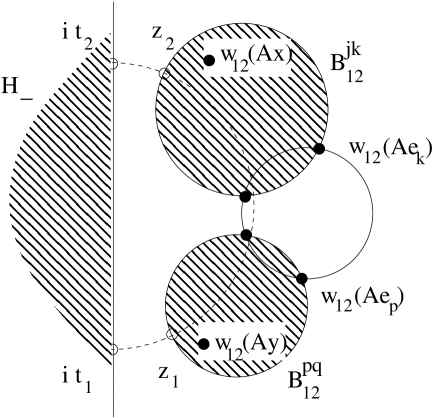
Figure 2: Bounding $\displaystyle{\rm diam}_{P}(E_{12})\leq d_{{{\mathbb{H}}}_{-}}(z_{1},z_{2})=\displaystyle\left|\log|[z_{1},z_{2};it_{1},it_{2}]|\right|$.

Similarly ${w_{12}}(Ay)\in B^{pq}_{12}$ for some indices p,q. By Corollary 6.7 the closure of these two disks either intersect directly or they intersect the closure of a 3rd disk, e.g. $B^{kp}_{12}$ in $N^{kp}_{12}(P)=\{w_{12}(Ae_{k}),w_{12}(Ae_{p})\}$. Therefore, (see Figure 2):

$$d_{\;\overline{{\rule[0.0pt]{0.0pt}{6.02777pt}{}}\mathbb{H}}{\rule[0.0pt]{0.0pt}{6.02777pt}{}}_{+}}({\widehat{w}}_{12}(Ax),{\widehat{w}}_{12}(Ay))\leq{\rm diam}_{\overline{{\rule[0.0pt]{0.0pt}{6.02777pt}{}}\mathbb{H}}{\rule[0.0pt]{0.0pt}{6.02777pt}{}}_{+}}(\widehat{B}^{jk}_{12})+{\rm diam}_{\overline{{\rule[0.0pt]{0.0pt}{6.02777pt}{}}\mathbb{H}}{\rule[0.0pt]{0.0pt}{6.02777pt}{}}_{+}}(\widehat{N_{12}^{kp}(P)})+{\rm diam}_{\overline{{\rule[0.0pt]{0.0pt}{6.02777pt}{}}\mathbb{H}}{\rule[0.0pt]{0.0pt}{6.02777pt}{}}_{+}}(\widehat{B}^{pq}_{12}).$$ (9.60)

Using the notation in Appendix A for diameters and distances, we obtain the bound

$$d_{\;\overline{{\rule[0.0pt]{0.0pt}{6.02777pt}{}}\mathbb{H}}{\rule[0.0pt]{0.0pt}{6.02777pt}{}}_{+}}({\widehat{w}}_{12}(Ax),{\widehat{w}}_{12}(Ay))\leq\Delta_{1}(N^{jk}_{12})\;+\;\Delta_{2}(N^{kp}_{12})\;+\;\Delta_{1}(N^{pq}_{12}).$$ (9.61)

For the second term we proceed along the same lines to get (for some other indices $j,k,p,q$):

$$d_{{\rule[0.0pt]{0.0pt}{6.32918pt}{}}{\mathbb{C}}^{*}}({\widehat{w}}_{12}(Ax),{\widehat{w}}_{12}(Ay))\ \leq \ {\rm diam}_{{\mathbb{C}}^{*}}(\widehat{B}^{jk}_{23})+{\rm diam}_{{\mathbb{C}}^{*}}(\widehat{N_{23}^{kp}(P)})+{\rm diam}_{{\mathbb{C}}^{*}}(\widehat{B}^{pq}_{23})$$ (9.62)

$$= \ \Delta_{3}(N^{jk}_{23})\ +\ \Delta_{4}(N^{kp}_{23})\ +\ \Delta_{3}(N^{pq}_{23})\;$$ (9.63)

Collecting the above estimates and taking sup over all possible 2 by 2 sub-matrices we obtain

$$d_{2}(Ax,Ay)=d_{{\mathbb{C}}^{*}}(u,v)\leq 4\Delta_{1}(A)+2\Delta_{2}(A)+2\Delta_{3}(A)+\Delta_{4}(A),$$ (9.64)

where $\Delta_{i}(A)=\sup_{T\in{\cal T}(A)}\Delta_{i}(T^{t})\;\in\;[0,+\infty]$, $i=1,2,3,4$. Since $u,v\in E$ were arbitrary we conclude that ${\rm diam}_{2}(A({{{K}}_{{\mathbb{C}},1}})^{*})\leq 4\Delta_{1}(A)+2\Delta_{2}(A)+2\Delta_{3}(A)+\Delta_{4}(A)\leq 9\Delta_{1}(A)$. With the hypothesis on $A$, $\Delta_{1}(A)\leq\delta_{1}(\theta)$ (see Definition 2.6). Using Theorem 7.2 we obtain the claimed Lipschitz inequality in Theorem 2.9 as well as the more refined estimate in (2.13).    

10 Proof of Theorem 2.10

The proof in [Rugh10, Theorem 3.6 and Theorem 3.7] carries over when we replace the ‘gauge’ by the present projective cross-ratio metric (see also [Dub09, Lemma 2.6 and Theorem 2.7]). The only missing part is the claim that $\nu\in{{{K}}^{\;{}^{\prime}}_{{\mathbb{C}}}}$ and that $\langle\nu,x\rangle\neq 0$ whenever $x\in{({{K}}_{{\mathbb{C}}})^{*}}$. Pick $m\in{K}_{{{\mathbb{R}}}}$ so that $\langle m,h\rangle=1$. ¿From (2.12) we get for $x\in X$, $n\geq 1$:

$$\left|\langle\lambda^{-n}(A^{\prime})^{n}m,x\rangle-\langle\nu,x\rangle\right|=\left|\langle m,\lambda^{-n}A^{n}x\rangle-\langle\nu,x\rangle\right|\leq C\eta_{1}(\theta)^{n-1}\|x\|$$ (10.65)

Here, $\lambda^{-n}(A^{\prime})^{n}m\in{{{K}}^{\;{}^{\prime}}_{{\mathbb{C}}}}$ so taking the $n\rightarrow\infty$ limit we deduce that $\nu\in{{{K}}^{\;{}^{\prime}}_{{\mathbb{C}}}}$. Fix $x\in{({{K}}_{{\mathbb{C}}})^{*}}$ and note that $d_{{{K}}_{{\mathbb{C}}}}(Ax,h)=d_{{{K}}_{{\mathbb{C}}}}(Ax,Ah)\leq\Delta(A)<+\infty$. From the definition of our metric it follows that for any $\mu\in{{{K}}^{\;{}^{\prime}}_{{\mathbb{C}}}}$ either $\langle\mu,Ax\rangle=\langle\mu,h\rangle=0$ or both are non-zero (so they have a finite ratio). since $\langle\nu,h\rangle=1$ (whence non-zero), we deduce that $\langle\nu,Ax\rangle=\lambda\langle\nu,Ax\rangle$ must be non-zero as well.    

11 Proof of Theorem 3.1 (for integral kernels)

We will need the following

Lemma 11.1

Let $(\Omega,\mu)$ be a $\sigma$-finite measure space, $1\leq p\leq+\infty$ and $1/q+1/p=1$. Let $f_{1},f_{2}\in L^{p}_{+}(\Omega,\mu)$ and suppose that $f_{1}f_{2}\geq 0$ a.e. Then $\|f_{1}\|_{p}+\|f_{2}\|_{p}\leq 2^{1/q}\|f_{1}+f_{2}\|$.

Proof: Using a $(q,p)$-Hölder inequality for ${{\mathbb{R}}}^{2}$ we have

$$\|f_{1}\|_{p}+\|f_{2}\|_{p}=(1,1)\cdot\left(\|f_{1}\|_{p},\|f_{2}\|_{p}\right)\leq 2^{1/q}\left({\rule[0.0pt]{0.0pt}{9.04166pt}{}}{\left\|{\rule[0.0pt]{0.0pt}{9.04166pt}{}}f_{1}\right\|}_{p}^{p}+\left\|{\rule[0.0pt]{0.0pt}{9.04166pt}{}}f_{2}\right\|_{p}^{p}\right)^{1/p}.$$

Our hypothesis implies that $|f_{1}|^{p}+|f_{2}|^{p}\leq|f_{1}+f_{2}|^{p}$ and the claim follows.   

In Theorem 3.1 we consider the space $X=L^{p}(\Omega,\mu)$. The real cone we use is ${K}_{{{\mathbb{R}}}}=L^{p}_{+}(\Omega,\mu)$. The dual (real) cone for $1\leq p<+\infty$ may be identified with ${{K}^{\;{}^{\prime}}_{{{\mathbb{R}}}}}=L^{q}_{+}(\Omega,\mu)$. When $p=\infty$, note that $L^{\infty}$ is the dual of $L^{1}$. It follows from the Goldstine Lemma (see e.g. [Bre83, lemme III.4]) that the unit ball in $L^{1}$ is weak-$*$ dense in $X^{\prime}$. Then also ${\cal M}=L^{1}_{+}(\Omega,\mu)$ is weak-$*$ dense in ${{K}^{\;{}^{\prime}}_{{{\mathbb{R}}}}}$ and this suffices for our purposes. So for any $1\leq p\leq+\infty$ we may consider ${\cal M}=L^{q}_{+}(\Omega,\mu)$ as a weak-$*$ generating set for the dual real cone. For $f\in X$ write $f=f_{+}-f_{-}$ with $f_{+},f_{-}\geq 0$ and $f_{+}\cdot f_{-}=0$. The above Lemma shows that $\|f_{+}\|+\|f_{-}\|\leq 2^{1/q}\|f\|$ so ${K}_{{{\mathbb{R}}}}$ is regenerating with a constant $g=2^{1/q}\leq q$. By [Rugh10, Lemma 4.2] we have the following bound for the sectional aperture for ${{{K}}_{{\mathbb{C}}}}$:

$$\kappa({{{K}}_{{\mathbb{C}}}})=\sup_{f_{1},f_{2}\in{({{K}}_{{\mathbb{C}}})^{*}}}\frac{\|f_{1}\|+\|f_{2}\|}{\|f_{1}+f_{2}\|}\leq 2^{1/q}\leq 2.$$

We need to verify that ${\cal T}(L)\subset{\Gamma}{\rule[0.0pt]{0.0pt}{8.61108pt}{}}_{+}\left(\theta\right)$. So pick $f_{1},f_{2}\in{K}_{{{\mathbb{R}}}}^{*}=\left(L^{q}_{+}(\Omega,\mu)\right)^{*}$ and $g_{1},g_{2}\in{\cal M}=\left(L^{p}_{+}(\Omega,\mu)\right)^{*}$. We denote

$$A_{ij}=\langle g_{i},Lf_{j}\rangle=\int\int f_{j}(x)k(x,y)g_{i}(y).$$ (11.66)

Here and in the following, when the meaning is clear from the context we omit the domain and the measure used for the integrals. Abbreviating Using the properties of $N_{x_{1},x_{2};y_{1},y_{2}}$ and abbreviating $k_{ij}=k(x_{i},y_{j})$, $i,j=1,2$ for its matrix elements we get the following inequality:

$$\frac{1}{\theta}\left|A_{11}A_{22}-A_{12}A_{21}\right|\ \ \ \ \$$ (11.67)

$$= \frac{1}{\theta}\left|\int\int\int\int f_{1}(x_{1})f_{2}(x_{2})g_{1}(y_{1})g_{2}(y_{2})\left(k_{11}k_{22}-k_{12}k_{21}\right)\right|$$ (11.68)

$$\leq \int\int\int\int f_{1}(x_{1})f_{2}(x_{2})g_{1}(y_{1})g_{2}(y_{2})\ {\rm Re\,}\left(k_{11}\overline{\rule[0.0pt]{0.0pt}{8.94441pt}{}{k}}_{22}+k_{12}\overline{\rule[0.0pt]{0.0pt}{8.94441pt}{}{k}}_{21}\right)$$ (11.69)

$$= {\rm Re\,}\;\left(A_{11}\overline{\rule[0.0pt]{0.0pt}{8.83328pt}{}{A}}_{22}+A_{12}\overline{\rule[0.0pt]{0.0pt}{8.83328pt}{}{A}}_{21}\right).$$ (11.70)

A similar calculation also shows that ${\rm Re\,}\;\left(A_{11}\overline{\rule[0.0pt]{0.0pt}{8.83328pt}{}{A}}_{22}+A_{12}\overline{\rule[0.0pt]{0.0pt}{8.83328pt}{}{A}}_{21}\right)>0$ since the product $f_{1}f_{2}g_{1}g_{2}$ do not vanish identically and ${\rm Re\,}\left(k_{11}\overline{\rule[0.0pt]{0.0pt}{8.94441pt}{}{k}}_{22}+k_{12}\overline{\rule[0.0pt]{0.0pt}{8.94441pt}{}{k}}_{21}\right)>0$ (a.e.). This shows that the matrix $A=(A_{ij})_{i,j=1,2}\in{\Gamma}{\rule[0.0pt]{0.0pt}{8.61108pt}{}}_{+}\left(\theta\right)$. We may then apply Theorem 2.10.   

12 Variational formulae. Proofs of Theorem 4.2 and 4.3

We consider again the case then $X_{1}=X_{2}$ and the cones are the same (so indices are omitted). For $x\in X$, $\mu\in X^{\prime}$ we write $\ker x=\{m\in X^{\prime}:\langle m,x\rangle=0\}$

Lemma 12.1

The pre-order in Definition 2.1 is a closed relation. The operator $A$ in Theorem 4.2 and 4.3 preserves the pre-order.

Proof: That the relation is closed follows from continuity of each linear functional $\mu\in{{{K}}^{\;{}^{\prime}}_{{\mathbb{C}}}}$. By Theorem 2.7, $A^{\prime}({{{K}}^{\;{}^{\prime}}_{{\mathbb{C}}}})\subset{{{K}}^{\;{}^{\prime}}_{{\mathbb{C}}}}$. So suppose $x\preceq y$ and let $\mu\in{{{K}}^{\;{}^{\prime}}_{{\mathbb{C}}}}$. Then $|\langle\mu,Ax\rangle|=|\langle A^{\prime}\mu,x\rangle|\leq|\langle A^{\prime}\mu,y\rangle|=|\langle\mu,Ay\rangle|$, since $A^{\prime}\mu\in{{{K}}^{\;{}^{\prime}}_{{\mathbb{C}}}}$.    

Lemma 12.2

We have the following lower bound for the spectral radius of $A$:

$$r_{\rm sp}(A)\geq\sup_{x\in{({{K}}_{{\mathbb{C}}})^{*}}}\alpha(Ax,x)$$ (12.71)

Proof: Let $x\in{({{K}}_{{\mathbb{C}}})^{*}}$ and $r\leq\alpha(Ax,x)$ so that $Ax\succeq rx$. Since $A$ preserves the pre-order we may iterate this relation and obtain $r^{n}x\preceq A^{n}x$, $n\geq 1$. Let $\mu\in{{{K}}^{\;{}^{\prime}}_{{\mathbb{C}}}}$ be such that $\langle\mu,x\rangle\neq 0$. Then

$$0<r^{n}|\langle\mu,x\rangle|\leq|\langle\mu,A^{n}x\rangle|\leq\|A^{n}\|\;\|\mu\|\;\|x\|,\ \ n\geq 1$$ (12.72)

Since $\mu$ and $x$ are fixed we get $r_{\rm sp}(A)\geq r$.    

Let $M=\left(\!\begin{array}[]{cc}a&b\\ c&d\end{array}\!\right)$ and assume that ${\rm Re\,}a\overline{\rule[0.0pt]{0.0pt}{8.94441pt}{}{b}}\geq 0$, ${\rm Re\,}c\overline{\rule[0.0pt]{0.0pt}{8.94441pt}{}{d}}\geq 0$. We define $\displaystyle F=M\left(\overline{{\rule[0.0pt]{0.0pt}{8.61108pt}{}}\mathbb{C}}{\rule[0.0pt]{0.0pt}{8.61108pt}{}}_{+}^{\hskip 1.05487pt2}\right)$ and let $\widehat{F}=\pi\left(F^{*}\right)$ be the projection on the sphere $\widehat{{\mathbb{C}}}$. Let $\phi(M)$ and $\Phi(M)$ be as in in Definition 4.1.

Lemma 12.3

We then have

$$\sup\left|\widehat{F}\right|=\Phi(M)\ \ \mbox{and}\ \ \inf\left|\widehat{F}\right|=\phi(M)\ .$$

Proof: When $ad-bc\neq 0$ we let $\displaystyle R(z)=\frac{az+b}{cz+d}$ be the associated Möbius transformation. $\widehat{F}$ is then the set $R(\overline{{\rule[0.0pt]{0.0pt}{8.61108pt}{}}\mathbb{H}}{\rule[0.0pt]{0.0pt}{8.61108pt}{}}_{+})$ which is either a a disk or a halfplane. When ${\rm Re\,}c\overline{\rule[0.0pt]{0.0pt}{8.94441pt}{}{d}}>0$ it is a disk and the formulae (A.77) for the center $C$ and radius $r$ are still valid in this case. Then $\sup|\widehat{F}|$ is simply the expression for $|C|+r$. For the second equality note that $\widehat{F}$ is disjoint from the origin when ${\rm Re\,}a\overline{\rule[0.0pt]{0.0pt}{8.94441pt}{}{b}}>0$ (using Lemma 6.5). So the origin is not in the open disk $R(\overset{\circ}{\mathbb{H}}{\rule[0.0pt]{0.0pt}{8.61108pt}{}}_{+})$, even when ${\rm Re\,}a\overline{\rule[0.0pt]{0.0pt}{8.94441pt}{}{b}}\geq 0$. It follows that $|C|\geq r$ so we have the expression $\inf|\widehat{F}|=|C|-r$. We have that $|a\overline{\rule[0.0pt]{0.0pt}{8.94441pt}{}{d}}+b\overline{\rule[0.0pt]{0.0pt}{6.30551pt}{}{c}}|^{2}-|ad-bc|^{2}=\;2{\rm Re\,}a\overline{\rule[0.0pt]{0.0pt}{8.94441pt}{}{b}}\ 2{\rm Re\,}c\overline{\rule[0.0pt]{0.0pt}{8.94441pt}{}{d}}$. The expression $|C|^{2}-r^{2}={{\rm Re\,}a\overline{\rule[0.0pt]{0.0pt}{8.94441pt}{}{b}}}/{{\rm Re\,}c\overline{\rule[0.0pt]{0.0pt}{8.94441pt}{}{d}}}\geq 0$ and $\inf|\widehat{F}|=|C|-r$ then leads to the second formula. The case of a halfplane, i.e.  ${\rm Re\,}c\overline{\rule[0.0pt]{0.0pt}{8.94441pt}{}{d}}=0$, follows by taking limits. When $ad-bc=0$ the image $M(\overline{{\rule[0.0pt]{0.0pt}{8.61108pt}{}}\mathbb{C}}{\rule[0.0pt]{0.0pt}{8.61108pt}{}}_{+}^{\hskip 1.05487pt2})$ is one-dimensional and $\widehat{F}$ therefore a single point given by $a/c\in\widehat{{\mathbb{C}}}$ (or $b/d$ if both $a$ and $c$ should vanish). When $M$ is the zero-matrix, $\widehat{F}$ is empty and we set $\sup\emptyset=\Phi(0)=0$ and $\inf\emptyset=\phi(0)=+\infty$.    

Proof of Theorem 4.2.  For $x\in{({{K}}_{{\mathbb{C}}})^{*}}$ we have $Ax\in{{{K}}_{{\mathbb{C}}}}$. If $Ax=0$ then $\alpha(x,Ax)=0$. So consider the case when $Ax\neq 0$. We denote $M_{m_{1}m_{2}}=T(m_{1},m_{2};Ax,x)$, $m_{1},m_{2}\in{\cal M}$ and write $F_{m_{1}m_{2}}=M_{m_{1}m_{2}}\left(\overline{{\rule[0.0pt]{0.0pt}{8.61108pt}{}}\mathbb{C}}{\rule[0.0pt]{0.0pt}{8.61108pt}{}}_{+}^{\hskip 1.05487pt2}\right)$. By the previous lemma and (8.53) we have

$$\alpha(Ax,x)=\inf\left|\widehat{E}(Ax,x)\right|=\inf_{m_{1},m_{2}\in{\cal M}}\left|\widehat{F}_{m_{1}\,m_{2}}\right|=\inf_{m_{1},m_{2}\in{\cal M}}\phi\left(M_{m_{1}\,m_{2}}\right).\ \raisebox{2.58334pt}{\framebox[3.87495pt]{ \rule[0.0pt]{0.0pt}{2.15277pt} }}$$ (12.73)

Proof of Theorem 4.3.  Under the hypotheses of Theorem 2.10 we will show the following identity:

$$r_{\rm sp}(A)=\sup_{x\in{({{K}}_{{\mathbb{C}}})^{*}}}\alpha(Ax,x)=\inf_{x\in{({{K}}_{{\mathbb{C}}})^{*}}}\beta(Ax,x)$$ (12.74)

We will make use of the fact that the dual eigenvector $\lambda\nu=A\nu$ does not vanish on ${({{K}}_{{\mathbb{C}}})^{*}}$. So for every $x\in{({{K}}_{{\mathbb{C}}})^{*}}$ we have: $\displaystyle\alpha(Ax,x)=\inf|\widehat{E}(Ax,x)|\leq\left|\frac{\langle\nu,Ax\rangle}{\langle\nu,x\rangle}\right|=|\lambda|=r_{\rm sp}(A)$. Combining with the previous Theorem we obtain the first equality.

If $x\in{({{K}}_{{\mathbb{C}}})^{*}}$ and $r>0$ are such that $Ax\preceq rx$ then applying $\nu$ we get $|\lambda||\langle\nu,x\rangle|\leq r|\langle\nu,x\rangle|$. Since $\langle\nu,x\rangle\neq 0$ we conclude that $r_{\rm sp}(A)\leq\beta(Ax,x)$ for any $x\in{({{K}}_{{\mathbb{C}}})^{*}}$. For $x=h$ we have equality and thus (12.74). Repeating the steps in the previous proof for calculating $\alpha$ and similarly for $\beta$ we obtain the equalities in Theorem 4.3. Also when $x=h$ (the right eigenvector) we have $\alpha(Ah,h)=\beta(Ah,h)=|\lambda|\alpha(h,h)=|\lambda|=r_{\rm sp}(A)$.    

Remark 12.4

Note that the conclusion of Theorem 4.3 may fail if $A$ is cone-preserving but not a strict contraction. For example, $A=\left(\!\begin{array}[]{cc}2&0\\ 0&1\end{array}\!\right)$ preserves $(\overline{{\rule[0.0pt]{0.0pt}{8.61108pt}{}}\mathbb{C}}{\rule[0.0pt]{0.0pt}{8.61108pt}{}}_{+}^{\hskip 1.05487pt2})^{*}$ but $\inf\beta(Ax,x)=1$.

Appendix A Contractions of 2 by 2 matrices

Definition A.1

Define the following sets of $2\times 2$ matrices:

$$\overset{\circ}{\Gamma}{\rule[0.0pt]{0.0pt}{8.61108pt}{}}_{+}=\left\{\left(\!\begin{array}[]{cc}a&b\\ c&d\end{array}\!\right)\in M_{2}({\mathbb{C}}):|ad-bc|<{\rm Re\,}(a\overline{\rule[0.0pt]{0.0pt}{8.94441pt}{}{d}}+b\overline{\rule[0.0pt]{0.0pt}{6.30551pt}{}{c}}),\ \ \ a\,\overline{\rule[0.0pt]{0.0pt}{8.94441pt}{}{b}},\ \ a\,\overline{\rule[0.0pt]{0.0pt}{6.30551pt}{}{c}},\ \ b\,\overline{\rule[0.0pt]{0.0pt}{8.94441pt}{}{d}},\ \ c\,\overline{\rule[0.0pt]{0.0pt}{8.94441pt}{}{d}}\;\in\overset{\circ}{\mathbb{H}}{\rule[0.0pt]{0.0pt}{8.61108pt}{}}_{+}\right\}.$$

$$\overline{{\rule[0.0pt]{0.0pt}{8.61108pt}{}}\Gamma}{\rule[0.0pt]{0.0pt}{8.61108pt}{}}_{+}=\left\{\left(\!\begin{array}[]{cc}a&b\\ c&d\end{array}\!\right)\in M_{2}({\mathbb{C}}):|ad-bc|\leq{\rm Re\,}(a\overline{\rule[0.0pt]{0.0pt}{8.94441pt}{}{d}}+b\overline{\rule[0.0pt]{0.0pt}{6.30551pt}{}{c}}),\ \ \ a\,\overline{\rule[0.0pt]{0.0pt}{8.94441pt}{}{b}},\ \ a\,\overline{\rule[0.0pt]{0.0pt}{6.30551pt}{}{c}},\ \ b\,\overline{\rule[0.0pt]{0.0pt}{8.94441pt}{}{d}},\ \ c\,\overline{\rule[0.0pt]{0.0pt}{8.94441pt}{}{d}}\;\in\overline{{\rule[0.0pt]{0.0pt}{8.61108pt}{}}\mathbb{H}}{\rule[0.0pt]{0.0pt}{8.61108pt}{}}_{+}\right\}.$$

For the standard topology on $M_{2}({\mathbb{C}})$, $\overset{\circ}{\Gamma}{\rule[0.0pt]{0.0pt}{8.61108pt}{}}_{+}$ is the interior of $\overline{{\rule[0.0pt]{0.0pt}{8.61108pt}{}}\Gamma}{\rule[0.0pt]{0.0pt}{8.61108pt}{}}_{+}$ and $\overline{{\rule[0.0pt]{0.0pt}{8.61108pt}{}}\Gamma}{\rule[0.0pt]{0.0pt}{8.61108pt}{}}_{+}$ is the closure of $\overset{\circ}{\Gamma}{\rule[0.0pt]{0.0pt}{8.61108pt}{}}_{+}$.

We have the following characterisation:

Proposition A.2

$M^{t}$ denotes the transposed matrix of $M$.

1. $M\in\overset{\circ}{\Gamma}{\rule[0.0pt]{0.0pt}{8.61108pt}{}}_{+}$     iff  $M:(\overline{{\rule[0.0pt]{0.0pt}{8.61108pt}{}}\mathbb{C}}{\rule[0.0pt]{0.0pt}{8.61108pt}{}}_{+}^{\hskip 1.05487pt2})^{*}\rightarrow\overset{\circ}{\mathbb{C}}{\rule[0.0pt]{0.0pt}{8.61108pt}{}}_{+}^{\hskip 0.60275pt2}$  iff  $M^{t}:(\overline{{\rule[0.0pt]{0.0pt}{8.61108pt}{}}\mathbb{C}}{\rule[0.0pt]{0.0pt}{8.61108pt}{}}_{+}^{\hskip 1.05487pt2})^{*}\rightarrow\overset{\circ}{\mathbb{C}}{\rule[0.0pt]{0.0pt}{8.61108pt}{}}_{+}^{\hskip 0.60275pt2}$  iff  $\forall\;u,v\in(\overline{{\rule[0.0pt]{0.0pt}{8.61108pt}{}}\mathbb{C}}{\rule[0.0pt]{0.0pt}{8.61108pt}{}}_{+}^{\hskip 1.05487pt2})^{*}:\langle u,Mv\rangle\neq 0$.

2. $M\in\overline{{\rule[0.0pt]{0.0pt}{8.61108pt}{}}\Gamma}{\rule[0.0pt]{0.0pt}{8.61108pt}{}}_{+}$     iff  $M:\overline{{\rule[0.0pt]{0.0pt}{8.61108pt}{}}\mathbb{C}}{\rule[0.0pt]{0.0pt}{8.61108pt}{}}_{+}^{\hskip 1.05487pt2}\rightarrow\overline{{\rule[0.0pt]{0.0pt}{8.61108pt}{}}\mathbb{C}}{\rule[0.0pt]{0.0pt}{8.61108pt}{}}_{+}^{\hskip 1.05487pt2}$   and   $M^{t}:\overline{{\rule[0.0pt]{0.0pt}{8.61108pt}{}}\mathbb{C}}{\rule[0.0pt]{0.0pt}{8.61108pt}{}}_{+}^{\hskip 1.05487pt2}\rightarrow\overline{{\rule[0.0pt]{0.0pt}{8.61108pt}{}}\mathbb{C}}{\rule[0.0pt]{0.0pt}{8.61108pt}{}}_{+}^{\hskip 1.05487pt2}$

3. If $M:\overline{{\rule[0.0pt]{0.0pt}{8.61108pt}{}}\mathbb{C}}{\rule[0.0pt]{0.0pt}{8.61108pt}{}}_{+}^{\hskip 1.05487pt2}\rightarrow\overline{{\rule[0.0pt]{0.0pt}{8.61108pt}{}}\mathbb{C}}{\rule[0.0pt]{0.0pt}{8.61108pt}{}}_{+}^{\hskip 1.05487pt2}$   and   $\det M\neq 0$   then  $M\in\overline{{\rule[0.0pt]{0.0pt}{8.61108pt}{}}\Gamma}{\rule[0.0pt]{0.0pt}{8.61108pt}{}}_{+}$.

Proof: First note that the equivalence of the last three conditions in (1) follows from Lemma 6.5 and the symmetry of the last expression. It is convenient to distinguish cases according to the rank of $M$. The zero-matrix is in $\overline{{\rule[0.0pt]{0.0pt}{8.61108pt}{}}\Gamma}{\rule[0.0pt]{0.0pt}{8.61108pt}{}}_{+}$ and not in $\overset{\circ}{\Gamma}{\rule[0.0pt]{0.0pt}{8.61108pt}{}}_{+}$ which is consistent with (1) and (2). So let us consider the case of rank $M=1$: We may then write

$$M=\left(\!\begin{array}[]{cc}a&b\\ c&d\end{array}\!\right)=\left(\!\begin{array}[]{c}\alpha_{1}\\ \alpha_{2}\end{array}\!\right)\left(\!\begin{array}[]{cc}\beta_{1}&\beta_{2}\end{array}\!\right)=\left(\!\begin{array}[]{cc}\alpha_{1}\beta_{1}&\alpha_{1}\beta_{2}\\ \alpha_{2}\beta_{1}&\alpha_{2}\beta_{2}\end{array}\!\right).$$

In order to show (1) we note that $\forall\;u,v\in(\overline{{\rule[0.0pt]{0.0pt}{8.61108pt}{}}\mathbb{C}}{\rule[0.0pt]{0.0pt}{8.61108pt}{}}_{+}^{\hskip 1.05487pt2})^{*}:\langle u,Mv\rangle=\langle u,\alpha\rangle\langle\beta,v\rangle\neq 0$ is equivalent to $\alpha,\beta\in{\overset{\circ}{\mathbb{C}}{\rule[0.0pt]{0.0pt}{8.61108pt}{}}_{+}^{\hskip 0.60275pt2}}$ which is the same as $a\,\overline{\rule[0.0pt]{0.0pt}{8.94441pt}{}{b}},\ a\,\overline{\rule[0.0pt]{0.0pt}{6.30551pt}{}{c}},\ c\,\overline{\rule[0.0pt]{0.0pt}{8.94441pt}{}{b}},\ c\,\overline{\rule[0.0pt]{0.0pt}{8.94441pt}{}{d}}\;\in\overset{\circ}{\mathbb{H}}{\rule[0.0pt]{0.0pt}{8.61108pt}{}}_{+}$. In this case the inequality  ${\rm Re\,}(a\overline{\rule[0.0pt]{0.0pt}{8.94441pt}{}{d}}+b\overline{\rule[0.0pt]{0.0pt}{6.30551pt}{}{c}})=2{\rm Re\,}\alpha_{1}\overline{\alpha}_{2}\ \ {\rm Re\,}\beta_{1}\overline{\beta}_{2}>0=|ad-bc|$ is automatic so we get the equivalence with $M$ being in $\overset{\circ}{\Gamma}{\rule[0.0pt]{0.0pt}{8.61108pt}{}}_{+}$. To see (2) consider the vectors $\left(\!\begin{array}[]{c}a\\ c\end{array}\!\right)$, $\left(\!\begin{array}[]{c}b\\ d\end{array}\!\right)$, $\left(\!\begin{array}[]{c}a\\ b\end{array}\!\right)$ and $\left(\!\begin{array}[]{c}c\\ d\end{array}\!\right)$ which are the images of the ‘polar’ vectors $\left(\!\begin{array}[]{c}1\\ 0\end{array}\!\right),\left(\!\begin{array}[]{c}0\\ 1\end{array}\!\right)\in\overline{{\rule[0.0pt]{0.0pt}{8.61108pt}{}}\mathbb{C}}{\rule[0.0pt]{0.0pt}{8.61108pt}{}}_{+}^{\hskip 1.05487pt2}$ by $M$ and $M^{t}$. These vectors belong to $\overline{{\rule[0.0pt]{0.0pt}{8.61108pt}{}}\mathbb{C}}{\rule[0.0pt]{0.0pt}{8.61108pt}{}}_{+}^{\hskip 1.05487pt2}$ precisley when the real parts of $a\overline{\rule[0.0pt]{0.0pt}{8.94441pt}{}{b}},c\overline{\rule[0.0pt]{0.0pt}{8.94441pt}{}{d}},a\overline{\rule[0.0pt]{0.0pt}{6.30551pt}{}{c}},b\overline{\rule[0.0pt]{0.0pt}{8.94441pt}{}{d}}$ are non-negative. The condition ${\rm Re\,}(a\overline{\rule[0.0pt]{0.0pt}{8.94441pt}{}{d}}+b\overline{\rule[0.0pt]{0.0pt}{6.30551pt}{}{c}})=2{\rm Re\,}\alpha_{1}\overline{\alpha}_{2}\ \ {\rm Re\,}\beta_{1}\overline{\beta}_{2}\geq 0=|ad-bc|$ is automatically satisfied and since the images of $M$ and $M^{t}$ are one-dimensional we obtain the equivalence in (2).

Consider then the case Rank $M=2$, i.e. $ad-bc\neq 0$. We fist show (1) in this case. The images of the polar points are in $\overset{\circ}{\mathbb{C}}{\rule[0.0pt]{0.0pt}{8.61108pt}{}}_{+}^{\hskip 0.60275pt2}$ precisely when ${\rm Re\,}a\overline{\rule[0.0pt]{0.0pt}{6.30551pt}{}{c}}>0$ and ${\rm Re\,}b\overline{\rule[0.0pt]{0.0pt}{8.94441pt}{}{d}}>0$. Note that $\displaystyle M\left((\overline{{\rule[0.0pt]{0.0pt}{8.61108pt}{}}\mathbb{C}}{\rule[0.0pt]{0.0pt}{8.61108pt}{}}_{+}^{\hskip 1.05487pt2})^{*}\right)\subset\overset{\circ}{\mathbb{C}}{\rule[0.0pt]{0.0pt}{8.61108pt}{}}_{+}^{\hskip 0.60275pt2}$ so the image of $\displaystyle(\overline{{\rule[0.0pt]{0.0pt}{8.61108pt}{}}\mathbb{C}}{\rule[0.0pt]{0.0pt}{8.61108pt}{}}_{+}^{\hskip 1.05487pt2})^{*}$ does not contain the polar vectors. The inverse of $M$ is proportional to the matrix $\left(\!\begin{array}[]{rr}d&-b\\ -c&a\end{array}\!\right)$ and it should therefore map the polar points to (non-zero) vectors in the complement of $\overline{{\rule[0.0pt]{0.0pt}{8.61108pt}{}}\mathbb{C}}{\rule[0.0pt]{0.0pt}{8.61108pt}{}}_{+}^{\hskip 1.05487pt2}$. This translates into ${\rm Re\,}d(-\overline{\rule[0.0pt]{0.0pt}{6.30551pt}{}{c}})<0$ and ${\rm Re\,}(-b)\overline{\rule[0.0pt]{0.0pt}{6.30551pt}{}{a}}<0$ or equivalently ${\rm Re\,}c\overline{\rule[0.0pt]{0.0pt}{8.94441pt}{}{d}}>0$ and ${\rm Re\,}a\overline{\rule[0.0pt]{0.0pt}{8.94441pt}{}{b}}>0$. To show the last condition we associate to $M$ the Möbius map $\displaystyle R(z)=\frac{az+b}{cz+d}$ which acts upon the Riemann sphere $\widehat{{\mathbb{C}}}$. Since ${\rm Re\,}c\,\overline{\rule[0.0pt]{0.0pt}{8.94441pt}{}{d}}>0$ it follows that $R$ maps $\overline{{\rule[0.0pt]{0.0pt}{8.61108pt}{}}\mathbb{H}}{\rule[0.0pt]{0.0pt}{8.61108pt}{}}_{+}\cup\{\infty\}$ onto a closed disk in ${\mathbb{C}}$. We compute its center and radius as follows. For $z,z_{0}\in\widehat{{\mathbb{C}}}$:

$$R(z)-R(z_{0}) = \frac{az+b}{cz+d}-\frac{az_{0}+b}{cz_{0}+d}=\frac{(ad-bc)(z-z_{0})}{(cz_{0}+d)(cz+d)}$$ (A.75)

$$= \frac{(ad-bc)}{c{z_{0}}\overline{\rule[0.0pt]{0.0pt}{6.30551pt}{}{c}}+d\overline{\rule[0.0pt]{0.0pt}{6.30551pt}{}{c}}}\times\frac{\overline{\rule[0.0pt]{0.0pt}{6.30551pt}{}{c}}{z}-\overline{\rule[0.0pt]{0.0pt}{6.30551pt}{}{c}}{z_{0}}}{cz+d}.$$ (A.76)

Setting $z_{0}=\overline{\rule[0.0pt]{0.0pt}{8.94441pt}{}{d}}/\overline{\rule[0.0pt]{0.0pt}{6.30551pt}{}{c}}$ we get:

$$R(z)-R(\overline{\rule[0.0pt]{0.0pt}{8.94441pt}{}{d}}/\overline{\rule[0.0pt]{0.0pt}{6.30551pt}{}{c}})=\frac{(ad-bc)}{c\overline{\rule[0.0pt]{0.0pt}{8.94441pt}{}{d}}+d\overline{\rule[0.0pt]{0.0pt}{6.30551pt}{}{c}}}\times\frac{\overline{\rule[0.0pt]{0.0pt}{6.30551pt}{}{c}}{z}-\overline{\rule[0.0pt]{0.0pt}{8.94441pt}{}{d}}}{cz+d}.$$

The image of ${\rm Re\,}z\geq 0$ is then the closed disk whose center and radius are given by

$$C=R(\overline{\rule[0.0pt]{0.0pt}{8.94441pt}{}{d}}/\overline{\rule[0.0pt]{0.0pt}{6.30551pt}{}{c}})=\frac{(a\overline{\rule[0.0pt]{0.0pt}{8.94441pt}{}{d}}+b\overline{\rule[0.0pt]{0.0pt}{6.30551pt}{}{c}})}{c\overline{\rule[0.0pt]{0.0pt}{8.94441pt}{}{d}}+d\overline{\rule[0.0pt]{0.0pt}{6.30551pt}{}{c}}}\ \ \mbox{and}\ \ r=\frac{\left|(ad-bc)\right|}{c\overline{\rule[0.0pt]{0.0pt}{8.94441pt}{}{d}}+d\overline{\rule[0.0pt]{0.0pt}{6.30551pt}{}{c}}}.$$ (A.77)

Therefore, $R$ maps $\overline{{\rule[0.0pt]{0.0pt}{8.61108pt}{}}\mathbb{H}}{\rule[0.0pt]{0.0pt}{8.61108pt}{}}_{+}$ into the interior of $\overset{\circ}{\mathbb{H}}{\rule[0.0pt]{0.0pt}{8.61108pt}{}}_{+}$ precisely when ${\rm Re\,}C>r$ and since ${\rm Re\,}c\,\overline{\rule[0.0pt]{0.0pt}{8.94441pt}{}{d}}>0$ this translates into the stated condition that $M\in\overset{\circ}{\Gamma}{\rule[0.0pt]{0.0pt}{8.61108pt}{}}_{+}$.

In order to show (2) and (3) (recall that here $\det M\neq 0$) we will use a continuity argument. When $M:\overline{{\rule[0.0pt]{0.0pt}{8.61108pt}{}}\mathbb{C}}{\rule[0.0pt]{0.0pt}{8.61108pt}{}}_{+}^{\hskip 1.05487pt2}\rightarrow\overline{{\rule[0.0pt]{0.0pt}{8.61108pt}{}}\mathbb{C}}{\rule[0.0pt]{0.0pt}{8.61108pt}{}}_{+}^{\hskip 1.05487pt2}$ and $\det M\neq 0$ then also $M:(\overline{{\rule[0.0pt]{0.0pt}{8.61108pt}{}}\mathbb{C}}{\rule[0.0pt]{0.0pt}{8.61108pt}{}}_{+}^{\hskip 1.05487pt2})^{*}\rightarrow(\overline{{\rule[0.0pt]{0.0pt}{8.61108pt}{}}\mathbb{C}}{\rule[0.0pt]{0.0pt}{8.61108pt}{}}_{+}^{\hskip 1.05487pt2})^{*}$. If we post-compose with $N_{\epsilon}=\left(\!\begin{array}[]{cc}1&\epsilon\\ \epsilon&1\end{array}\!\right)$, $\epsilon\in(0,1)$ (which maps $(\overline{{\rule[0.0pt]{0.0pt}{8.61108pt}{}}\mathbb{C}}{\rule[0.0pt]{0.0pt}{8.61108pt}{}}_{+}^{\hskip 1.05487pt2})^{*}$ into $\overset{\circ}{\mathbb{C}}{\rule[0.0pt]{0.0pt}{8.61108pt}{}}_{+}^{\hskip 0.60275pt2}$) then $N_{\epsilon}M:(\overline{{\rule[0.0pt]{0.0pt}{8.61108pt}{}}\mathbb{C}}{\rule[0.0pt]{0.0pt}{8.61108pt}{}}_{+}^{\hskip 1.05487pt2})^{*}\rightarrow\overset{\circ}{\mathbb{C}}{\rule[0.0pt]{0.0pt}{8.61108pt}{}}_{+}^{\hskip 0.60275pt2}$ so the product belongs to $\overset{\circ}{\Gamma}{\rule[0.0pt]{0.0pt}{8.61108pt}{}}_{+}$ by (1). As $\epsilon\rightarrow 0$ we conclude that $M\in\overline{{\rule[0.0pt]{0.0pt}{8.61108pt}{}}\Gamma}{\rule[0.0pt]{0.0pt}{8.61108pt}{}}_{+}$ (thus showing (3)). Any $M\in\overline{{\rule[0.0pt]{0.0pt}{8.61108pt}{}}\Gamma}{\rule[0.0pt]{0.0pt}{8.61108pt}{}}_{+}$ may be approximated by matrices in $\overset{\circ}{\Gamma}{\rule[0.0pt]{0.0pt}{8.61108pt}{}}_{+}$ so taking closure we get the reverse implication in (2).    

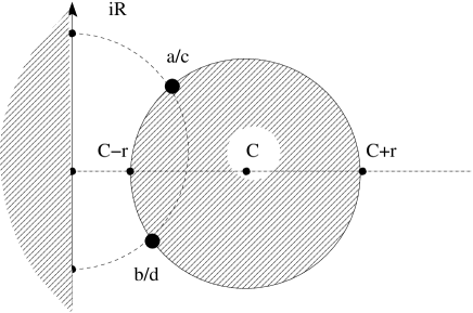
Figure 3: Contraction numbers.

A matrix $M\in\overset{\circ}{\Gamma}{\rule[0.0pt]{0.0pt}{8.61108pt}{}}_{+}$ is a strict contraction of $(\overline{{\rule[0.0pt]{0.0pt}{8.61108pt}{}}\mathbb{C}}{\rule[0.0pt]{0.0pt}{8.61108pt}{}}_{+}^{\hskip 1.05487pt2})^{*}$. In particular the image of any $(\overline{{\rule[0.0pt]{0.0pt}{8.61108pt}{}}\mathbb{C}}{\rule[0.0pt]{0.0pt}{8.61108pt}{}}_{+}^{\hskip 1.05487pt2})^{*}$ is never the zero vector (even when $\det M=0$). We may therefore associate to such a matrix 4 contraction numbers related to the way the associated linear fractional map contracts the cross-ratio metric.

Proposition A.3

Consider a matrix $M\in\overset{\circ}{\Gamma}{\rule[0.0pt]{0.0pt}{8.61108pt}{}}_{+}$. Let $R$ be the linear fractional map associated to $M$. We have the following formulae for diameters associated with the matrix:

1. $\displaystyle\Delta_{1}(M)\equiv{\rm diam}_{\overline{{\rule[0.0pt]{0.0pt}{6.02777pt}{}}\mathbb{H}}{\rule[0.0pt]{0.0pt}{6.02777pt}{}}_{+}}\left(R({\overline{{\rule[0.0pt]{0.0pt}{8.61108pt}{}}\mathbb{H}}{\rule[0.0pt]{0.0pt}{8.61108pt}{}}_{+}})\right)=\log\frac{{\rm Re\,}(a\overline{\rule[0.0pt]{0.0pt}{8.94441pt}{}{d}}+b\overline{\rule[0.0pt]{0.0pt}{6.30551pt}{}{c}})+|ad-bc|}{{\rm Re\,}(a\overline{\rule[0.0pt]{0.0pt}{8.94441pt}{}{d}}+b\overline{\rule[0.0pt]{0.0pt}{6.30551pt}{}{c}})-|ad-bc|}$

2. $\displaystyle\Delta_{2}(M)\equiv d_{\overline{{\rule[0.0pt]{0.0pt}{6.02777pt}{}}\mathbb{H}}{\rule[0.0pt]{0.0pt}{6.02777pt}{}}_{+}}\left(R(0),R(\infty)\right)=\log\frac{|a\overline{\rule[0.0pt]{0.0pt}{8.94441pt}{}{d}}+\overline{\rule[0.0pt]{0.0pt}{8.94441pt}{}{b}}c|+|ad-bc|}{|a\overline{\rule[0.0pt]{0.0pt}{8.94441pt}{}{d}}+\overline{\rule[0.0pt]{0.0pt}{8.94441pt}{}{b}}c|-|ad-bc|}$

3. $\displaystyle\Delta_{3}(M)\equiv{\rm diam}_{{\mathbb{C}}^{*}}\left(R(\overline{{\rule[0.0pt]{0.0pt}{8.61108pt}{}}\mathbb{H}}{\rule[0.0pt]{0.0pt}{8.61108pt}{}}_{+})\right)=\Delta_{2}(M^{t})=\log\frac{|a\overline{\rule[0.0pt]{0.0pt}{8.94441pt}{}{d}}+b\overline{\rule[0.0pt]{0.0pt}{6.30551pt}{}{c}}|+|ad-bc|}{|a\overline{\rule[0.0pt]{0.0pt}{8.94441pt}{}{d}}+b\overline{\rule[0.0pt]{0.0pt}{6.30551pt}{}{c}}|-|ad-bc|}$

4. $\displaystyle\Delta_{4}(M)\equiv d_{{\mathbb{C}}^{*}}\left(R(0),R(\infty)\right)=\log\left|\frac{a\;d}{b\;c}\right|$

The above four quantities of $M$ verify:   $0\leq\Delta_{4}(M)\leq\Delta_{2,3}(M)\leq\Delta_{1}(M)<+\infty$.

Proof: $\Delta_{1}(M)$ is the logaritm of the largest absolute value of cross-ratio for two points in $R(\overline{{\rule[0.0pt]{0.0pt}{8.61108pt}{}}\mathbb{H}}{\rule[0.0pt]{0.0pt}{8.61108pt}{}}_{+})$ with respect to two points in $\overset{\circ}{\mathbb{H}}{\rule[0.0pt]{0.0pt}{8.61108pt}{}}_{-}$. This is clearly given by $\log\frac{{\rm Re\,}C+r}{{\rm Re\,}C-r}$ with $C$, $r$ being the center and the radius, respectively, of the image disk. Inserting formulae from the previous section we get the stated formula.

For $\Delta_{2}(M)$ note that $0,\infty$ are boundary points on $\overline{{\rule[0.0pt]{0.0pt}{8.61108pt}{}}\mathbb{H}}{\rule[0.0pt]{0.0pt}{8.61108pt}{}}_{+}$ so the images $b/d$ and $a/c$ are boundary points on the image disk (see figure). So we must have $\Delta_{2}\leq\Delta_{1}$. Now, map $\overline{{\rule[0.0pt]{0.0pt}{8.61108pt}{}}\mathbb{H}}{\rule[0.0pt]{0.0pt}{8.61108pt}{}}_{+}$ to the unit disk through the map $f(z)=\frac{z-a/c}{z+\overline{\rule[0.0pt]{0.0pt}{4.41386pt}{}{a}}/\overline{\rule[0.0pt]{0.0pt}{4.41386pt}{}{c}}}$ which maps $a/c$ to zero and $b/d$ to $\displaystyle w=\frac{\overline{\rule[0.0pt]{0.0pt}{6.30551pt}{}{c}}}{c}\;\frac{bc-ad}{b\overline{\rule[0.0pt]{0.0pt}{6.30551pt}{}{c}}+\overline{\rule[0.0pt]{0.0pt}{6.30551pt}{}{a}}d}$. The maximal cross-ratio between $0,w$ and two points on the boundary of ${\mathbb{D}}$ is $(1+|w|)/(1-|w|)$ whence the formula for $\Delta_{2}$.

For $\Delta_{3}(M)$ note that $d_{{\mathbb{C}}^{*}}(u,v)=\left|\log|u/v|\right|$ so that ${\rm diam}_{{\mathbb{C}}^{*}}\left(R(\overline{{\rule[0.0pt]{0.0pt}{8.61108pt}{}}\mathbb{H}}{\rule[0.0pt]{0.0pt}{8.61108pt}{}}_{+})\right)=\log\frac{\sup|R(\overset{\circ}{\mathbb{H}}{\rule[0.0pt]{0.0pt}{6.02777pt}{}}_{+})|}{\inf|R(\overset{\circ}{\mathbb{H}}{\rule[0.0pt]{0.0pt}{6.02777pt}{}}_{+})|}=\log\frac{|C|+r}{|C|-r}$ which gives the stated formula. Finally $\Delta_{4}(M)=\log|[a/b,c/d;0,\infty]|=\log|ad/bc|$. Looking at diameters of smaller subsets yields smaller numbers whence the ordering indicated.    

Appendix B Preorder

Proposition B.1

Let $x\in{({{K}}_{{\mathbb{C}}})^{*}}$ and $y\in X$. Then the following are equivalent:

1. $\forall\mu\in{{{K}}^{\;{}^{\prime}}_{{\mathbb{C}}}}:|\langle\mu,y\rangle|\leq|\langle\mu,x\rangle|$ (or in other words $y\preceq x$);

2. $\forall\alpha\in\mathbb{C},|\alpha|<1:x-\alpha y\in{({{K}}_{{\mathbb{C}}})^{*}}$.

Proof: Assume first that $y$ is colinear to $x$, say $y=\lambda x$. If (2) holds, then for $|\beta|>1$, $\beta x-y\in{({{K}}_{{\mathbb{C}}})^{*}}$, hence non-zero. Since $\lambda x-y=0$, we must have $|\lambda|\leq 1$ and (1) follows. Conversely, if (1) holds, then we can pick $\mu\in{{{K}}^{\;{}^{\prime}}_{{\mathbb{C}}}}$ for which $\langle\mu,x\rangle\neq 0$ (Lemma 8.1). Then we get $|\lambda|\leq 1$. So for $|\alpha|<1$, $(1-\lambda\alpha)\neq 0$ and $x-\alpha y=(1-\lambda\alpha)x\in{({{K}}_{{\mathbb{C}}})^{*}}$.

Assume now that $x$ and $y$ are independent. Suppose first that (1) does not hold. By Lemma 6.9, ${{{K}}^{\;{}^{\prime}}_{{\mathbb{C}}}}=\mathbb{C}\left({{K}^{\;{}^{\prime}}_{{{\mathbb{R}}}}}+i{{K}^{\;{}^{\prime}}_{{{\mathbb{R}}}}}\right)=\mathbb{C}\left({{K}^{\;{}^{\prime}}_{{{\mathbb{R}}}}}-i{{K}^{\;{}^{\prime}}_{{{\mathbb{R}}}}}\right)$. So one can pick $m,l\in{{K}^{\;{}^{\prime}}_{{{\mathbb{R}}}}}$ such that $|\langle m+il,x\rangle|<|\langle m+il,y\rangle|$. One can assume that

$$\Delta(m,l)=\langle m,y\rangle\langle l,x\rangle-\langle m,x\rangle\langle l,y\rangle\neq 0.$$

(If not, then one has for instance $\langle m,y\rangle\neq 0$, so $\langle m,y\rangle x-\langle m,x\rangle y\neq 0$, and one can pick $l^{\prime}\in{{K}^{\;{}^{\prime}}_{{{\mathbb{R}}}}}$ so that $\Delta(m,l^{\prime})\neq 0$; then replace $l$ by $l+\epsilon l^{\prime}$, $\epsilon>0$ small). We define the Möbius transformation

$$R(z)=\frac{\langle m,x\rangle+z\langle l,x\rangle}{\langle m,y\rangle+z\langle l,y\rangle}.$$

Thus, $R$ satisfies the identity $\langle m+zl,x-R(z)y\rangle=0$. Therefore,

$${\rm Re\,}(\langle m,x-R(z)y\rangle\overline{\langle l,x-R(z)y\rangle})=-{\rm Re\,}(z)|\langle l,x-R(z)y\rangle|^{2}.$$ (B.78)

Note that for $z\neq\infty$, $R(z)\neq R(\infty)=\langle l,x\rangle/\langle l,y\rangle$ hence $\langle l,x-R(z)y\rangle\neq 0$. Now, our assumption reduces to $|R(i)|<1$. By continuity, for $\epsilon>0$ small enough, $|R(i+\epsilon)|<1$ and (B.78) yields $x-R(i+\epsilon)y\notin{{{K}}_{{\mathbb{C}}}}$.

Conversely, assume that one can find $\alpha$, $|\alpha|<1$ such that $x-\alpha y\notin{({{K}}_{{\mathbb{C}}})^{*}}$. Then one can find as well $m,l\in{{K}^{\;{}^{\prime}}_{{{\mathbb{R}}}}}$ such that ${\rm Re\,}(\langle m,x-\alpha y\rangle\overline{\langle l,x-\alpha y\rangle})<0$. Again, one can assume that $\Delta(m,l)\neq 0$. Let $R$ be as above and define $z=R^{-1}(\alpha)\neq\infty$. Equation (B.78) implies ${\rm Re\,}(z)>0$, so that $\mu:=m+zl\in{{{K}}^{\;{}^{\prime}}_{{\mathbb{C}}}}$. Finally, $\alpha=R(z)=\langle\mu,x\rangle/\langle\mu,y\rangle$, hence $|\langle\mu,x\rangle|<|\langle\mu,y\rangle|$.

References

[Bar34] D. Barbilian, Einordnung von Lobatchewsky’s
Maßbestimmung in gewisse allgemeine Metric der Jordanschen Bereiche,
Casopsis Mathematiky a Fysiky, 64, 182-183 (1934-35).
[Bea98] A.F. Beardon, The Apollonian metric of a domain
in , in ”Quadiconformal Mappings and Analysis”,
Springer, New York, 91-108 (1998).
[Bir57] G. Birkhoff,
Extensions of Jentzsch’s theorem,
Trans. Amer. Math. Soc., 85, 219-227 (1957).
[Bre83] H. Brésiz, Analyse fonctionnelle :
théorie et applications,
Paris, Dunod (2005).
[C42] L. Collatz, Einschließungssatz für die
charakteristischen Zahlen von Matrizen,
Math Z., 48, 221-226 (1942).
[Dub09]
L. Dubois, Projective metrics and contraction principles
for complex cones,
J. London Math. Soc. 79, 719-737 (2009).
[Dub09-2]
L. Dubois, Contractions de cônes complexes et exposants caractéristiques,
PhD-thesis, University of Cergy-Pontoise, France (2009).
[DR10] L. Dubois and H.H. Rugh,
A uniform contraction principle for bounded Apollonian embeddings.
(in preparation).
[M88] H. Minc, Nonnegative Matrices, Wiley-Intersci. Ser. in
Discrete Math and Optimization, John Wiley (1988).
[Rugh10]
H. H. Rugh, Cones and gauges in complex spaces: Spectral gaps and
complex Perron-Frobenius theory, Ann. Math. 171, 1702-1752 (2010).
[W50] H. Wielandt 52,
Unzerlegbare, nicht negative Matrizen, 642-648 (1950).