Identifying complex periodic windows in continuous-time dynamical systems using recurrence-based methods

Abstract

The identification of complex periodic windows in the two-dimensional parameter space of certain dynamical systems has recently attracted considerable interest. While for discrete systems, a discrimination between periodic and chaotic windows can be easily made based on the maximum Lyapunov exponent of the system, this remains a challenging task for continuous systems, especially if only short time series are available (e.g., in case of experimental data). In this work, we demonstrate that nonlinear measures based on recurrence plots obtained from such trajectories provide a practicable alternative for numerically detecting shrimps. Traditional diagonal line-based measures of recurrence quantification analysis (RQA) as well as measures from complex network theory are shown to allow an excellent classification of periodic and chaotic behavior in parameter space. Using the well-studied Rössler system as a benchmark example, we find that the average path length and the clustering coefficient of the resulting recurrence networks (RNs) are particularly powerful discriminatory statistics for the identification of complex periodic windows.

The investigation of the qualitative behavior in the full parameter space of a complex system is a very important, but often challenging task. Detailed knowledge about the different possible types of dynamics helps understanding under which conditions particular states of a system lose stability or undergo significant qualitative changes. In particular, in experimental settings, the availability of information about the underlying patterns in phase space allows tuning the critical parameters in such a way that one may obtain the desired working conditions. Mathematically, the corresponding problem is traditionally investigated by means of bifurcation theory, which allows studying the properties of dynamical transitions in some detail BifurTheory ; Kuznetsov2004 . However, the applicability of available methods for identifying bifurcation scenarios and determining the parameters at which they take place does often depend on the considered system itself. This is especially the case when dealing with larger sets of parameters, i.e., operating in a two- or even higher-dimensional parameter space, in particular for the case of experimental data. In this work, we propose some methods based on recurrence properties in phase space that allow quantifying dynamically relevant properties from available time series, which we harness to disentangle the labyrinthine parameter space with respect to qualitatively and quantitatively different dynamics.

I Introduction

The parameter space of nonlinear dynamical systems often exhibits a rich variety of qualitatively different types of behavior, such as periodic and chaotic regimes. Especially if more than one parameter is responsible for the resulting complex bifurcation scenario, settings leading to the same types of dynamics are often mutually entangled in a rather complicated way. A specific example are so-called shrimps, a specific kind of periodic windows embedded in chaotic regimes in the two-dimensional parameter space of a large class of systems, which are characterized by a distinct structure consisting of a main body and four thin legs Gallas1 ; Gallas2 . The exact properties of such structures however depend on the specific system under study. In general, shrimps often display self-similarity and are regularly organized along some distinguished directions Bonatto_prl_2005 . The particular orientation depends on the respective stability conditions. When crossing the borders of shrimps in different directions, the system typically shows different bifurcation scenarios from periodic dynamics to chaos, e.g., via period doubling or via intermittency Gallas2 ; Zou_ijbc_2005 . A detailed stability analysis of the periodic solutions contained within shrimps, therefore, presents a promising approach for understanding the dynamical backbone of these structures. Consequently, the study of this particular type of structure has recently attracted considerable interest.

The emergence of shrimps has firstly been described in great detail for chaotic maps Gallas1 ; Gallas2 ; EBarreto ; Lorenz_physD_2008 ; Martins2008 , although corresponding structures have already been reported in earlier studies for both maps and time-continuous systems Perez1982 ; Belair1983 ; Gaspard_jsp1984 ; Belair1985 . In the last years, additional efforts have been spent on numerically identifying such structures in systems of ordinary differential equations (ODEs) as well MBthesis . Examples include the Rössler system Gaspard_jsp1984 ; MTthesis ; Bonatto2008PTRS ; Gallas_ijbc_2010 , integrate-and-fire models of neurophysiological oscillations Glass2001 , two coupled parametrically excited oscillators Zou_ijbc_2005 , models of laser dynamics Bonatto_prl_2005 ; Bonatto_pre_2007 ; bonatto_prl_2008 ; Bonatto2008PTRS ; Kovanis_epjd_2010 , the damped-driven Duffing system bonatto_pre_2008 , different nonlinear electronic circuits Bonatto2008PTRS ; Albuquerque2008 ; Albuquerque2009 ; Cardoso2009 ; Viana_chaos_2010 , chemical oscillators Bonatto2008PTRS ; Gallas_ijbc_2010 ; Freire2009 , the Lorenz-84 low-order atmospheric circulation model Bonatto2008PTRS , or a vibro-impact system deSouza2009 . Recently, shrimp structures have been experimentally found in the chaotic Chua Baptista2003 ; maranh_pre_2008 and Nishio-Inaba circuits Stoop_prl_2010 , which underlines the increasing importance of proper numerical algorithms for automatically identifying such periodic windows in both theoretical and experimental studies, possibly even in the presence of noise.

Typically, at the boundaries of a shrimp, small inaccuracies of the parameters induce dramatic changes in the resulting dynamics. Therefore, these structures can hardly be uncovered by existing analytical methods based on linear stability analysis, impossible in particular at the boundaries. In most recent works for continuous systems, the maximum Lyapunov exponent $\lambda_{1}$ has been estimated numerically, which allows distinguishing periodic and chaotic dynamics since $\lambda_{1}=0$ for periodic orbits and $\lambda_{1}>0$ for chaotic ones. Recently, an alternative method has been proposed for uncovering shrimps in systems described by ODEs MTthesis based on the concept of correlation entropy $K_{2}$, which can be considered as a lower bound for the sum of all positive Lyapunov exponents of the system Kantz97 . It has been demonstrated that considering $K_{2}$ indeed yields results of comparable accuracy as the maximum Lyapunov exponent method Zou_ijbc_2005 and is more efficient, because less data points are needed.

A convenient way for numerically estimating $K_{2}$ is using recurrence plots (RPs), an efficient technique of nonlinear time series analysis. Given a trajectory of a dynamical system consisting of different values $\mathbf{x}_{i}$, where $i$ indicates the time of observation, the corresponding RP is defined as Eckmann ; Marwan_report_2007

$$R_{i,j}(\varepsilon)=\Theta(\varepsilon-\|\mathbf{x}_{i}-\mathbf{x}_{j}\|),$$ (1)

where $\Theta(\cdot)$ is the Heaviside function, $\|\mathbf{x}_{i}-\mathbf{x}_{j}\|\equiv d_{i,j}$ is the distance between two observations $\mathbf{x}_{i}$ and $\mathbf{x}_{j}$ in phase space (which will be measured in terms of the maximum norm in the following), and $\varepsilon$ a pre-defined threshold for the proximity of two states in phase space, i.e., for distinguishing whether or not two observations are neighbors in phase space. Hence, the basic mathematical structure describing a RP is the binary recurrence matrix $R_{i,j}$. Visualizing this matrix by black ($R_{i,j}=1$) and white ($R_{i,j}=0$) dots, different types of dynamics can be identified in terms of different features of line structures (including discrete points, blocks, and extended diagonal or vertical lines), which can be quantitatively assessed in terms of recurrence quantification analysis (RQA, see Sec. II.1).

The recurrence plot based estimation of $K_{2}$ involves two main steps: (i) computing the cumulative probability distributions of the lengths of diagonal lines, and (ii) properly selecting a scaling region in dependence on the diagonal line length $l$ and evaluating its characteristic parameters fluid . Since the second step assumes the existence of sufficient convergence in a reasonable regime, in practical applications various values of $\varepsilon$ need to be considered for properly detecting the corresponding scaling region. Hence, this approach is partially subjective and depends on the specific choice of the scaling region.

In this work, we suggest and thoroughly study alternative approaches to analyze quantitatively the corresponding properties of the recurrence matrix. More specifically, we apply measures from complex network theory to the recurrence structures and compare their performance with that of more traditional RQA measures. The corresponding framework of recurrence networks (RNs), i.e., the idea of interpreting the recurrence matrix $R_{i,j}$ of Eq. (1) as the adjacency matrix $A_{i,j}$ of an undirected, unweighted complex network by setting

$$A_{i,j}=R_{i,j}-\delta_{i,j},$$ (2)

where $\delta_{i,j}$ is the Kronecker delta, has been recently proposed for identifying dynamical transitions in model systems such as the logistic map Marwan2009 , as well as detecting subtle changes in a marine dust flow record. It should be noted that similar approaches of understanding the properties of time series from complex network perspectives have been suggested in parallel by various authors Zhang2006 ; Xu2008 (see Donner2009 ; Donner2011 for further references).

While most classical RQA measures are based on line structures in the RP, complex network measures reveal higher-order properties of the phase space density of states of the considered dynamical system Donner2009 (see Sec. II.2). However, the question whether the complex network approach is more suitable than conventional RQA for distinguishing different types of dynamics has not yet been systematically addressed. In this work, we provide a corresponding comparative analysis using some particularly well-suited measures of both types. Specifically, we demonstrate clear advantages of complex network measures in identifying shrimp structures or, even more, arbitrary complex periodic windows in the two-dimensional parameter space of certain dynamical systems by taking the well-studied Rössler system as an illustrative benchmark example. The performance of different measures is compared by means of several statistical tests based on the resulting patterns in the parameter space.

The remainder of this paper is organized as follows: In Sec. II, we briefly review some RQA as well as complex network measures and outline important technical issues arising when using these measures, in particular, the dependence on the choice of the recurrence threshold $\varepsilon$ and other parameters. A specific part of the two-dimensional parameter space of the Rössler system that is known to contain shrimps is examined in Sec. III by means of the maximum Lyapunov exponent $\lambda_{1}$, which serves as a reference for our results obtained using recurrence-based methods in Sec. IV. The main conclusions of our work are summarized in Sec. V.

II Methods

II.1 Recurrence quantification analysis (RQA)

Recurrence quantification analysis (RQA) has been introduced for quantifying the presence of specific structures in RPs Zbilut1992 ; Trulla1996 ; Marwan2008 ; Webber2009 . During the last years, numerous methodological developments and applications in various fields of science have been reported (for a corresponding review, see Marwan_report_2007 ). Most traditional RQA measures are based on the length distributions of diagonal or vertical lines. In this work, we will particularly make use of the following three quantities:

• The recurrence rate

  $$RR=\frac{2}{N(N-1)}\sum_{i<j}R_{i,j},$$ (3)

  measures the fraction of recurrence points in a RP and, hence, gives the mean probability of recurrences in the system.

• The determinism $DET$ is defined as the percentage of recurrence points belonging to diagonal lines of at least length $l_{min}$ (see Sec. III.3 for details),

  $$DET=\frac{\sum_{l=l_{min}}^{N}lP(l)}{\sum_{l=1}^{N}lP(l)},$$ (4)

  where $P(l)$ denotes the probability of finding a diagonal line of length $l$ in the RP. This measure quantifies the predictability of a system.

• The average diagonal line length $L_{MEAN}$, defined as

  $$L_{MEAN}=\frac{\sum_{l=l_{min}}^{N}lP(l)}{\sum_{l=l_{min}}^{N}P(l)},$$ (5)

  characterizes the average time that two segments of a trajectory stay in the vicinity of each other, and is related to the mean predictability time.

In addition to (diagonal as well as vertical) line-based RQA measures, in some cases, parameters characterizing recurrence times (i.e., vertical distances between two recurrence points) based on the RPs have been suggested to be suitable for quantifying basic properties of the recorded dynamics Zou_quasiperiod ; jojo2007pre ; jojo2008chaos .

Let us now consider in what sense RQA measures behave differently in the presence of periodic and chaotic dynamics. In a RP, a periodic orbit is reflected by long non-interrupted diagonal lines that are separated by a constant offset, which corresponds to the period of the oscillation (Fig. 1A). In contrast, for a chaotic trajectory, the distances between diagonal lines are not constant due to multiple time scales present in the system (Fig. 1B). Furthermore, the existing diagonals are interrupted because of the exponential divergence of nearby trajectories. Therefore, we expect that both $DET$ and $L_{MEAN}$ typically have larger values for a periodic trajectory than for a chaotic one.

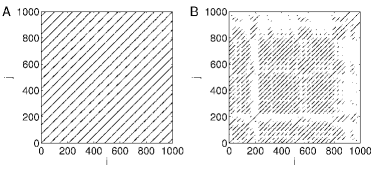
Figure 1: Recurrence plots for a periodic (A) and a chaotic (B) trajectory of the Rössler system (9) (see Sec. III.2 for details).

II.2 Quantitative analysis of recurrence networks

Recurrence networks (RNs) are spatial networks representing local neighborhood relationships in the phase space of a dynamical system. In a RN, every sampled point is represented by a vertex $v$, whereas edges indicate pairs of observations whose mutual distance in phase space is smaller than the pre-defined threshold $\varepsilon$. The resulting edge density $\rho$, i.e., the relative fraction of edges that are actually present in comparison to a fully connected network, is then given by $RR$ (see Eq. (3)). Hence, characterizing topological properties of RPs by sophisticated network-theoretic quantifiers allows retrieving additional information about higher-order phase space properties of the system Donner2009 . It has been shown that these measures are able to capture dynamical transitions in complex systems, such as in the logistic map with changing control parameter or a real-world paleoclimatic time series, demonstrating that network-theoretic features provide additional and complementary information when compared to traditional RQA measures Marwan2009 .

In this work, we particularly consider the global clustering coefficient $\mathcal{C}$ and the average path length $\mathcal{L}$ of a RN. The application of other measures (e.g., betweenness centrality) is straightforward, but we argue that the description of network topology by a scalar parameter instead of a distribution of vertex- or edge-based statistics might be more suitable for detecting and quantifying qualitative changes in the dynamics of a system. Moreover, one has to note that state-of-the-art numerical algorithms for computing other complex network measures often require considerably larger computational efforts than estimating traditional RQA measures.

The local clustering coefficient $\mathcal{C}_{v}$ characterizes the phase space geometry of an attractor in the $\varepsilon$-neighborhood of a vertex $v$. Specifically, $\mathcal{C}_{v}$ gives the probability that two randomly chosen neighbors of $v$ are also neighbors watts_nature_1998 , i.e.,

$$\mathcal{C}_{v}=\frac{2}{k_{v}(k_{v}-1)}N^{\Delta}_{v},$$ (6)

where $k_{v}$ is the degree centrality (i.e., the number of neighbors of $v$, which coincides with the local recurrence rate $RR_{v}$), and $N^{\Delta}_{v}$ is the total number of closed triangular subgraphs including $v$, which is normalized by the maximum possible value $k_{v}(k_{v}-1)/2$. For vertices of degree $k_{v}=0$ or $1$ (i.e., isolated or tree-like vertices, respectively), $\mathcal{C}_{v}=0$ by definition since such vertices cannot participate in triangles. Instead of studying $\mathcal{C}_{v}$ individually for all vertices of a RN, we consider its average value taken over all vertices of a network, the global clustering coefficient

$$\mathcal{C}=\frac{1}{N}\sum_{v=1}^{N}\mathcal{C}_{v},$$ (7)

as a global characteristic parameter of network topology.

The local clustering coefficient $\mathcal{C}_{v}$ is related to the effective dimensionality of the set of observations in the $\varepsilon$-neighborhood of a vertex $v$ Donner2009 . In particular, we find specific dependencies for both continuous and discrete dynamical systems:

1. For discrete systems, periodic orbits consist only of a finite set of points. This implies that for $\varepsilon\ll\Delta$ with $\Delta\geq\max_{i,j}d_{i,j}$ being the attractor diameter, the RN is decomposed into disjoint components with multiple vertices being located at the same point in phase space. As a consequence, the individual components are fully connected for all $\varepsilon>0$, which leads to $\mathcal{C}=1$. In contrast, for chaotic trajectories, sufficiently small $\varepsilon\ll\Delta$ results in $\mathcal{C}<1$ Donner2009 .

2. For a continuous system, it is a well-established fact that if a chaotic trajectory enters the neighborhood of an unstable periodic orbit (UPO), it stays within this neighborhood for a certain time Lathrop_pra_1989 . As a consequence, states accumulate along this UPO instead of homogeneously filling the phase space in the corresponding neighborhood (in particular if we consider UPOs of lower period). Since from the theory of spatial random graphs Dall2002 it is known that the average clustering coefficient increases with decreasing spatial dimension of the space in which a network is embedded, it follows that parts of a chaotic attractor that are close to (low-periodic) UPOs are characterized by higher values of $\mathcal{C}_{v}$ in the resulting RNs Donner2009 . Following a related argument, we expect that states on a periodic orbit of a continuous system are also characterized by high values of $\mathcal{C}_{v}$, which implies high $\mathcal{C}$. In general, however, for chaotic trajectories the filling of the phase space with observed states is more homogeneous than for periodic ones, which leads to a tendency towards lower values of $\mathcal{C}_{v}$ and, hence, $\mathcal{C}$.

A second global measure of network topology is the average path length. Since we consider RNs as undirected and unweighted, we define all edges to be of unit length in terms of graph (geodesic) distance. The graph distance between any two vertices of the network is defined as the length of the shortest path between them. Hence, the shortest path length $l_{i,j}$ in the RN gives the minimum number of edges that have to be passed on a graph between two vertices $i$ and $j$. Accordingly, $l_{i,j}$ is related to the phase space distance of the associated states, but not to the temporal evolution of the system (Fig. 2).

The average path length $\mathcal{L}$ is defined as the mean value of the shortest path lengths $l_{i,j}$ taken over all pairs of vertices $(i,j)$,

$$\mathcal{L}=\left<l_{i,j}\right>=\frac{2}{N(N-1)}\sum_{i<j}l_{i,j}.$$ (8)

For disconnected pairs of vertices, the shortest path length is set to zero by definition. Note that in most practical applications, this has no major impact on the corresponding statistics. The average path length is related to the average separation of states in phase space, which measures the size of the attractor in units of $\varepsilon$. Note that since metric distances in the phase space are conserved, this implies an approximately reciprocal relationship $\mathcal{L}\propto\varepsilon^{-1}$ Donner2009 , with the exception of periodic orbits of discrete maps (see the arguments given above).

For the behavior of the average path length $\mathcal{L}$, one has to carefully distinguish between continuous and discrete systems again:

1. For discrete systems, the structure of a periodic orbit in phase space implies $\mathcal{L}=1$ by definition for $\varepsilon\ll\Delta$ Marwan2009 . In turn, for chaotic trajectories, there is a continuum of possible values, so that $\mathcal{L}>1$ for $\varepsilon\ll\Delta$. Hence, the average path length of a periodic orbit is smaller than that of a chaotic one.

2. For continuous systems, however, a periodic trajectory has a completely different structure in phase space, which means that $\mathcal{L}$ is approximately determined by the curve length of the orbit in the phase space (Fig. 2A). In contrast, for chaotic trajectories, there are “short-cuts” that allow reaching one position in phase space from another with a lower number of steps than by following the trajectory Donner2009 (Fig. 2B). Consequently, for a comparable attractor diameter $\Delta$ and the same recurrence threshold $\varepsilon$, $\mathcal{L}$ can be expected to have lower values for chaotic orbits. Alternatively, it is desirable to fix $RR$ instead of $\varepsilon$ to obtain RNs with approximately the same numbers of edges. A detailed discussion on the advantages of this approach is presented in Sec. III.4. In this case, we note that the different geometric structure of the attractor in both the periodic and chaotic regime even enhances the effect of shortcuts, so that under general conditions, periodic orbits of continuous systems are characterized by larger $\mathcal{L}$ than chaotic ones.

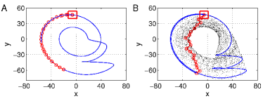
Figure 2: (Color online) Illustration of the shortest path length for two example trajectories of the Rössler system (9) in (A) periodic and (B) chaotic regime. The square is a schematic projection of the recurrence neighborhood to the $(x,y)$ plane. In these two particular examples, $l^{A}_{i,j}=24$ and $l^{B}_{i,j}=19$ for $\varepsilon=7.0$ (maximum norm).

Concerning the behavior of the average path length as shown in Fig. 2, we have to point out that differences between periodic and chaotic dynamics require that transient behavior (e.g., during some initial phase of the dynamics before the attractor has been reached by the considered trajectory) has been sufficiently removed, since such transients could also result in artificial short-cuts in phase space for periodic systems. While this problem can be easily solved in numerical studies by simply discarding the transients, it can contribute additional uncertainties in experimental studies where only a limited amount of data is available. In a similar way, using $\mathcal{L}$ for discriminating between periodic dynamics and chaos in noisy experimental time series is expected to lead to the same problem. However, in such cases, other network-theoretic quantities (e.g., $\mathcal{C}$) still provide feasible alternatives, to which the mentioned conceptual problem does not apply (at least for sufficiently small noise levels that do not exceed the order of magnitude of the recurrence threshold $\varepsilon$). In addition, there are other recurrence-based techniques such as recurrence time statistics, which allow distinguishing regular and chaotic dynamics even in challenging situations, e.g., quasi-periodicity versus weakly chaotic behavior Zou_quasiperiod ; Zou2007Chaos .

In summary, $\mathcal{C}$ shows a consistent behavior for discrete and continuous systems, whereas $\mathcal{L}$ performs inversely with respect to periodic and chaotic dynamics. This implies, that $\mathcal{L}$ cannot be used alone to classify the dynamics of time series from real systems, where the nature of the underlying process is unknown. Our results presented in this work and elsewhere Marwan2009 suggest, however, that $\mathcal{L}$ is nevertheless very well able to distinguish between periodic and chaotic behavior in the parameter space of the same dynamical system.

III Model: Chaotic Rössler system

III.1 Two-dimensional parameter space

As an illustrative example for a time-continuous dynamical system that shows shrimp structures in its parameter space, we study the Rössler system

$$\left(\frac{dx}{dt},\frac{dy}{dt},\frac{dz}{dt}\right)=\left(-y-z,x+ay,b+z(x-c)\right).$$ (9)

In this system, $c$ is often regarded as the standard bifurcation parameter, whereas $a$ and $b$ mainly change the shape of the attractor. In this work, however, we vary $a=b$ on the one hand, and $c$ on the other hand, which yields a two-dimensional parameter space of $(c,a)$. One of the parameter regions of special interest is $(c,a)\in[20,45]\times[0.2,0.3]$, where the chaotic regime is intermingled with periodic windows in a complex manner MTthesis . Thus, in the following, we pay special attention to this part of the parameter space. Note that shrimp structures are not confined to this particular plane in the three-dimensional parameter space of the Rössler system and, hence, investigating a differently oriented plane as in Bonatto2008PTRS would not qualitatively alter the results of our study.

For further analysis, the above mentioned part of the parameter space of $(c,a)$ is divided into $1,000\times 1,000$ grid points, which results in the step size $0.0001$ in $a\in[0.2,0.3]$ and $0.025$ in $c\in[20,45]$. We first consider the maximum Lyapunov exponent of the resulting systems as a characteristic measure to determine whether the trajectories resulting from each parameter combination are chaotic or periodic. For this purpose, all three Lyapunov exponents $\lambda_{i}$ have been computed based on Eq. (9) by numerically solving the associated variational equations Ott2002 . Numerical integration is carried out using a fourth-order Runge-Kutta integrator with a fixed step size of $h=0.001$ time units and randomly chosen initial conditions $(x_{0},y_{0},z_{0})\in[0,1]\times[0,1]\times[0,1]$. In order to provide sufficient data for an accurate estimation of Lyapunov exponents, the integration is performed for sufficiently long time (until $t=10,000$, i.e., involving $N=10,000,000$ data points with a sampling $\Delta t$ corresponding to the considered integration step $h$). For computing the different recurrence-based measures in a second step of analysis, the initial transients (cf. Sec. II.2) have been discarded by removing the first $500,000$ iterations (i.e., all data until $t=500$) from the simulated trajectories. Moreover, for all further calculations based on the recurrence matrices, a coarser sampling of $\Delta t=0.2$ (i.e., 200 integration steps) has been considered. For each trajectory, the sampling has been terminated after $N=5,000$ points (corresponding to about $150\sim 250$ oscillations of the system) have been obtained, yielding much shorter time series than those used for estimating Lyapunov exponents. Note that the specific choice of sampling time has a certain influence on the results discussed in the following. Specifically, the sampling corresponding to the optimum resolution of dynamically relevant features is expected to vary among different parameter settings. In this respect, the considered value of $\Delta t$ represents a reasonable and practically tractable choice.

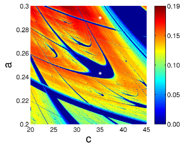
Figure 3: (Color online) Maximum Lyapunov exponent $\lambda_{1}$ in the $(c,a)$ parameter plane of the Rössler system (9). Regions with $\lambda_{1}=0$ indicate periodic dynamics, those with large $\lambda_{1}$ correspond to a strongly chaotic behavior. Asterisks indicate the parameter combinations used as examples in Sec. II and III.

The resulting maximum Lyapunov exponent $\lambda_{1}$ reveals a rich structure of chaotic and periodic dynamics in the parameter space (Fig. 3). Inside the chaotic regions, several well pronounced periodic bands are identified. Moreover, in the center of the plot, a special periodic window of interest is found, with structures resembling a head and four main thin legs. These particular swallow-like structures can be identified as shrimps MTthesis . Additional zooms into the parameter space uncover numerous fine structures, which correspond to secondary shrimps.

III.2 Prototypical trajectories

We first illustrate the potentials of recurrence-based approaches for discriminating between periodic and chaotic dynamics by studying trajectories obtained from two distinct parameter combinations. Based on the parameter space shown in Fig. 3, the dynamics is periodic for $(a,b,c)=(0.245,0.245,35)$, while chaotic for $(a,b,c)=(0.29,0.29,35)$. The Lyapunov exponents are $(0,-0.223,-32.683)$ for the periodic trajectory, and $(0.151,0,-32.517)$ for the chaotic one. The typical phase space distances of states on the two trajectories are of the same order of magnitude (Tab. 1), which is illustrated by the probability distribution of the mutual distances $d_{i,j}$ in Fig. 4A. However, the detailed relationship of $RR(\varepsilon)$ is clearly different: for a low (but fixed) $RR$, we have to consider much higher $\varepsilon$ for chaotic trajectories than for periodic ones, while for larger $RR(\varepsilon)$, the opposite behavior is found (Fig. 4B). $RR$ corresponds to the correlation sum, the slope of which in a double logarithmic plot gives the correlation dimension $D_{2}$. Therefore, $RR(\varepsilon)$ having a larger slope for the chaotic trajectory than for the periodic one (Fig. 4B) indicates that the correlation dimension of the former is higher than that of the latter.

	periodic	chaotic
$\lambda_{1}$	$0.0\pm 0.0003$	$0.15\pm 0.0002$
$\left<d_{i,j}\right>$	$58.95\pm 0.14$	$57.42\pm 3.03$
$\max_{i,j}d_{i,j}$	$476.69\pm 0.15$	$575.12\pm 23.99$
$\varepsilon\left(RR=0.02\right)$	$4.79\pm 0.14$	$6.50\pm 0.53$
$DET$	$0.99\pm 0.01$	$0.97\pm 0.01$
$L_{MEAN}$	$18.51\pm 0.18$	$10.60\pm 0.34$
$\mathcal{C}$	$0.77\pm 0.001$	$0.62\pm 0.004$
$\mathcal{L}$	$45.30\pm 1.83$	$9.19\pm 0.37$

Table 1: Maximum Lyapunov exponents $\lambda_{1}$ ($N=10,000,000$, $\Delta t=0.001$), mean and maximum separation of points in phase space ($N=5,000$, $\Delta t=0.2$) and resulting recurrence threshold $\varepsilon$ (maximum norm) for $RR=0.02$, and RQA ($l_{min}=2$) and network measures for two parameter combinations (see text), representing periodic and chaotic regimes of the Rössler system. The error bars correspond to the standard deviation obtained from $100$ realizations with different initial conditions. Note that the large variance of the metric quantities $\varepsilon$ and $d_{ij}$ for the chaotic trajectory is a common result when working with short time series and different initial conditions Donner2009b .

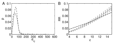
Figure 4: (A) Probability distributions $p(d_{i,j})$ of mutual distances $d_{i,j}$ (maximum norm) between states on one realization ($N=5,000$) of periodic (solid) and chaotic (dashed) trajectories, respectively (see text). (B) Dependence of the recurrence rate $RR$ on the recurrence threshold $\varepsilon$ for a periodic and chaotic regime. The error bars correspond to the standard deviation obtained from $100$ realizations with different initial conditions.

Both RQA and complex network measures highlight differences in the topological structure between the periodic and chaotic regimes (Tab. 1). We observe that for the considered recurrence rate ($RR=0.02$), $DET$, $L_{MEAN}$, $\mathcal{C}$ and $\mathcal{L}$ have lower values for chaotic trajectories than for periodic ones (which distinctively differs from the behavior of the maximum Lyapunov exponent $\lambda_{1}$), while the difference is significant for the latter three measures. However, before being able to generalize these findings, the robustness of the aforementioned features has to be critically examined. Our corresponding results are summarized in the following two subsections.

III.3 Dependence on $l_{min}$

For the computation of most line-based RQA measures (with some exceptions, such as $RR$ or the maximum diagonal line length), one has to choose a proper minimal line length $l_{min}$, to avoid a bias due to oversampling Marwan_report_2007 . The particular values of these measures do significantly depend on $l_{min}$ (Fig. 5), although the discrepancy between the values of $DET$ and $L_{MEAN}$ obtained for periodic and chaotic trajectories remains qualitatively unchanged (in general, the values of $DET$ and $L_{MEAN}$ are larger for a periodic trajectory than for a chaotic one). Note that $DET$ and $L_{MEAN}$ are more robust against noise than other measures like the maximum diagonal line length Marwan_report_2007 .

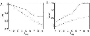
Figure 5: Dependence of the RQA measures $DET$ (A) and $L_{MEAN}$ (B) on $l_{min}$ for periodic (solid) and chaotic (dashed) trajectories. The error bars indicate the standard deviation obtained from $100$ realizations of the Rössler system (9) with $N=5,000$, $\Delta t=0.2$, $RR=0.02$, and different initial conditions.

III.4 Dependence on the recurrence threshold

Since all considered measures are based on the recurrence matrix, their values necessarily depend on the choice of the recurrence threshold $\varepsilon$. So far, there is no universal threshold selection criterion for the RP computation. On the one hand, if $\varepsilon$ is chosen too small, there are almost no recurrence points and, hence, no feasible information on the recurrence structure of the system. On the other hand, if $\varepsilon$ is too large, almost every point is a neighbor of every other point, which leads to numerous artifacts. Hence, we have to seek a compromise for choosing a reasonable value of $\varepsilon$. One rule of thumb is choosing $\varepsilon$ in such a way that it lies in the scaling regime of the double logarithmic plot of the correlation integral versus $\varepsilon$. This rule coincides with the classical strategy for estimating the correlation dimension $D_{2}$ using the Grassberger-Procaccia algorithm Grassberger_prl_1983 . Following independent arguments, Schinkel et al. Schinkel2008 suggested choosing $\varepsilon$ corresponding to at most $5\%$ of the maximum attractor diameter in phase space. In a similar way, $RR\lesssim 0.05$ has been found a reasonable choice in the analysis of RNs Marwan2009 ; Donner2009 ; Donner2009b .

The dependence of RQA and RN measures on $\varepsilon$ is shown in Fig. 6. One observes that all previously discussed measures are clearly able to distinguish between periodic and chaotic dynamics, i.e., they show significant differences in a broad interval of $\varepsilon$ (corresponding to mean recurrence rates of about 1% to 5%).

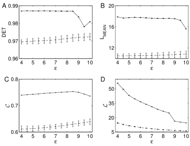
Figure 6: Dependence of the RQA measures $DET$ (A), $L_{MEAN}$ (B), and the network measures $\mathcal{C}$ (C) and $\mathcal{L}$ (D) on the recurrence threshold $\varepsilon$ for periodic (solid) and chaotic (dashed) trajectories (see text). The error bars indicate the standard deviation obtained from $100$ realizations of the Rössler system (9) with $N=5,000$, $\Delta t=0.2$, $l_{min}=2$, and different initial conditions.

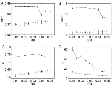
Figure 7: Same as in Fig. 6 for the dependence of these measures on the recurrence rate $RR$.

Instead of fixing the recurrence threshold $\varepsilon$, it may be desirable to compare different situations by using RPs with a fixed value of $RR$. Firstly, the resulting RNs have approximately the same number of edges, which allows comparing the resulting topological properties of different networks more objectively. Secondly, it has been shown in Fig. 4B that there is a crossover between the $RR$ of periodic and chaotic trajectories obtained with the same $\varepsilon$, which is related to the fact that $RR(\varepsilon)$ (which corresponds to the correlation sum) increases exponentially for a chaotic trajectory Grassberger_prl_1983 . Finally, we have to note that the amplitudes of the (chaotic or periodic) oscillations of the Rössler system change with the specifically chosen control parameters of the system. In order to automatize the numerical algorithms for estimating all RP-based measures, fixing $\varepsilon$ would lead to values of $RR$ and other RQA measures that cannot be compared in a meaningful way. A related approach using the dependence on $RR$ has already been applied for an automatized detection of the scaling region in the recurrence-based estimation of $K_{2}$ for the study of a large scale system Planetary .

According to the above arguments, we will use a fixed value of $RR$ in all following calculations. Because of this, in a first step of analysis, we study the dependence of the different measures on $RR$ in some detail similar to the dependence on $\varepsilon$ discussed above. Figure 7 reveals that the difference between periodic and chaotic orbits remains qualitatively unchanged and does not depend on the specific choice of $RR$. Specifically, in all four cases, periodic trajectories are characterized by larger values of the different measures.

IV Results

In the following, we study the performance of the different recurrence-based measures for identifying shrimp structures in the Rössler system. For this purpose, we take $\lambda_{1}$ as a reference, since this measure per definition discriminates between periodic ($\lambda_{1}=0$) and chaotic ($\lambda_{1}>0$) dynamics. Note that in order to reach reliable estimates of $\lambda_{1}$, typically a large amount of data is required. In contrast, recent results on RQA and RN measures Marwan2009 suggest that these methods allow identifying dynamical transitions in complex systems using much shorter time series.

In order to systematically test the applicability of recurrence-based methods for identifying shrimps, we use the same grid with $1,000\times 1,000$ pairs of points in the $(c,a)$-parameter plane as in Fig. 3. For each set of parameters, we consider time series of $N=5,000$ data points sampled with a fixed time step of $\Delta t=0.2$ for estimating all RQA and RN measures. Initial transients have been removed from the data as described in Sec. IIIA. We stress that measures originated from both RQA and network theory are computed from the same recurrence matrices $R_{i,j}$ (which have been constructed from the original three-dimensional coordinates of the system without embedding), so that the resulting structures in the parameter space are well comparable. In the following, we will consistently use $l_{min}=2$ and $RR=0.02$.

IV.1 Behavior of individual measures

The values of the four chosen measures in dependence on the parameters $a$ and $c$ are shown in Fig. 8. We find that all four measures are indeed able to identify periodic windows, in particular, those associated with shrimp structures. However, the discriminatory power of the individual parameters for distinguishing between periodic and chaotic regions is notably different. Specifically, for the chosen values of $l_{min}$ and $RR$ the contrast in the values of $DET$ obtained for both regimes is relatively weak (see Figs. 5 and 7 and Tab. 1), whereas the other three measures show a much larger range of values.

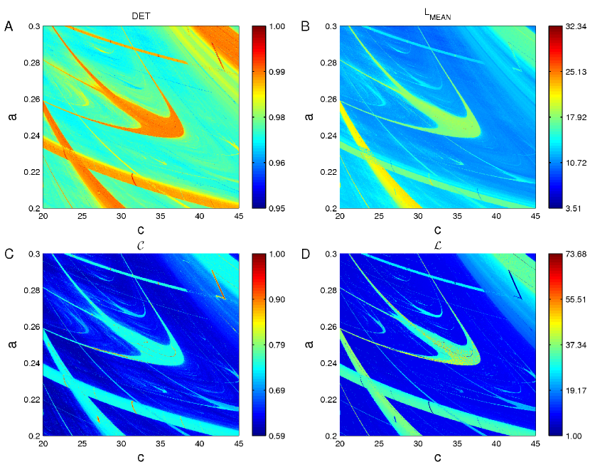
Figure 8: (Color online) RQA measures $DET$ (A), $L_{MEAN}$ (B), and network measures $\mathcal{C}$ (C) and $\mathcal{L}$ (D) in the $(c,a)$ parameter plane of the Rössler system (9).

Unlike $DET$ and $L_{MEAN}$, $\mathcal{C}$ and $\mathcal{L}$ resolve all periodic regimes including band structures and even secondary shrimps. The main remaining difference to the structures obtained by using the maximum Lyapunov exponent (Fig. 3) is found in the broad periodic band in the upper right corner of the parameter plane. In this region of parameter space, the system shows a complex bifurcation scenario, including different routes from periodic behavior to chaos similar to those associated with shrimp structures in other continuous dynamical systems Zou_ijbc_2005 . These differences are partially related to numerical inaccuracies in the presence of time series with a finite length and become less pronounced if longer simulations are used. Since no analytical solutions of the system are available for this specific region, additional application of complementary numerical methods (e.g., Lyapunov exponents, return maps, Poincaré sections, etc.) would be necessary for completely identifying the associated bifurcation scenario, which is however out of the scope of this paper.

IV.2 Correlations between recurrence-based measures and $\lambda_{1}$

We now perform a more detailed quantitative analysis of the power of the individual measures as discriminatory statistics between periodic and chaotic dynamics. For this purpose, the differences between the structures obtained using the discussed measures and those revealed by $\lambda_{1}$ can be interpreted as a lack of performance. Since the different measures are characterized by strongly differing probability distribution functions (PDFs), we seek a statistics that allows properly quantifying deviations between the respective structures in the parameter space. The first insight into this question is provided by the correlation coefficients between $\lambda_{1}$ and the other measures, which are in all cases clearly significant, but with a negative sign (Tab. 2). This result supports the findings in Sec. III for the two example trajectories.

In order to study how strongly the patterns of the different measures in the $(c,a)$-plane resemble those found for the maximum Lyapunov exponent, we investigate the point-wise difference of the corresponding cumulative distribution functions (CDFs), i.e.,

$$\Delta P(\lambda_{1},x)=P(\lambda_{1})-P(x),$$ (10)

where $P(x)$ is (for a given $(c,a)$-combination) the empirical value of the CDF of the measure $x$ obtained from all 1,000,000 parameter combinations. In order to simplify the notation, the arguments $(c,a)$ of $\Delta P(\lambda_{1},x)$ will be suppressed. Note that the maximum absolute value of $\Delta P$, commonly denoted $D$, corresponds to the Kolmogorov-Smirnov statistics frequently used for testing the homogeneity of the probability distributions of two samples James2006 . Since all four recurrence-based measures are negatively correlated with $\lambda_{1}$, we will identify $x$ with $1-DET$, $1-L_{MEAN}$, $1-\mathcal{C}$, and $1-\mathcal{L}$, respectively.

	$\rho$	$\sigma^{2}_{\Delta P}$
$DET$	-0.75	0.21
$L_{MEAN}$	-0.81	0.18
$\mathcal{C}$	-0.70	0.23
$\mathcal{L}$	-0.66	0.24

Table 2: Overall performance indicators obtained from a point-wise comparison of the values of the maximum Lyapunov exponent $\lambda_{1}$ and the different RQA and network measures: Spearman’s $\rho$ and the standard deviation $\sigma^{2}$ of the CDF differences $\Delta P(\lambda_{1},x)$. For simplicity, the arguments of the different characteristics have been omitted.

Due to the significant correlations between the different measures (Tab. 2), we expect that the CDF difference $\Delta P(\lambda_{1},x)$ is close to zero in large parts of the parameter space. The patterns of the CDF differences are shown in Fig. 9. In all cases, values close to zero can often be observed in periodic windows (although differences appear especially in the secondary shrimps), whereas the shortness of the considered time series leads to significant deviations from zero in the chaotic regions. The standard deviations $\sigma^{2}_{\Delta P}$ of the CDF field provide a rough impression of the amount of incorrectly identified regimes (partially due to the finite length of time series), which will be quantitatively characterized in the next section.

Figure 9: (Color online) CDF differences $\Delta P(\lambda_{1},\cdot)$ between the maximum Lyapunov exponent $\lambda_{1}$ and the RQA measures $DET$ (A), $L_{MEAN}$ (B), and network measures $\mathcal{C}$ (C) and $\mathcal{L}$ (D) in the $(c,a)$ parameter plane of the Rössler system (9).

IV.3 Probability of classification errors

The general treatment in Sec. IV.2 do not yet allow sophisticated conclusions on which particular measure is most appropriate for detecting shrimps in continuous systems. In order to assess the discriminatory power of all four measures in more detail, we subject the resulting patterns in parameter space (Fig. 8) to further statistical analysis. For this purpose, we explicitly make use of the fact that the $(c,a)$-parameter plane of the Rössler system is composed of two sets of parameter combinations belonging to trajectories with periodic and chaotic dynamics, respectively. However, the corresponding group structure is not exactly known, since there are numerous $(c,a)$-combinations which lead to small values of $\lambda_{1}$ (Fig. 10). These corresponding values could hence be related to either weakly chaotic behavior or periodic dynamics that cannot be exactly detected due to the numerical precision. Note that no fixed points ($\lambda_{1}<0$) are found in our parameter space. In order to obtain a robust approximation of the two distinct groups of parameter combinations leading to $\lambda_{1}=0$ and $\lambda_{1}>0$, respectively, we refer to a (variable) critical value $\lambda^{*}$ (Fig. 10) for defining two disjoint sets

$$S_{1}(\lambda^{*}) := \{(c,a)|\lambda_{1}(c,a)\leq\lambda^{*}\}$$

$$S_{2}(\lambda^{*}) := \{(c,a)|\lambda_{1}(c,a)>\lambda^{*}\}$$

with group sizes $n_{1}$ and $n_{2}=n-n_{1}$ ($n=1,000,000$ in our case).

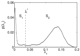
Figure 10: Probability distribution function of the maximum Lyapunov exponent $\lambda_{1}$ obtained from all 1,000,000 parameter combinations in the considered $(c,a)$ plane of the Rössler system (9).

IV.3.1 $F$ and $U$ tests

One possibility for assessing the discriminatory power of the different recurrence-based measures is taking the respective groups $S_{1}$ and $S_{2}$ (for different values of $\lambda^{*}$ in a reasonable range, i.e., $\lambda^{*}\in[0,0.05]$, see Fig. 10) and statistically quantifying whether or not main statistical characteristics of the distributions $p(x|S_{i})$ of the different measures $x$ obtained for both groups $S_{1}$ and $S_{2}$ differ significantly. For one specific choice of $\lambda^{*}$, these distributions are shown in Fig. 11. Formally, this question corresponds to a one-way analysis of variance (ANOVA) problem Montgomery2009 , with the factor being determined by two classes of values of $\lambda_{1}$. In order to evaluate whether the group means do significantly differ (in comparison with the respective group variances), the $F$-test is used with the test statistics Lomax2007

$$F=n_{1}n_{2}\frac{(\mu_{1}-\mu_{2})^{2}}{n_{1}s_{1}^{2}+n_{2}s_{2}^{2}}\equiv t^{2},$$ (11)

where $t$ is the test statistics of a corresponding $t$-test Welch1947 . Since we are aware that the values of $F$ (or, alternatively, $t$) may be misleading if the underlying sample PDFs are strongly non-Gaussian (see Fig. 11), our results are complemented by those of a corresponding distribution-free test. Specifically, we compute the value of the test statistics $U$ of the Mann-Whitney $U$-test Conover1999 ; Hollander1999 against equality of the medians of two distributions, which can be considered as the equivalent of an $F$-test performed on the sets of rank numbers.

Figure 11: PDFs $p(x|S_{i})$ of RQA and RN measures for parameter combinations $(c,a)$ yielding maximum Lyapunov exponents $\lambda_{1}<\lambda^{*}$ (S₁) and $\lambda_{1}>\lambda^{*}$ (S₂) with $\lambda^{*}=0.01$, respectively.

For both tests, we find that for almost all choices of $\lambda^{*}$, $\mathcal{L}$ and $\mathcal{C}$ show the highest values of the respective test statistics, indicating that the discriminatory power for distinguishing between both sets is the largest for these measures (Fig. 12A,B). Note that in all cases, the probability values for rejecting the respective null hypotheses (i.e., equality of group means and medians, respectively) are close to 100% due to the large sample size. The results obtained using both test statistics are supported by a numerical approximation of the associated overlap integral

$$\Psi=\int_{\min(x)}^{\max(x)}dx\ p(x|S_{1})\ p(x|S_{2})$$ (12)

of the PDFs of the recurrence based measures $x$ for both groups (Fig. 11), the values of which are shown in Fig. 12C.

The advantages of RN measures (at least for this particular case) become particularly apparent when visually inspecting Fig. 11. The overlap of the PDFs $p(x|S_{i})$ can be seen to be substantially smaller for the network quantifiers $\mathcal{C}$ and $\mathcal{L}$ (Fig. 11C,D), than for the RQA measures $DET$ and $L_{MEAN}$ (Fig. 11A,B).

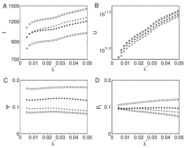
Figure 12: Measures for the discriminatory skills of the different recurrence-based measures $DET$ ($\bullet$), $L_{MEAN}$ ($\Box$), $\mathcal{C}$ ($+$), and $\mathcal{L}$ ($\triangleright$), obtained from a comparison with the results derived using the maximum Lyapunov exponent in dependence on the choice of $\lambda^{*}$: (A) $t$-test statistics, (B) $U$-test statistics, (C) overlap integral $\Psi$ (Eq. (12)), and (D) relative frequency of false detections $p_{f}$, using the same quantiles of $\lambda_{1}$ and the respective measures.

IV.3.2 Group overlap for fixed probability quantiles

In order to further study the differences in the performance of the considered measures, we apply another complimentary statistical test. Specifically, we take the $\alpha$-quantile $Q_{\alpha}(\lambda_{1})$ of the distribution of $\lambda_{1}$ that corresponds to a given value $\lambda^{*}$ (i.e., $\alpha\simeq n_{1}/n$) and consider a related decomposition of the $(c,a)$ parameter plane based on the same quantile for the recurrence-based measures, i.e.,

$$S^{\prime}_{1}(Q_{\alpha}(x)) := \{(c,a)|x(c,a)\leq Q_{\alpha}(x)\}$$

$$S^{\prime}_{2}(Q_{\alpha}(x)) := \{(c,a)|x(c,a)>Q_{\alpha}(x)\}$$

with $x\in\{1-DET,1-L_{MEAN},1-\mathcal{C},1-\mathcal{L}\}$. Since the quantile $\alpha$ has been kept fixed here, $S^{\prime}_{1}$ and $S^{\prime}_{2}$ contain the same numbers of elements ($n_{1}$ and $n_{2}$, respectively) as $S_{1}$ and $S_{2}$. Hence, we are able to quantitatively assess the coincidence between the grouping based on $\lambda_{1}$ and $x$ by considering the relative frequency $p_{f}$ of $(c,a)$ pairs that do not belong to the same group based on the two different measures. Figure 12D demonstrates that with respect to this criterion, the average path length $\mathcal{L}$ again shows (on average) the lowest frequency of “grouping errors” in comparison to $\lambda_{1}$, followed by $\mathcal{C}$, $DET$ and $L_{MEAN}$.

IV.3.3 ROC analysis

An even more detailed characterization of classification errors is obtained in terms of the receiver operating characteristics (ROC) Fawcett2006 . In the ROC analysis, we compare the discrimination ($S_{1}$, $S_{2}$) of the set of parameters $(c,a)$ based on a fixed value of $\lambda^{*}$ with another grouping ($S^{\prime}_{1}$, $S^{\prime}_{2}$) based on a variable threshold $x^{*}$ of the observable $x$, which now replaces the quantile $Q_{\alpha}(x)$. The probabilities of correct as well as false detections of periodic behavior, $p_{c}^{(p)}$ and $p_{f}^{(p)}$, respectively, are given as

$$p_{c}^{(p)}(\lambda^{*},x^{*}) = \left|S^{\prime}_{1}\cap S_{1}\right|/\left|S_{1}\right|$$

$$p_{f}^{(p)}(\lambda^{*},x^{*}) = \left|S^{\prime}_{1}\cap S_{2}\right|/\left|S_{2}\right|$$

where $\left|S\right|$ represents the cardinality (i.e., the number of elements) of the set $S$. Varying $x^{*}$ over the full range of possible values with $\lambda^{*}$ simultaneously being kept fixed, we obtain a continuous curve in the $(p_{f}^{(p)},p_{c}^{(p)})$-plane, the ROC curve, which illustrates the trade-off between a high probability of correct and a low probability of false detections of periodic behavior (Fig. 13A). The area under this curve, $AUC$, can be (among other statistics) used for quantitatively characterizing the classification performance of different measures Fawcett2006 (Fig. 13B). Specifically, high values of $AUC$ correspond to a low probability of false classifications (i.e., high specificity) and, simultaneously, a high probability of correct classifications (i.e., high sensitivity). In contrast to all other kinds of statistical tests, the ROC analysis suggests that in the specific setting studied in this work, among the four considered measures, $\mathcal{C}$ is the most suitable statistics for discriminating between periodic and chaotic behavior of the Rössler system, followed by $\mathcal{L}$, $DET$, and $L_{MEAN}$.

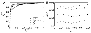
Figure 13: (A) ROC curves for $\lambda^{*}=0.01$, and (B) area under the ROC curve ($AUC$) in dependence on $\lambda^{*}$ for all four measures. For $\lambda^{*}=0.01$, $AUC$ takes the values $0.9279$ ($DET$), $0.9090$ ($L_{MEAN}$), $0.9487$ ($\mathcal{C}$), and $0.9442$ ($\mathcal{L}$), respectively.

One has to note that the overall classification error

$$\begin{split}p_{f}&=p_{f}^{(p)}(\lambda^{*},Q_{\alpha}(x))+p_{f}^{(c)}(\lambda^{*},Q_{\alpha}(x))\\ &=p_{f}^{(p)}(\lambda^{*},Q_{\alpha}(x))+\left(1-p_{c}^{(p)}(\lambda^{*},Q_{\alpha}(x))\right)\end{split}$$ (13)

(with $p_{f}^{(c)}(\lambda^{*},Q_{\alpha}(x))=|S^{\prime}_{2}\cap S_{1}|/|S_{1}|$ being the relative frequency of false detections of chaotic dynamics) still reaches values of around $10\%$ even for the best performing measures (Fig. 12D). The main reason for this performance failure is the different sensitivity of $\lambda_{1}$ and the recurrence-based measures close to the bifurcation lines (see Fig. 14). Apart from this, all four measures allow recovering the overall structures in parameter space comparably well as $\lambda_{1}$. The obvious differences in the transition regions could be related to the use of short time series in regions with a complex bifurcation scenario, which are probably affected by problematic features such as longer transients before the attractor is reached (see Sec. II.2), different bifurcation scenarios characterizing the transition between periodic and chaotic dynamics across different boundaries of the same shrimp, intermittency, or different stiffness properties of the considered trajectories Gallas1 ; Zou_ijbc_2005 .

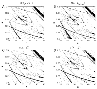
Figure 14: Discrimination errors (black dots) for the quantile-based groupings $S_{1}$, $S_{2}$, $S^{\prime}_{1}$, and $S^{\prime}_{2}$ for $\lambda^{*}=0.01$ (see Sect. IV.3.2) for (A) $DET$ ($p_{f}=0.0923$), (B) $L_{MEAN}$ ($0.1106$), (C) $\mathcal{C}$ ($0.0954$), and (D) $\mathcal{L}$ ($0.0899$).

V Conclusions

We have proposed to use nonlinear recurrence-based characteristics of time series for exploring the parameter space of complex systems. This is of special importance when dealing with experimental data. Specifically, for distinguishing periodic and chaotic dynamics, in the recent literature estimates of the maximum Lyapunov exponent $\lambda_{1}$ from the corresponding ODEs have most often been used, which allow resolving the borders of shrimps in a satisfactory way (see Fig. 3). This specific approach works well if the associated variational equations are provided explicitly. However, if these equations are not available (as in the case of experimental data), the numerical estimation of $\lambda_{1}$ is typically much more challenging, especially when dealing with short time series Kantz97 . The recurrence-based measures used in this work have the advantage that they can be properly estimated from rather short time series, so that they could prove advantageous also in situations where the available amount of data is not sufficient for obtaining reliable estimates of Lyapunov exponents. Using recurrence-based methods instead of Lyapunov exponents therefore has great potentials for the automatized discrimination between different types of dynamics in many applications. Specifically, the alternative discriminatory statistics introduced in this work could become very helpful not only in evaluating, but also already in designing both experimental and numerical studies, since the requirements concerning the necessary amount of data can be much easier matched. As a perspective, we therefore expect that systematic application of the proposed methods will open new fields of applications, as it has already been the case with the introduction of RQA Marwan_report_2007 . However, there are still situations where the consideration of Lyapunov exponents is clearly superior for detecting periodic windows in comparison to the recurrence-based approach, in particular when the governing equations are explicitly known or the available observations of the considered systems are very long. It will remain a subject of future studies to investigate in more detail under which specific conditions which of the two approaches is favorable.

Another traditional idea to distinguish periodic behavior from chaotic dynamics is to use a properly defined surface in phase space for a Poincaré section, since a periodic trajectory has only a finite number of intersection points with this surface, while a chaotic one renders an infinite number of crossings. Note, however, that constructing a proper Poincaré section for a given set of ODEs HenonP_phyD_1982 is much easier than it is the case when working with time series, where one most often relies on some interpolation techniques to find crossings on the section, which obviously introduces noise-like effects Kantz97 . Furthermore, there are no universal criteria for choosing Poincaré sections when scanning a large parameter space (e.g., Fig. 3) since the shape and the orientation of the attractors typically vary for different parameter values.

In this work, we have been particularly interested in the problem of detecting specific periodic windows in parameter space, so-called shrimps, which are characterized by a rich bifurcation scenario and self-similarity. Specifically, we have addressed the problem of numerically detecting shrimps in systems of ODEs, while the related question of the associated bifurcation scenarios remains a subject for future investigations. We expect the recurrence-based methods proposed in this work to be particularly useful for this problem, especially concerning the properties of secondary shrimps and the quantitative analysis of possible transient behavior.

For properly identifying shrimps in parameter space based on recurrence plots, both measures from RQA and complex network theory have been applied. For the $(c,a)$ parameter plane of the Rössler system, especially the recently proposed application of network measures to the recurrence matrix of complex systems Marwan2009 ; Donner2009 yields results coinciding well with those obtained using $\lambda_{1}$. The used RQA measures in this paper need two parameters recurrence rate $RR$ and minimum line length $l_{min}$, RN measures depend exclusively on $RR$. We have to emphasize that this conceptual advantage comes at the cost of higher computational demands, especially when considering the average path length $\mathcal{L}$ of the RNs. However, the clustering coefficient $\mathcal{C}$, which has been found to perform best in our example when considering the most sophisticated statistical evaluation (ROC analysis), can be calculated at significantly lower costs. Generally, $\mathcal{C}$ seems to be very well suited for distinguishing periodic from chaotic dynamics, even for time series sampled at a very high rate, such as the examples presented in this work. However, for high sampling rates, $DET$ and $L_{MEAN}$ can have a reduced discriminatory performance since the typical line structures become too similar Marwan2011 . We additionally note that both network measures have shown a slightly better discriminatory power for secondary shrimps than the two RQA measures $DET$ and $L_{MEAN}$, at least for the specific setting used in this study. As we have not explicitly shown here, even larger performance errors can be observed for other line-based RQA measures. A more detailed investigation of possible impacts of other choices of $l_{min}$ and $RR$ has not yet been systematically performed, but will be subject of future studies. As a preliminary result, repeating all presented calculations with a different value of $RR=0.01$ supports all results discussed in detail for $RR=0.02$ in this paper.

The two specific network-theoretic quantities considered here have already been shown to be able to detect dynamical transitions in both model systems and real-world time series Marwan2009 . We note, however, that since both measures are invariant under permutations of the time coordinate Donner2009 , they exclusively capture the geometry of states associated to a specific trajectory in phase space. This is a distinctive difference to most existing methods of time series analysis, which are related to the study of temporal correlations. We hypothesize that the good performance of network measures in detecting shrimps could be related to this fact, since network measures take only information about spatial correlations (i.e., neighborhood relationships in phase space) into account.

While a rigorous theory interrelating the phase space properties captured by RN measures to traditional dynamical invariants is still missing, the algorithm for estimating the correlation entropy $K_{2}$ from RPs (which has also been successfully applied for detecting shrimps in continuous systems MTthesis ) has been justified theoretically fluid . Since the estimation of $K_{2}$, however, involves several steps MTthesis with some subjective issues (in particular, the choice of the scaling region for convergence), its computational demands are significantly higher than those of the complex network as well as RQA measures applied in this work. Particularly, a large range of values of $RR$ ($1\%\sim 99\%$) is often considered to yield a well defined plateau of $K_{2}(RR)$, while the method proposed in this paper works with just one chosen value of $RR$, dramatically reducing computational costs. Systematically calculating RN statistics as well as RQA measures can be easily automatized using a fixed recurrence rate $RR$, ideally with $RR\lesssim 0.05$ Schinkel2008 ; Donner2009b . Hence, we conclude that our approach allows a systematic numerical discrimination between periodic and chaotic dynamics of a continuous system, which is more practicable than other possible techniques especially when systematically studying higher-dimensional parameter spaces.

In relation with the problem of discriminating between two qualitatively different types of dynamics in a binary way, which has been discussed in this work, Lyapunov exponents have also found wide use in quantitatively characterizing the “chaoticity” of complex dynamics. Following the results from Tab. 2, we emphasize that the recurrence-based characteristics considered in this work may be used for similar purposes. In contrast to the discriminatory power, our corresponding initial results suggest that the applied RQA measures may be somewhat better suited for this purpose than the network-based concepts. However, further detailed statistical analysis is necessary in order to provide further evidence that this result holds in general. A detailed treatment of this question therefore remains subject of future studies.

- (1) J. Guckenheimer and P. Holmes, Nonlinear Oscillations, Dynamical Systems, and Bifurcations of Vector Fields (Springer, New York, 1990), 3rd ed.
- (2) Y. A. Kuznetsov, Elements of applied bifurcation analysis (Springer, New York, 2004), 3rd ed.
- (3) J. A. C. Gallas, Phys. Rev. Lett. 70, 2714 (1993).
- (4) J. A. C. Gallas, Physica A 202, 196 (1994).
- (5) C. Bonatto, J. Garreau, and J. A. C. Gallas, Phys. Rev. Lett. 95, 143905 (2005).
- (6) Y. Zou, M. Thiel, M. Romano, Q. Bi, and J. Kurths, Int. J. Bifurcation Chaos 16, 3567 (2006).
- (7) E. Barreto, B. Hunt, C. Grebogi, and J. Yorke, Phys. Rev. Lett. 78, 4561 (1997).
- (8) E. N. Lorenz, Physica D 237, 1689 (2008).
- (9) L. C. Martins and J. A. C. Gallas, Int. J. Bifurcation Chaos 18, 1705 (2008).
- (10) R. Perez and L. Glass, Phys. Lett. A 90, 441 (1982).
- (11) J. Belair and L. Glass, Phys. Lett. A 96, 113 (1983).
- (12) P. Gaspard, R. Kapral, G. Nicolis, J. Stat. Phys. 35, 697 (1984).
- (13) J. Bélair and L. Glass, Physica D 16, 143 (1985).
- (14) M. S. Baptista, Ph.D. thesis, University of São Paulo (1996).
- (15) M. Thiel, Ph.D. thesis, University of Potsdam (2004).
- (16) C. Bonatto and J. A. C. Gallas, Phil. Trans. Roy. Soc. A 366, 505 (2008).
- (17) J. A. C. Gallas, Int. J. Bifurcation Chaos 20, 197 (2010).
- (18) L. Glass, Nature 410, 277 (2001).
- (19) C. Bonatto and J. A. C. Gallas, Phys. Rev. E 75, 055204 (2007).
- (20) C. Bonatto and J. A. C. Gallas, Phys. Rev. Lett. 101, 054101 (2008).
- (21) V. Kovanis, A. Gavrielides, and J. A. C. Gallas, Eur. Phys. J. D 58, 181 (2010).
- (22) C. Bonatto, J. A. C. Gallas, and Y. Ueda, Phys. Rev. E 77, 026217 (2008).
- (23) H. A. Albuquerque, R. M. Rubinger, and P. C. Rech, Phys. Lett. A 372, 4793 (2008).
- (24) H. A. Albuquerque and P. C. Rech, Int. J. Bifurcation Chaos 19, 1351 (2009).
- (25) J. C. D. Cardoso, H. A. Albuquerque, and R. M. Rubinger, Phys. Lett. A 373, 2050 (2009).
- (26) E. R. Viana, R. M. Rubinger, H. A. Albuquerque, A. G. Oliveira, and G. M. Ribeiro, Chaos 20, 023110 (2010).
- (27) J. G. Freire, R. J. Field, and J. A. C. Gallas, J. Chem. Phys. 131, 044105 (2009).
- (28) S. L. T. de Souza, I. L. Caldas, and R. L. Viana, Math. Prob. Engin. 2009, 290356 (2009).
- (29) M. S. Baptista, M. B. Reyes, J. C. Sartorelli, C. Grebogi, and E. Jr. Rosa, Int. J. Bifurcation Chaos 13, 2551 (2003).
- (30) D. M. Maranho, M. S. Baptista, J. C. Sartorelli, and I. L. Caldas, Phys. Rev. E 77, 037202 (2008).
- (31) R. Stoop, P. Benner, and Y. Uwate, Phys. Rev. Lett. 105, 074102 (2010).
- (32) H. Kantz and T. Schreiber, Nonlinear Time Series Analysis (Cambridge University Press, Cambridge, 2004), 2nd ed.
- (33) J.-P. Eckmann, S. Kamphorst, and D. Ruelle, Europhys. Lett. 4, 973 (1987).
- (34) N. Marwan, M. Romano, M. Thiel, and J. Kurths, Phys. Rep. 438, 237 (2007).
- (35) M. Thiel, M. Romano, P. Read, and J. Kurths, Chaos 14, 234 (2004).
- (36) N. Marwan, J. F. Donges, Y. Zou, R. V. Donner, and J. Kurths, Phys. Lett. A 373, 4246 (2009).
- (37) J. Zhang and M. Small, Phys. Rev. Lett. 96, 238701 (2006).
- (38) X. Xu, J. Zhang, and M. Small, Proc. Natl. Acad. Sci. USA 105, 19601 (2008).
- (39) R. V. Donner, Y. Zou, J. F. Donges, N. Marwan, and J. Kurths, New J. Phys. 12, 033025 (2010).
- (40) R. V. Donner, M. Small, J. F. Donges, N. Marwan, Y. Zou, R. Xiang, and J. Kurths, Int. J. Bifurcation Chaos (in press).
- (41) J. Zbilut and C. Webber, Phys. Lett. A 171, 199 (1992).
- (42) L. Trulla, A. Giuliani, J. Zbilut, and C. Webber, Phys. Lett. A 223, 255 (1996).
- (43) N. Marwan, Eur. Phys. J. Special Topics 164, 3 (2008).
- (44) C. Webber, N. Marwan, A. Facchini, and A. Giuliani, Phys. Lett. A 373, 3753 (2009).
- (45) Y. Zou, D. Pazó, M. Romano, M. Thiel, and J. Kurths, Phys. Rev. E 76, 016210 (2007).
- (46) E. Ngamga, A. Nandi, R. Ramaswamy, M. Romano, M. Thiel, and J. Kurths, Phys. Rev. E 75, 36222 (2007).
- (47) E. Ngamga, A. Buscarino, M. Frasca, L. Fortuna, A. Prasad, and J. Kurths, Chaos 18, 013128 (2008).
- (48) D. J. Watts and S. H. Strogatz, Nature 393, 440 (1998).
- (49) D. Lathrop and E. Kostelich, Phys. Rev. A 40, 4028 (1989).
- (50) J. Dall and M. Christensen, Phys. Rev. E 66, 016121 (2002).
- (51) Y. Zou, M. Thiel, M.C. Romano, and J. Kurths, Chaos 17, 043101 (2007).
- (52) E. Ott, Chaos in dynamical systems (Cambridge University Press, 2002), 2nd ed.
- (53) R. V. Donner, Y. Zou, J. F. Donges, N. Marwan, and J. Kurths, Phys. Rev. E 81, 015101(R) (2010).
- (54) P. Grassberger and I. Procaccia, Phys. Rev. Lett. 50, 346 (1983).
- (55) S. Schinkel, O. Dimigen, and N. Marwan, Eur. Phys. J. ST 164, 45 (2008).
- (56) N. Asghari, C. Broeg, L. Carone, R. Casas-Miranda, J. C. C. Palacio, I. Csillik, R. Dvorak, F. Freistetter, G. Hadjivantsides, H. Hussmann, et al., Astron. Astrophys. 426, 353 (2004).
- (57) F. James, Statistical Methods in Experimental Physics (World Scientific, Singapore, 2006), 2nd ed.
- (58) D. C. Montgomery, Design and Analysis of Experiments (Wiley, New York, 2009), 7th ed.
- (59) R. G. Lomax, Statistical Concepts: A Second Course for Education and the Behavioral Sciences (Lawrence Erlbaum Associates Inc., Mahwah, NJ, 2007).
- (60) B. Welch, Biometrika 34, 28 (1947).
- (61) W. J. Conover, Practical Nonparametric Statistics (Wiley, New York, 1999).
- (62) M. Hollander and D. A. Wolfe, Nonparametric Statistical Methods (Wiley, New York, 1999), 2nd ed.
- (63) T. Fawcett, Pattern Recogn. Lett. 27, 861 (2006).
- (64) M. Hénon, Physica D 5, 412 (1982).
- (65) N. Marwan, arXiv: 1007.2215 (2010).
- (66) G. Csárdi and T. Nepusz, InterJournal CX.18, 1695 (2006).