MARVELS-1b: A Short-Period, Brown Dwarf Desert Candidate from the SDSS-III MARVELS Planet Search

Abstract

We present a new short-period brown dwarf candidate around the star TYC 1240-00945-1. This candidate was discovered in the first year of the Multi-object APO Radial Velocity Exoplanets Large-area Survey (MARVELS), which is part of the third phase of the Sloan Digital Sky Survey (SDSS-III), and we designate the brown dwarf as MARVELS-1b. MARVELS uses the technique of dispersed fixed-delay interferometery to simultaneously obtain radial velocity measurements for 60 objects per field using a single, custom-built instrument that is fiber fed from the SDSS 2.5-m telescope. From our 20 radial velocity measurements spread over a $\sim\!370$ d time baseline, we derive a Keplerian orbital fit with semi-amplitude $K=2.533\pm 0.025$ km s^-1, period $P=5.8953\pm 0.0004$ d, and eccentricity consistent with circular. Independent follow-up radial velocity data confirm the orbit. Adopting a mass of $1.37\pm 0.11\,M_{\odot}$ for the slightly evolved F9 host star, we infer that the companion has a minimum mass of $28.0\pm 1.5\,M_{Jup}$, a semimajor axis $0.071\pm 0.002$ AU assuming an edge-on orbit, and is probably tidally synchronized. We find no evidence for coherent instrinsic variability of the host star at the period of the companion at levels greater than a few millimagnitudes. The companion has an a priori transit probability of $\sim\!14\%$. Although we find no evidence for transits, we cannot definitively rule them out for companion radii $\lesssim\!1\,R_{Jup}$.

1 INTRODUCTION

One of the first results to emerge from high-precision radial velocity (RV) surveys seeking substellar companions was the existence of a brown dwarf (BD) desert: a paucity of close ($a\lesssim\!5$ AU) brown dwarf ($13\,M_{Jup}\!\lesssim\!M\lesssim 80\,M_{Jup}$) companions to solar-type stars, relative to more common stellar mass companions (Marcy & Butler, 2000). Indeed, since they induce reflex radial velocity semiamplitudes of many hundreds of meters per second, such brown dwarf companions have been within the detection capabilities of these surveys for over two decades (e.g., Campbell et al. 1988), yet to date only a few dozen are known (Reid & Metchev 2008). On the other hand, as instrumentation has subsequently improved, first Jovian, and now terrestrial planetary companions in similar orbits have been found in relative abundance (Cumming et al., 2008; Mayor & Udry, 2008; Mayor et al., 2009). The brown dwarf mass regime represents an apparent minimum in the mass distribution of close companions to solar-type stars.

Planetary companions are believed to form in circumstellar protoplanetary disks, whereas stellar companions are believed to form by concurrent collapse or fragmentation, so the brown dwarf desert is commonly interpreted as the gap between the largest mass objects that can be formed in disks, and the smallest mass clump that can collapse and/or fragment in the vicinity of a protostar. Such a gap was by no means guaranteed to exist, and is perhaps surprising. For example, numerous isolated BDs in star-forming regions have been found to possess protoplanetary disks, akin to the disks of young stars, suggesting that BDs form much as stars do (e.g., Caballero et al., 2007; Luhman & Muench, 2008; Scholz & Jayawardhana, 2008). More generally, the mass function of isolated substellar objects in the field and clusters appears to be roughly flat in $\log{M}$ for masses down to at least $\sim\!20\,M_{Jup}$ (Luhman et al., 2000; Chabrier, 2002), whereas it is not clear what sets the upper limit for objects formed in protoplanetary disks (e.g., Boss, 2001; Ida & Lin, 2004; Rafikov, 2005; Dodson-Robinson et al., 2009; Kratter et al., 2010).

As such, details of the demographics of companions in the brown dwarf desert, including the aridity of the desert, the shape of the high-mass tail of the planetary companion mass function and the low-mass tail of the stellar companion mass function, as well as how these properties change with semimajor axis and primary mass, encode a wealth of information about the poorly understood physics of star and planet formation. Additional processes such as tidal evolution and disk-planet migration can also affect these properties (e.g., Armitage & Bonnell, 2002; Matzner & Levin, 2005), thus can be investigated via brown dwarf desert statistics.

Unfortunately, despite its potential diagnostic power, and after more than twenty years of precision radial velocity surveys, very little is known about the brown dwarf desert, precisely because brown dwarf companions are rare and so few such companions are known. The California & Carnegie Planet Search finds an occurrence rate of 0.7% $\pm$ 0.2% from their sample of $\sim\!1000$ target stars (Vogt et al. 2002, Patel et al. 2007), and the McDonald Observatory Planet Search agrees, with a rate of 0.8% $\pm$ 0.6% from a search sample of 250 stars (Wittenmyer et al., 2009). Gizis et al. (2001) suggest that brown dwarfs might not be as rare at wide separations (see also Metchev & Hillenbrand, 2004), although McCarthy & Zuckerman (2004) find a low rate of occurrence that is similar to that found for close separations. By extrapolating the mass functions of planets (on the low mass side) and stellar companions (on the high mass side) into the brown dwarf mass regime, Grether & Lineweaver (2006) find a mass of minimum occurrence (the driest part of the brown dwarf desert) at $31^{+25}_{-18}\,M_{Jup}$. They further suggest that the location of this minimum may scale with host star mass. For instance, the only known BD eclipsing binary is a “desert dweller”, consisting of a $\sim\!60\,M_{Jup}$ BD with a $\sim\!35\,M_{Jup}$ BD companion at a separation of $0.04$ AU (Stassun et al., 2006, 2007).

To make further progress on understanding the properties of the brown dwarf desert, a much larger sample of brown dwarf companions is needed. Furthermore, this larger sample must be drawn from a relatively uniform survey with a well-defined and homogeneous sample of primary target stars, so that the demographic properties of these companions can be reliably inferred. Given the occurrence rate of $\sim\!1\%$, a survey of $\sim\!10000$ stars is needed to detect of order 100 brown dwarf companions. Such an extensive survey would require a prohibitive amount of observing time with traditional echelle-based precision RV instruments, which can only target one object at a time. Furthermore, in many cases the RV precisions that can be achieved with these instruments are far better than are needed to detect brown dwarf companions, implying that this is not the most efficient application of these instruments.

The Multi-object APO Radial Velocity Exoplanets Large-area Survey (MARVELS; Ge et al., 2008) is a radial velocity survey of $\sim\!11000$ stars ($\sim\!10000$ dwarfs and subgiants, plus $\sim\!1000$ giants) with $7.6\!<\!V\!<\!12$ over time baselines of $\sim\!1.5$ years, with a stated goal of $<\!30$ m s^-1 precision for the faintest stars. It operates as one of the bright-time survey components of the Sloan Digital Sky Survey (SDSS) III, following on the legacy of the original SDSS (York et al., 2000). MARVELS uses the innovative instrumental technique of a dispersed fixed-delay interferometer (DFDI; see, e.g., Erskine & Ge, 2000; Ge, 2002; Ge et al., 2002; van Eyken et al., 2010) in order to simultaneously observe 60 objects at a time over a three degree field of view with a single instrument that is fiber fed from the SDSS 2.5-m Telescope (Gunn et al., 2006) at Apache Point Observatory. The fibers are fed through an interferometer, and both interferometer output beams are sent through a spectrograph with a resolving power $R\!\sim\!12000$, producing fringing spectra over the wavelength range $\sim\!500-570$ nm. Radial velocity information is imprinted in the phases of the fringes perpendicular to the dispersion axis of the spectrum due to a fixed variation in the interferometer delay along this direction.

By virtue of the large number of target stars, as well as uniform selection criteria described below, MARVELS is well suited to probe for rare companions. MARVELS commenced operations with SDSS-III in Sep. 2008, and as of the end of the first year’s data collection in Aug. 2009, had observed 780 stars with RV time series of more than 15 points. In this paper, we report the first MARVELS brown dwarf candidate, which we designate MARVELS-1b, detected in orbit around the star TYC 1240-00945-1 (Tycho-2 star catalogue; Høg et al. 2000).

2 OVERVIEW OF SDSS-III MARVELS TARGET SELECTION

The overall scope of MARVELS will be described in detail in future papers; we present a brief outline here in order to provide the context for the field and target selection of the brown dwarf candidate. MARVELS has been designed with an RV precision goal of $<\!30$ m s^-1 in order to be able to discover a sample of $\sim\!150$ new exoplanets, within a homogeneous parent sample of searched stars. By choosing a sample of target stars using a limited number of well-defined selection criteria, our sample suffers from minimal and well-understood biases, and can increase the size of the largest statistically homogeneous exoplanet sample by a factor of a few over that currently available.

MARVELS will run for six years during SDSS-III bright time, in a series of three cycles of self-contained two-year surveys. Each cycle will have a similar stellar target selection strategy, designed to give good survey coverage of FGK dwarfs and similar parent samples in each two-year cycle, although with different target fields. While in general this means only companions with up to $\sim\!1.5$ year periods will be detected, the advantage of this strategy is that we need not wait the full six years to gather enough epochs per star to detect companions. Also, this approach provides the opportunity to do major instrument upgrades at the end of each two-year cycle, without destroying the continuity of our RV measurements.

In order to collect enough photons to achieve $<\!30$ m s^-1 statistical RV precision, the stars we monitor must in general be brighter than $V\!\sim\!12$, although the precision at a given magnitude depends somewhat on stellar parameters as well. For the 60 object multiplexing capability of the instrument during the first two years (Sep. 2008–Sep. 2010), we found most fields on the sky were sufficiently rich to fill all the object fibers, so half of our fields were selected to include a reference star of $8\!<\!V\!<\!12$ with a known RV signal (stable or planet-hosting). By recovering the RV of the reference star, we can verify that the instrument is sufficiently stable to detect planetary companions. To ensure survey observability across all right ascensions, the remaining fields were selected from areas with no reference stars. Finally, we also selected some fields in the Kepler survey footprint (Borucki et al., 1997) in order to have the potential to leverage the exquisite Kepler photometry for any stars targeted by both surveys.

In each individual field, we used the intersection of the GSC2.3 (Spagna et al., 2006) and 2MASS (Skrutskie et al., 2006) catalogs as our initial targets database, but because many of our fields are in the Galactic plane and contaminated by giants, we conducted a preselection program to identify and reject giants from the sample prior to beginning RV monitoring. First, we performed a rough cut in magnitude and color, accepting only stars with $9.0\!<\!V\!<\!13.0$ and $(J-K)\!>\!0.29$. The faint magnitude limit rejects stars too faint for the survey, and the bright magnitude limit keeps the dynamic range small enough to avoid saturating the preselection observations. The color cut eliminates most hot stars from consideration, since we cannot obtain sufficient RV precision to detect planetary companions on any star hotter than mid-F. Second, we took spectral classification snapshots of the potential target stars using the SDSS double spectrographs (Uomoto et al., 1999) mounted on the SDSS 2.5-m Telescope, which have $R\!\sim\!1800$ and cover the wavelength range $390\!<\!\lambda\!<\!910$ nm.

The preselection observations were processed using the SDSS two-dimensional and one-dimensional spectroscopic pipelines (Stoughton et al., 2002). The spectroscopic parameters $T_{\rm eff}$, $\log g$, and [Fe/H] were derived using the SEGUE Stellar Parameter Pipeline (SSPP; Lee et al. 2008). Each spectrum was manually inspected to validate the parameters and to identify obvious binaries and emission line objects.

The final 60 targets for each field were selected using the following method. First, we only consider stars with $T_{\rm eff}<6250$ K. We dedicated 6 of the targets for observing giants, and identified the brightest available dwarfs and subgiants from $7.6\!<\!V\!<\!13.0$ to fill the other 54 targets, where dwarfs and subgiants are defined as having $\log{g}\!>\!3.0$. For $7.6\!<\!V\!<\!9.0$, we selected the targets for observation by conducting a literature search to reject known variable stars, and used a reduced proper motion (RPM) diagram to classify them as giants or dwarfs. While we prefer to pick bright dwarfs, in practice this bright magnitude range is dominated by giants, and therefore the MARVELS giant sample is typically drawn from the bright magnitude bin. For $9.0\!<\!V\!<\!13.0$, we ranked the stars by $V$ magnitude then picked the $\sim\!54$ highest-ranked stars, although to avoid the survey being dominated by F-stars, we cap the number of stars with $5800$ K$\!<\!T_{\rm eff}\!<\!6250$ K at no more than 24 out of 60. In practice, this combination of criteria usually completes our 60 target selection without going fainter than $V\!\sim\!11.5-12.0$. We do not impose selections based on the ages, activity levels, or metallicities of the stars.

We have recently learned that the original version of the SSPP code that we used for our target selection tends to overestimate $\log g$, particularly for cool temperatures of $T_{\rm eff}\!\lesssim\!5000$ K. While we are working on improved methods to better discriminate between dwarfs and giants for targeting in future survey cycles, our target sample for the first two year survey cycle is likely to have more giants than we desired; we estimate that up to 30% of targets in this sample could be giants due to the bias in the SSPP results. Note that we do not use the primary properties of TYC 1240-00945-1 derived from the SSPP in our subsequent analysis; we rely on the more accurate determinations from the detailed analysis of high-resolution spectra as described in §6. We only describe the SSPP target selection method here because our MARVELS targets for years 1 and 2 (including TYC 1240-00945-1) have been selected based on the SSPP results.

3 OBSERVATIONS AND PROCESSING

3.1 Primary Survey Observations with SDSS

TYC 1240-00945-1 was part of the first two-year cycle of the SDSS-III MARVELS planet search program described above. This target was selected for radial velocity monitoring using the preselection methodology and instrumentation described in §2. In preselection observations for this star’s field taken on Sep. 19, 2008, we obtained a series of five 7 s and five 12 s exposures of the target field, plus flat and arc lamp calibration exposures before and after this series. From preselection, the star appeared to be a late F-dwarf (but see further details in §6, which suggest it is starting to evolve into a subgiant) suitable for inclusion in the MARVELS RV monitoring.

Our discovery radial velocity observations were taken using the SDSS 2.5-m Telescope at Apache Point Observatory coupled to the MARVELS instrument, a 60 object fiber-fed DFDI (Ge et al., 2009). Our two-output interferometer produces two fringing spectra (“beams”) per object, over wavelengths $\sim\!500-570$ nm, with resolving power $R\!\sim\!12000$. The instrument is environmentally stabilized such that no iodine cell is needed in the stellar beam path, and instrument drift calibrations are simply taken before and after each stellar exposure. TYC 1240-00945-1 was observed at 20 epochs from Nov. 7, 2008 to Nov. 11, 2009, as listed in Table 1. Exposures were 50 min., yielding an average of 500 photons per CCD pixel on each $4\rm{k}\times 20$ pixel fringing spectrum. The RV signal on TYC 1240-00945-1 was easily detected by eye in the RV curves from the first year of MARVELS.

MARVELS RVs are differential measurements, based on the shift of the fringing spectrum relative to a template epoch. The RVs were derived from our 20 fringing spectrum observations using the preliminary version of our MARVELS DFDI pipeline, which is based on software from earlier DFDI prototype instruments (e.g., Ge et al. 2006). We provide here a brief outline of the mechanics of the MARVELS-specific pipeline, but leave a full description to future techniques papers to be written on the overall performance of the MARVELS hardware and survey.

After performing standard multi-object spectroscopic preprocessing on each frame such as bias subtraction, flatfielding, and trimming out individual spectra, we proceed to straighten slanted spectral lines, straighten tilted traces, and divide out uneven slit illumination to produce clean images ready for analysis. To remove a faint pattern of background fringes caused by the interferometer, we apply a low-pass filter, which leaves the fringes on stellar lines visible. The pipeline seeks to measure the epoch-to-epoch shift in the two-dimensional fringing spectrum (i.e., a spectrum with sinusoidal modulations along the slit direction). The shift induced by a stellar radial velocity change comprises two orthogonal components. The first component, a small shift of the stellar absorption lines along the wavelength axis, is the shift that conventional Doppler planet search instrumentation seeks to measure. The second component, a shift of the fringes on each absorption line along the spectrograph slit axis, is linearly proportional to the shift in the wavelength axis, but is amplified to a factor of a few times larger, and therefore provides most of the statistical leverage in our velocity measurement. At any given wavelength, the fringe shift is related to the radial velocity by a multiplicative factor derived from measurements of the interferometer in the lab before commissioning the instrument.

We use $\chi^{2}$ minimization to determine the best-fit velocity shift for each epoch, relative to a template spectrum chosen to be the brightest one from the epochs that were observed. Specifically, we determine the best-fit velocity shift that minimizes the shift of the spectrum along the wavelength and slit axes, relative to the template spectrum. We also account for the barycentric correction during the RV extraction routine, ensuring that the $\chi^{2}$ minimizer does not need to search as far in velocity space as it would if the Earth’s motion were not removed. Wavelength and slit axis shifts between exposures induced by the instrument drift were measured from fringing spectra of a stable calibration source (a tungsten lamp shining through a temperature-stabilized I₂ gas cell) taken before and after each stellar exposure, and the RV corrections due to these shifts are subtracted from each spectrum. Because the epoch for the instrument drift RV zero-point differs from the epoch for the stellar RV zero-point, none of these differential RVs will have a value of exactly zero.

Because the interferometer splits the beam of each star, we record two separate spectra of each star on the CCD, and measure the RV from each of these spectra independently. We shall differentiate between these two simultaneously observed RV curves by using the labels “beam1” and “beam2.” Although not all of the potential sources of systematic error would cause differences between the two beams’ RV curves, comparison of the two beams does provide a partial consistency check of the quality of the data and the reduction pipeline.

3.2 Photometric observations

In order to check for intrinsic photometric variability indicating activity, as well as search for transits of the companion, we extracted the photometric time series data of TYC 1240-00945-1 obtained by the Kilodegree Extremely Little Telescope (KELT) North transit survey (Pepper et al., 2007; Siverd et al., 2009). KELT consists of a $42$ mm lens imaging a $26^{\circ}\times 26^{\circ}$ field of view onto a $4\rm{k}\times 4\rm{k}$ CCD. KELT uses a red-pass filter with a 50% transmission point at $490$ nm, which, when folded with the CCD response, yields an effective bandpass similar to $R$, but broader.

The KELT data were processed as described in detail in Fleming et al. (2010). Briefly, after flat-fielding, relative photometry was extracted using the ISIS image subtraction package (Alard & Lupton, 1998), combined with point-spread fitting photometry using DAOPHOT (Stetson, 1987). We reduced the level of systematics present in the light curve by applying the Trend Filtering Algorithm (TFA; Kovács et al. 2005). A few additional outlying measurements were removed before and after application of TFA. Raw uncertainties on the individual points were scaled to force an ensemble of stars near the target to have a modal $\chi^{2}$/dof of unity for a constant fit. As in Fleming et al. (2010), the target’s $\chi^{2}$/dof was still not unity after this adjustment based on the ensemble, so we further scaled the target’s error bars by a small amount ($\sim\!10\%$) to force $\chi^{2}$/dof=1. The final KELT light curve has 5036 data points taken between Nov. 15, 2006 and Jan. 17, 2010, with typical relative photometric precision of $\sim\!1\%$.

The Tycho catalog magnitudes (Høg et al., 2000) of our targets are generally unreliable at $V\!>\!11$. In particular, we find the error bars can sometimes be underestimated at the level of several tenths of a magnitude, resulting in colors that do not agree with spectroscopically-determined values of $T_{\rm eff}$. Therefore, we obtained absolute photometry to supersede and supplement the catalog colors. TYC 1240-00945-1 was observed in $BV$ under photometric conditions by the privately-owned Hereford Arizona Observatory (HAO) 11-inch on Jul. 29 and 31, 2009, together with a program of standards from Landolt (1992). It was observed again by this telescope in $g^{\prime}r^{\prime}i^{\prime}$ under photometric conditions on Jan. 12, 2010, together with a program of Landolt standards that had $u^{\prime}g^{\prime}r^{\prime}i^{\prime}z^{\prime}$ calibrations from Smith et al. (2002). This telescope is equipped with a $1.5\rm{k}\times 1\rm{k}$ CCD with a plate scale of 0.81” per pixel. For each program night, the standard star instrumental magnitudes were fit with a generic photometric equation (see Gary 2010 for more information on calibration procedures at HAO), and the resulting fit used to calculate the apparent magnitudes of TYC 1240-00945-1; typical standard star residuals relative to the fit were 0.01-0.02 magnitudes. The resulting calibrated $BVg^{\prime}r^{\prime}i^{\prime}$ are provided in Table 2. Magnitudes in $R_{c}I_{c}$ were estimated from the measured $g^{\prime}r^{\prime}i^{\prime}$ by using the transformation equations tabulated in Smith et al. (2002); the $R_{c}I_{c}$ estimates are also provided in Table 2.

3.3 Spectral Classification of Host Star

In pursuit of a more detailed spectral classification of our candidate than is possible from our low-resolution SDSS spectrograph preselection observations, optical ($\sim\!3600-10000$ Å) spectra of TYC 1240-00945-1 were obtained on Nov. 2, 2009 with the Apache Point Observatory 3.5-m telescope and ARC Echelle Spectrograph (ARCES; Wang et al. 2003). We used the default $1\farcs 6\times 3\farcs 2$ slit to obtain two moderate resolution ($R\!\sim\!31500$) spectra with signal-to-noise ratio (S/N) of $\sim\!160$ per 1-D extracted pixel at $6500$ Å. We extracted our APO classification spectra to 1-D using standard IRAF techniques and wavelength calibrated using ThAr lamp exposures obtained immediately after each science exposure.

We also used the high resolution ($R\!=\!48000$) spectrograph FEROS (Kaufer et al., 1999) mounted at the MPG/ESO 2.2-m telescope in La Silla to obtain spectra of TYC 1240-00945-1. Two spectra, exposed for $3600$ s and $4200$ s respectively, were obtained in the wavelength interval $3500-9000$ Å, yielding a S/N $\sim\!340$ per 1-D extracted pixel around $6600$ Å. These spectra were analyzed using the online FEROS Data Reduction System (DRS) and the standard calibration plan, where bias, flat-field and wavelength calibration lamp frames are observed in the afternoon. del Peloso et al. (2005) checked the performance of the DRS by comparing the equivalent widths derived from solar spectra (observations of reflected sunlight from Ganymede) with those from the Solar Flux Atlas (Kurucz et al., 1984). They found that the two sets of measurements are strongly correlated, with a correlation coefficient of $\rm{R}=0.994$ and a standard deviation of $2.9$ mÅ. The FEROS pipeline equivalent widths may thus be regarded as very robust. Furthermore, as the wavelength shift between the two observed spectra was found to be negligible ($13.1$ m s^-1), the two spectra were simply combined and shifted to the rest wavelength.

3.4 Radial Velocity Follow-up

To confirm this first substellar companion from MARVELS, as well as ascertain the quality of the radial velocities obtained with the MARVELS instrument relative to those measured using conventional echelle spectrograph technology, we used the High Resolution Spectrograph (HRS; Tull 1998) mounted on the 9-m Hobby-Eberly Telescope (HET; Ramsey et al. 1998) to obtain additional precision RV measurements of TYC 1240-00945-1. The candidate was observed in queue-scheduled mode (Shetrone et al., 2007) with a Director’s Discretionary Time allocation especially for this candidate, allowing for high-priority confirmation using just a few short ($\sim\!15$-min.) exposures spread over several nights. Nine measurements were taken in Dec. 2009 using an iodine cell for wavelength calibration, as well as one iodine-free template observation. All spectra were taken with the $316$ lines mm^-1 grating with a central wavelength of $593.6$ nm, leading to a resolving power $R\!\sim\!60000$ and wavelength coverage $409\!<\!\lambda\!<\!782$ nm. Differential RVs were extracted from the HET spectra using a preliminary version of a new precise Doppler reduction pipeline (kindly provided by Debra Fischer) based on the principles outlined in Butler et al. (1996). This version of the pipeline was not yet optimized for the HRS fiber-fed spectrograph, and in particular used an instrumental profile description more appropriate for the slit-fed Hamilton spectrograph at Lick Observatory. As a result, systematic errors in the radial velocities presented here are high, and do not reflect the full capabilities of either the iodine technique or the HRS. The final measured radial velocities are given in Table 3.

In addition, absolute radial velocities were obtained from the SMARTS 1.5-m telescope at CTIO. The target was observed 9 times from Aug.–Dec. 2009 using the echelle spectrograph with no iodine cell, yielding $R\!\sim\!42000$ and wavelength coverage $402\!<\!\lambda\!<\!730$ nm. Each observation spanned 30 minutes of total exposure time, subdivided into three 10-min. exposures for cosmic ray removal. RVs were extracted using an IDL based pipeline written by F. Walter and adapted by K. Stassun. The individual exposures were bias-subtracted, flat-field corrected using quartz lamp flats, and wavelength calibrated using ThAr lamp exposures bracketing the science exposures. Typically, 35 good echelle orders spanning $4800-7100$ Å, with a resolving power $R\!\sim\!42000$, were extracted from each observation, with a typical S/N $\sim\!30$ per resolution element. Absolute RVs were measured via cross-correlation against an early-K giant radial velocity standard star, HD 223807, selected from the catalog of Nidever et al. (2002), which was observed with the same instrument with S/N $\sim\!100$. For each observation of TYC 1240-00945-1, cross correlation was performed order by order against the template, and the resulting 35 RV measurements from the individual orders were subjected to a sigma clipping based on the median absolute deviation. After clipping, we typically were left with RV measurements from 20–25 orders, which were averaged for the final RV measurement at that epoch. The measured absolute RVs are given in Table 4. We also applied this procedure to determine the RVs for six observations of the RV standard star obtained over the same time period; we found the root mean square (RMS) scatter in the standard star’s RV measurements was $70$ m s^-1, which we take as the current precision limit of RVs obtained with the SMARTS 1.5-m echelle, without the Iodine cell and with the current preliminary pipeline. Note that, although the radial velocity standard is of a different spectral type than TYC 1240-00945-1, we expect that the systematic error that this mismatch produces will manifest itself primarily as an offset of $\sim\!1-2$ km s^-1 added to all the absolute RV measurements, with a much lesser effect on the values of the RVs relative to each other.

4 RADIAL VELOCITY ANALYSIS AND KEPLERIAN ORBITAL SOLUTION

4.1 MARVELS RADIAL VELOCITY DATA

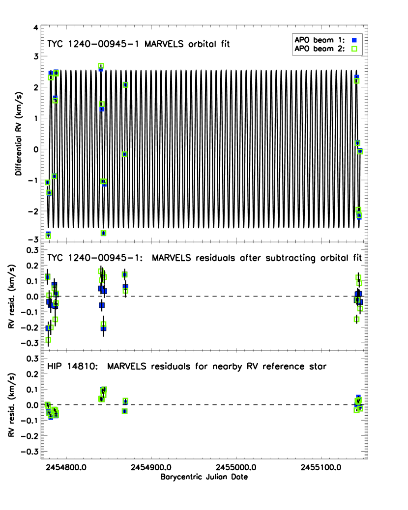
Figure 1: Top: MARVELS RV data and Keplerian orbital solution for TYC 1240-00945-1. Beam 1 is shown with blue filled squares, and beam 2 with green open squares. Center: The residuals for TYC 1240-00945-1, equal to the RVs from the top panel minus the orbital fit. Bottom: The residuals for HIP 14810, a star with a known two-planet RV signal, observed through a nearby fiber during the same exposures as those plotted for TYC 1240-00945-1.

In Table 1, we present the 20 radial velocities measured by the MARVELS instrument, and we show the RV curve as a function of time in Fig. 1. Both beams are shown, and even though the error bars plotted in Fig. 1 are photon-only and do not account for systematics (our procedure to determine more realistic error bars follows below), several of the beamwise pairs nonetheless agree within their error bars.

The MARVELS pipeline is still under development, and we find the RV scatter for other stars in the same field as TYC 1240-00945-1 (as well as for stars in other fields) is on average 2–3 times larger than the photon noise, on timescales greater than a month; presumably, most stars observed are not astrophysically variable at this level, indicating that the excess scatter is due to systematics (note we will discuss the expected RV jitter for TYC 1240-00945-1 in Section 6.4, since we need to determine the stellar properties first before searching for cases of similar stars in the literature). During pipeline development, we have examined the morphology of the RV residuals in the cases of several reference stars with known RV curves (either stable or planet-bearing) and found the systematic errors typically manifest in the form of month-to-month offsets at the level of tens of m s^-1, such that the RV data within any individual month fits the known RV curve much better than over multiple months. The offsets are often the same in direction and magnitude for both beams. These systematic errors may be due to imperfections in the detailed preprocessing of the images, because we do not see these systematics at the same level when analyzing simulated stellar data free of real-world image distortions. Since the exact factor by which the scatter exceeds the photon noise varies from star to star, we have decided to determine the excess scatter for the candidate at hand, to ensure that it falls in the typical range seen for other stars, and so is not responsible for the RV signal which we have interpreted as due to a companion.

Our procedure for estimating the magnitude of the systematic errors in the RV curve is as follows. We assume that the systematic errors can be well-modelled by applying a simple constant multiplicative scaling to the uncertainties derived from the photon noise alone. We choose to use a multiplicative scaling of the error bars instead of adding a systematic error in quadrature to the statistical error bars because during pipeline development, we found the increase in RV scatter above the photon noise level is larger for fainter stars than brighter stars, so adding systematic error in quadrature would not be able to capture the overall form of the extra error as a function of signal-to-noise ratio. We designate this multiplicative scaling factor the “quality factor” $Q$. We estimate $Q$ by performing a Keplerian fit to the RV dataset (with the raw pipeline photon-noise uncertainties), allowing for a linear trend with time. We then find the value of $Q$ such that the $\chi^{2}$/dof of the best-fit is equal to unity.

Following this error bar growth procedure, we found that the MARVELS RVs for TYC 1240-00945-1 were affected by systematics at levels of $Q_{\rm beam1}=2.21$ and $Q_{\rm beam2}=3.63$ for the two beams, respectively. Multiplying the statistical error bars by $Q$, we get a median scaled error bar of $92$ m s^-1 for beam 1 and $151$ m s^-1 for beam 2. After scaling the error bars, we performed a joint fit to beam 1 and beam 2 to provide a stronger constraint than a fit to either beam alone. The joint fit allows for different slopes and offsets between the two beams. This model is required because the two beams traveled through different parts of the instrument, and most importantly, experienced different optical path delays inside the interferometer (recall from Section 3.1 that there is a multiplicative factor that transforms fringe shift into radial velocity– this factor depends on the delay). The parameters of this final joint MARVELS orbital fit are given in Table 5 below, and the fit is overplotted with the data in Fig. 1. The uncertainties were determined using the Markov Chain Monte Carlo (MCMC) method (see, e.g., Ford 2006). Note the time is referenced to the time of inferior conjunction (i.e., the expected time of transit if the system is nearly edge-on), and is given as the Barycentric Julian Date (BJD) in the Barycentric Dynamical Time (TDB) standard (Eastman et al., 2010).

The $Q$ values for the two beams are consistent with that of a typical constant star’s $Q$, $\sim\!2-3$. We also checked the brighter planet-bearing reference star HIP 14810, which was observed on the same plate at the same time. Using the known RV model (Wright et al., 2009), we find this reference star has $Q_{\rm beam1}=5.29$ and $Q_{\rm beam2}=4.36$, with median statistical error bars of $9.1$ m s^-1 for beam 1 and $10.4$ m s^-1 for beam 2. The higher $Q$ for the brighter star is not an especially surprising result, since systematic noise sources that are independent of photon counts contribute a higher fraction of the total error when photon noise is small. Fig. 1 shows the residuals of HIP 14810 relative to the model curve, on the same scale as the RV residuals of TYC 1240-00945-1. These residuals demonstrate that we can recover the RV curve of a known planet-bearing star to a level at least as good as our TYC 1240-00945-1 fit. Hence, the level of systematic uncertainty we find for TYC 1240-00945-1 is not unusual for its field, and that level is small compared to the amplitude of RV variability we find for TYC 1240-00945-1 and attribute to a companion– MARVELS-1b.

4.2 HET AND SMARTS RADIAL VELOCITY DATA

To further confirm that RV variability is indeed due to a companion, as well as to confirm the basic parameters of the orbital fit, we compared the RV observations obtained from HET and SMARTS to those obtained by the MARVELS instrument. We found these RV data do verify the variability and periodicity, but the follow-up data sets comprise insufficient high quality data points to provide much additional refinement of the orbital fit parameters on top of the discovery data.

We first treated each RV dataset independently, computing a separate orbital fit and estimating $Q$ for the dataset using the procedure described above in §4.1. This gives the minimal error bars that would be consistent with any Keplerian orbital solution. We use these separate fits only for estimating the HET and SMARTS total error bars.

For the HET data we find $Q_{HET}=15.3$, which is high, but expected due to the preliminary nature of the pipeline used to reduce the data (see §3.4). We subtracted the RV model based on the MARVELS fit from the HET points and found that the residuals could be fit by a straight line (slope and offset) with $\chi^{2}=7.9$ and 7 degrees of freedom. Under the assumption that the errors are independent and normally distributed, this corresponds to a 33.4% probability of happening by chance, so there is no evidence to reject the hypothesis that the HET RVs are consistent with the MARVELS orbital fit.

For the SMARTS data we find $Q_{SMARTS}=1.50$. We subtracted the RV model based on the MARVELS fit from the SMARTS points and found that the residuals could be fit by a straight line (slope and offset) with $\chi^{2}=20.4$ and 6 degrees of freedom. Again assuming independent and normally distributed errors, this has a 0.23% probability of happening by chance, so there is strong evidence to reject the hypothesis that the SMARTS RVs are consistent with the MARVELS orbital fit. However, given that the HET and MARVELS RVs agree, we expect this discrepancy with the SMARTS data merely reflects evidence for unidentified systematics in the SMARTS data, which is not surprising, given the preliminary nature of the reduction of the SMARTS data (see §3.4).

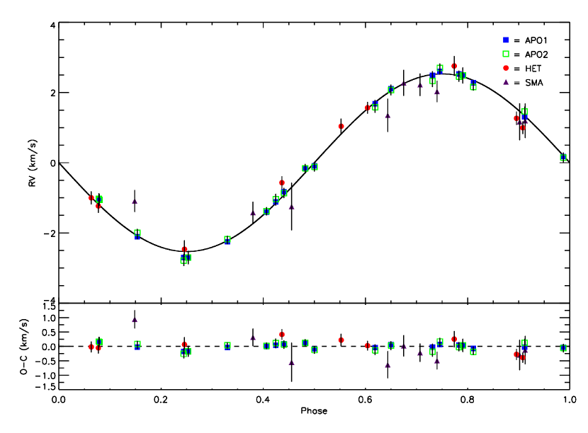
Figure 2: Phase-folded Keplerian orbital solution and RV residuals for TYC 1240-00945-1. Blue squares and green squares are MARVELS discovery data, red circles are HET data, and purple triangles are SMARTS data. Error bars have been scaled up by the methodology in §4.1. The bottom panel shows the residuals between the data points and the orbital solution. Note that the HET and SMARTS data were not used in the Keplerian fit, and so provide an independent check of the quality of the MARVELS data.

The four RV data sets are shown in Fig. 2, phase-folded to the fitted period and phase (as determined from the fit to the MARVELS data alone). This visually demonstrates the conclusion that the HET and SMARTS RV data confirm both the amplitude and phase of the variability. We then tried an orbital fit to all three telescopes’ data sets jointly, applying the same method that was used to jointly fit MARVELS beams 1 and 2, but now expanded to accommodate four RV data sets. We found that the new period and amplitude derived, using all the data sets combined, matched the values adopted in Table 5 to within the $1\sigma$ uncertainties, and furthermore, that the uncertainties themselves matched to within $\sim$10%.

5 MONITORING FOR PHOTOMETRIC VARIABILITY

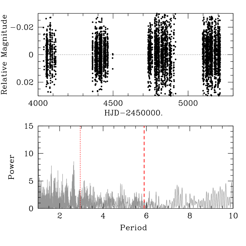
Figure 3: Top: KELT North light curve for TYC 1240-00945-1. Bottom: Lomb-Scargle periodogram of the KELT data, showing no evidence for any significant periodicities for periods of $P=1-10$ days, including the period of MARVELS-1b (vertical dashed line) and the first harmonic (vertical dotted line).

The KELT data for TYC 1240-00945-1 are displayed in Fig. 3, and show no evidence for variability. The final weighted RMS is 0.92%. A weighted Lomb-Scargle periodogram with floating mean (Lomb, 1976; Scargle, 1982) yields no significant peaks for periods of $1-10$ d, and in particular no evidence for any periodic variability near the period of the companion or the first harmonic. The improvement in $\chi^{2}$ for a sinusoidal fit at the period of the companion is only $\sim 0.1$ relative to a constant flux fit.

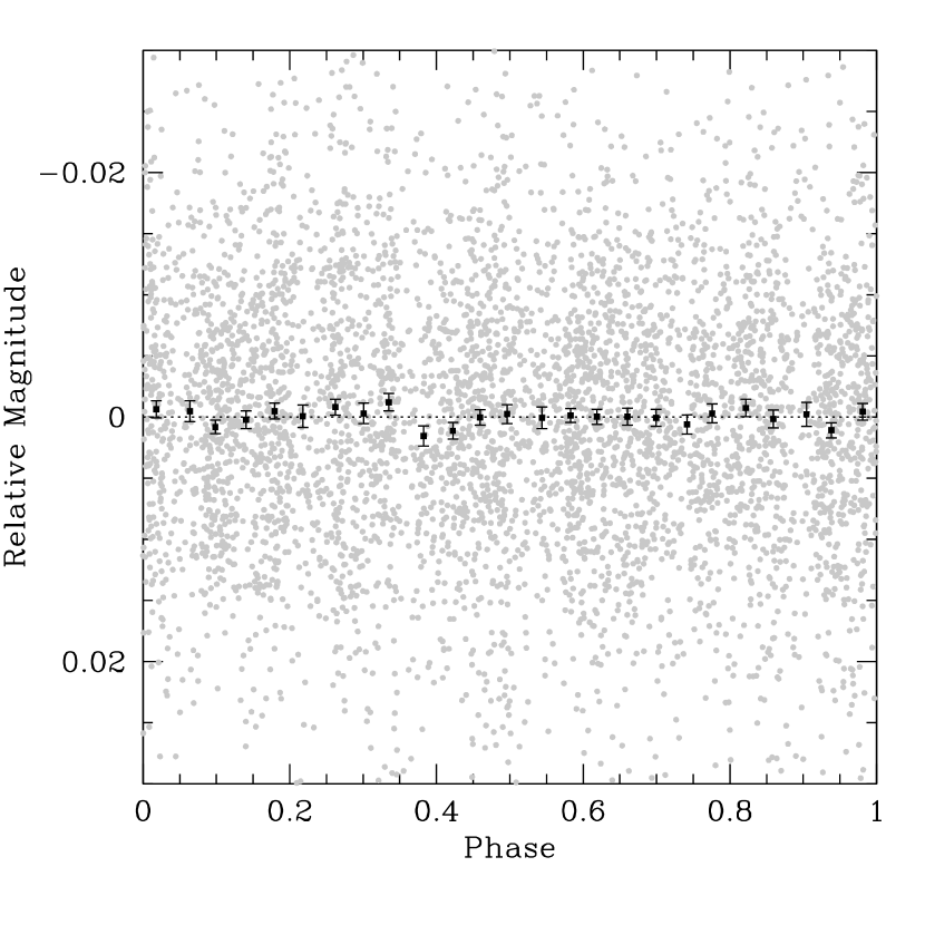
Figure 4: Grey points: the KELT light curve for TYC 1240-00945-1, phased to the period of MARVELS-1b ($5.8953$ days). Black points: the phased KELT light curve, binned using bin size $\Delta\phi=0.04$.

Fig. 4 shows the KELT light curve phased to the best-fit period of the companion ($5.8953$ d), as well as the phased light curve binned every 0.04 in phase (roughly the expected transit duration for a mid-latitude transit). The RMS of the binned curve is 0.059%, with a $\chi^{2}$/dof of 0.85. This is consistent with no correlated (red) noise at the level of the RMS, since with an average of $\sim\!200$ data points per phase bin, one would expect a factor of $\sim 15$ improvement for the binned RMS compared to the unbinned RMS. We can also place an upper limit of 0.050% on the maximum light curve variability at a period half that of the period from the RV orbital fit (at $\Delta\chi^{2}=9$), but this limit is insufficient to detect the expected amount of ellipsoidal variability for this candidate system. Using the equation in Table 2 of Pfahl et al. (2008), we calculate the ellipsoidal variation would only be 0.0019% in amplitude. Note the methods we use to calculate the physical parameters for the star and companion used in the equations in this section will be explained later, in §6.3.

We possess an ephemeris from the RV orbital fit to search for companion transits at the expected time. However, prior to our exposition of the Monte Carlo analysis using the RV information, let us first consider approximately what S/N to expect, calculated under the simplifying assumption of a random ephemeris (allowing us to write an analytic expression for the S/N). Based on the semimajor axis of $a=0.071$ AU for an edge-on system, the a priori transit probability for the companion is fairly high, $R_{*}/a=14.4$%. The expected duration of a central transit is $\sim\!R_{*}P/(\pi a)=6.49$ hours, and the expected depth is $\delta\!\sim\!(r/R_{*})^{2}=0.218\%(r/R_{Jup})^{2}$, where $r$ is the radius of the companion. Using these values, the expected S/N of a transit in the KELT data can be estimated,

$${S/N}\sim N^{1/2}\left(\frac{R_{*}}{\pi a}\right)^{1/2}\frac{\delta}{\sigma}\sim 3.5\left(\frac{r}{R_{Jup}}\right)^{2}$$ (1)

where $N=5036$ is the number of data points, and $\sigma\!\sim\!1\%$ is the typical uncertainty. Thus the detection of a transit using KELT data is challenging if the radius of the companion $r\!\lesssim\!R_{Jup}$, as is expected based on the likely age of the star (§7.1) and the minimum mass of the companion (Baraffe et al., 2003).

Detailed limits on transits are produced by using the same Monte Carlo analysis as described in Fleming et al. (2010) to incorporate our transit ephemeris from the RV data. Briefly, we use the distribution of companion periods and expected transit times from the MCMC chain derived from the fit to the MARVELS RV data (§4.1) to predict a distribution of transit times in the KELT data. For each link of the MCMC chain, we consider the uncertainty in the inferred radius of the primary due to the uncertainties in the spectroscopically measured $T_{\rm eff}$, $\log{g}$, and [Fe/H] (see §6.3), and we also consider a uniform range of transit impact parameters. For a given assumed radius for the companion, for each link we can then compute the expected transit curve using the routines of Mandel & Agol (2002), which are fit to the KELT dataset, computing the difference in $\chi^{2}$ relative to a constant flux fit to the data. This is repeated for each link in the Markov chain, as well as for a variety of different companion radii. We find that our best-fit transit light curve has $\Delta\chi^{2}\!\simeq\!-5$ relative to a constant flux fit. Based on analysis of the noise properties of the KELT light curve and the number of trials we performed searching for a transit, we estimate that $\Delta\chi^{2}\!\lesssim\!-16$ is generally indicative of a reliable detection, and thus this improvement is not significant.

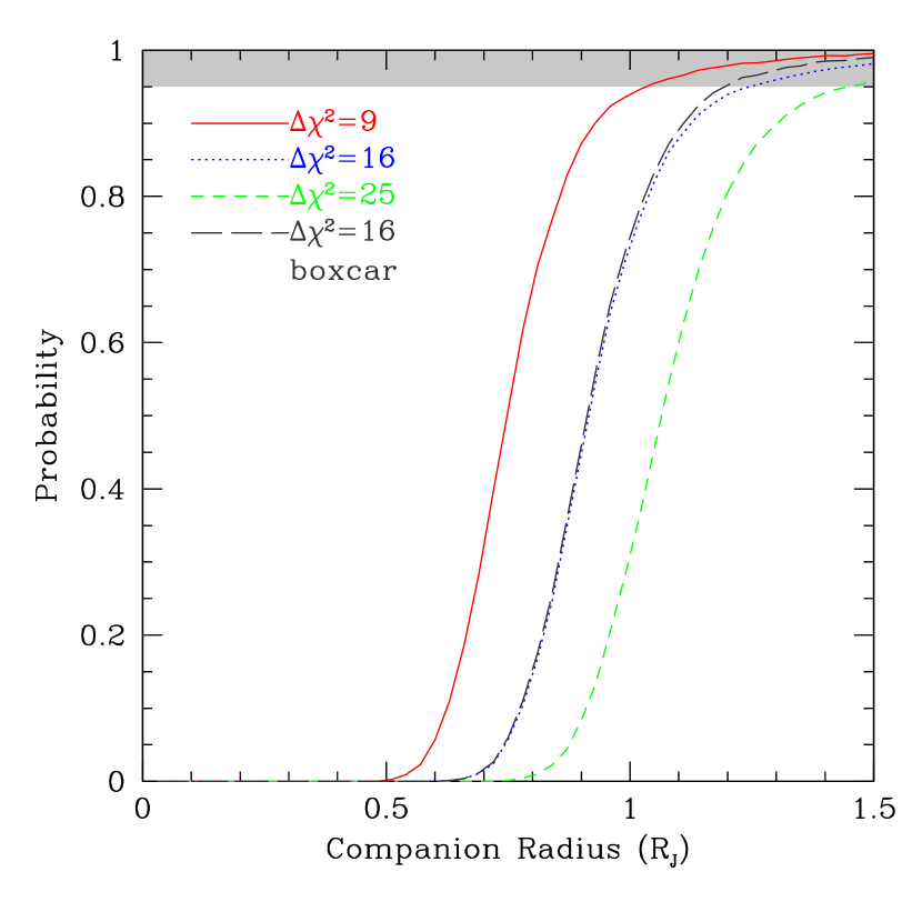
Figure 5: Probability that transits of MARVELS-1b are excluded at levels of $\Delta\chi^{2}=9$ (solid red), 16 (dotted blue), and 25 (dashed green), based on the analysis of the KELT photometric dataset, as a function of the radius of MARVELS-1b. Also shown is the case for $\Delta\chi^{2}=16$, but assuming a box-shaped transit (black, long dashes) instead of a limb-darkened light curve model.

We then determine the fraction of trials that lead to a $\Delta\chi^{2}$ greater than some threshold value. The results for $\Delta\chi^{2}$=9, 16, and 25 are shown in Fig. 5. We find that $\sim\!95$% of MCMC realizations of transit models for companion radii $>\!1.2\,R_{Jup}$ lead to fits to our light curve that are excluded by our data, in the sense of producing a $\Delta\chi^{2}$ that is worse by more than 16 relative to a constant fit. Therefore, we exclude with $\sim\!95$% confidence that the companion transits if it has a radius larger than $\sim\!1.2\,R_{Jup}$, and with $\sim\!75$% confidence if it has a radius larger $\sim\!R_{Jup}$. We conclude that while transits of a Jupiter-radius companion are unlikely, they are not definitively excluded.

6 STELLAR PARAMETERS

We have made multiple determinations of the stellar parameters of the host star, using several different sets of data and analysis methods, described below. The results are summarized in Table 6. We note that, although the different determinations are generally mutually consistent, the uncertainties associated with each are simply formal statistical uncertainties, which have not been externally calibrated. We expect that these formal uncertainties are likely underestimates of the true uncertainties. Therefore, we conservatively choose to report the median of the three highest resolution spectroscopic results as our best estimate of the stellar parameters, and take the uncertainty as the standard deviation of the three estimates. The final stellar parameters we adopt are effective temperature $T_{\rm eff}=6186\pm 92$ K, surface gravity $\log g=3.89\pm 0.07$ (cgs), and metallicity $\rm[Fe/H]=-0.15\pm 0.04$. These and other properties of the star are listed in Table 2.

6.1 Fitting of Spectral Lines

We analyzed the extracted APO 3.5-m spectra to determine the stellar properties in a careful hand-guided analysis according to the techniques used by Laws et al. (2003), which are described more fully (excepting recent improvements) in Gonzalez & Vanture (1998). Briefly, we make use of the line analysis code MOOG (Sneden 1973, updated version), the Kurucz (1993) LTE plane-parallel model atmospheres, and equivalent width (EW) measurements of 62 Fe I and 10 Fe II lines to determine the atmospheric parameters $T_{\rm eff}$, $\log g$, microturbulence $\xi_{t}$, and [Fe/H]. The formal uncertainties were calculated using the method in Gonzalez & Vanture (1998). The values are listed in Table 6.

As a check, we performed a second analysis of the APO spectra using the code Spectroscopy Made Easy (SME; see Valenti & Fischer, 2005). SME is an IDL-based program that uses synthetic spectra and least-squares minimization to determine the stellar parameters (e.g., $T_{\rm eff}$, $\log\,g$, [Fe/H], $v\,\sin\,i$, etc.) that best fit an observed spectrum. To constrain the stellar parameters, we analyzed three wavelength regions ($5160-5190$ Å, $6000-6200$ Å, and $6540-6590$ Å) used by Stempels et al. (2007). The first region is sensitive to $\log\,g$. The second region contains a large number of spectral features of different elements, and is sensitive to [M/H] and $v\,\sin\,i$. The third region contains H$\alpha$, and the broadening of the outer wings of this line is sensitive to $T_{\rm eff}$. We fitted all three regions simultaneously using SME to estimate the stellar parameters of TYC 1240-00945-1. SME was unable to determine $v\,\sin\,i$ to a level finer than the velocity resolution of the APO 3.5-m spectra ($\sim\!9$ km s^-1 at $R\!\sim\!31500$). We derived parameters that agreed with those determined from the same spectra using the Laws et al. (2003) methodology. The values are listed in Table 6.

The stellar parameters were also verified using the ESO 2.2-m FEROS spectra. Measurements of the equivalent widths were carried out automatically using the ARES code (Sousa et al., 2007). Given the high S/N and broad spectral range of the spectrum, results were obtained for a large number of atomic lines. However, after a careful inspection, only 21 Fe I and 9 Fe II lines (from the list in Table 2 of Ghezzi et al. (2010)) were considered sufficiently reliable to be used in the determination of the stellar parameters. Applying the technique described in Ghezzi et al. (2010), the following results were obtained: $T_{\rm eff}=6186\pm 82$ K, $\log g=4.01\pm 0.17$, $\xi_{t}=1.26\pm 0.17$ km s^-1, and [Fe/H]$=-0.14\pm 0.08$, where the formal uncertainties were calculated as in Gonzalez & Vanture (1998).

The projected rotational velocity of TYC 1240-00945-1 was estimated from the high-resolution FEROS spectrum using a technique similar to the one described in Ghezzi et al. (2009). The expectation from FEROS simulations is that the high oversampling of the line spread function for the FEROS spectrum allows us to probe to much lower $v\,\sin\,i$ than achievable with the APO 3.5-m spectra, even though the FEROS resolving power is only moderately higher. We measure $v\,\sin\,i$ by simultaneously fitting the macro-turbulence velocity and $v\,\sin\,i$ for three moderately strong Fe I spectral lines. A grid of synthetic spectra was generated, varying $v\,\sin\,i$, the macro-turbulence velocities and the adopted [Fe/H], the latter by 0.05 dex around the mean value given above. Small adjustments in the continuum level under 0.4% were allowed, to account for possible errors in the normalization process. In addition, small shifts in the central wavelengths of the Fe I lines were needed in order to properly match the observed lines. Values for $v\,\sin\,i$ and macro-turbulence were determined separately for each of the Fe I lines considered, based on standard reduced-$\chi^{2}$ minimization. The results obtained for the three Fe I lines were consistent, yielding a $v\,\sin\,i$ in the range $1.1-3.2$ km s^-1, and macro-turbulence in the range $4.5-4.7$ km s^-1. The latter values are in good agreement with the macroturbulence velocity derived from Equation 1 in Valenti & Fischer (2005) and $T_{\rm eff}=6186$ K. Our best estimate for $v\,\sin\,i$ was computed as the mean of the three values, yielding $v\,\sin\,i=2.2\pm 1.5$ km s^-1, where the uncertainty is the RMS value; this RMS scatter is approximately equal to the intrinsic uncertainty of the fitting procedure, which is typically $1-2$ km s^-1. Note that when we tried recovering $v\,\sin\,i$ from simulations of FEROS spectra at the S/N of the TYC 1240-00945-1 spectrum, we found that even lower $v\,\sin\,i$ would indeed be detectable at the FEROS resolution. However, as discussed below in §7.2, the lower 1$\sigma$ limit of 0.7 km s^-1 leads to a very long rotation period which is astrophysically unlikely; it is more probable that the true $v\,\sin\,i$ lies within the upper half of the estimated range from the fit.

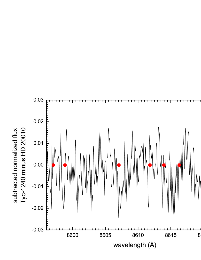
Figure 6: The normalized spectrum of TYC 1240-00945-1 minus the normalized spectrum of HD 20010 (an F8IV star with similar stellar parameters), in the wavelength range 8592-8626Å. Locations of some spectral lines of a late F subgiant are indicated by red dots.

We searched the FEROS spectra for any indication of spectral features from a secondary star blended with the primary, as might be expected if the RV signal were in fact caused by a nearly pole-on orbit of a low-mass stellar companion. To make a quantitative search for extra flux, we computed the difference of the normalized spectrum of TYC 1240-00945-1 with a template FEROS spectrum of the primary star of the binary HD 20010, a well-studied F subgiant (Balachandran, 1990; Santos et al., 2004; Luck & Heiter, 2005) with stellar parameters similar to those we derived for TYC 1240-00945-1. We examined the $8570-8630$ Å  region, where the spectrum has good continuum level determination, several spectral features (mostly due to Fe I), and where the contrast ratio between an M dwarf and the primary would be relatively high, before the red-end fall-off in detection efficiency of the FEROS spectra (in this range, the S/N per pixel of TYC 1240-00945-1 and HD 20010 were high: 180 and 390, respectively). From the Pickles (1998) low resolution spectral library, we computed the expected ratio of fluxes between F8IV and M0V stars over this wavelength range to be 1.5%. We would expect that ratio to manifest as a difference in line ratios between the template and target spectra, with the M dwarf’s flux filling up the cores of the F star’s lines. However, the difference spectrum shows no detectable systematic offsets at the locations of HD 20010’s lines; rather, the difference is evenly distributed around zero, with a standard deviation of 1.0%. The difference spectrum is shown in Fig. 6. This amount of deviation is expected since there is uncertainty in picking a template which would exactly match TYC 1240-00945-1. Thus there is no evidence for an M0V contaminating spectrum, although much cooler M dwarfs would provide less than 1.5% contaminating flux and might not be visible given the noise in our measurement.

6.2 Spectral Energy Distribution Fitting

As an additional check on the parameters of TYC 1240-00945-1, we performed a model atmosphere fit to the observed spectral energy distribution (SED) from the optical fluxes from HAO (§3.2) and near-IR fluxes from 2MASS (Skrutskie et al., 2006). The absolute photometric measurements in the $g^{\prime}r^{\prime}i^{\prime}JHK_{S}$ passbands (see Table 2) were converted to physical fluxes using the published SDSS and 2MASS zero-points, together with published color-dependent corrections to the passband effective wavelengths (Moro & Munari, 2000). The model atmospheres used in the fitting are the NextGen atmospheres of Hauschildt et al. (1999), which are gridded in $T_{\rm eff}$ by 100 K, in $\log g$ by 0.5 dex, and in [Fe/H] by 0.5 dex. We performed a least-squares fit of this model grid to the six flux measurements, with the extinction $A_{V}$ and the overall flux normalization as additional free parameters.

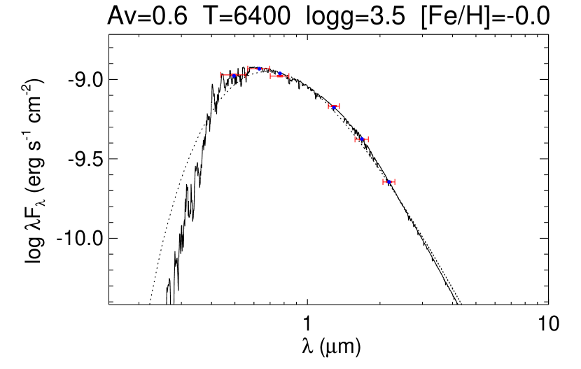
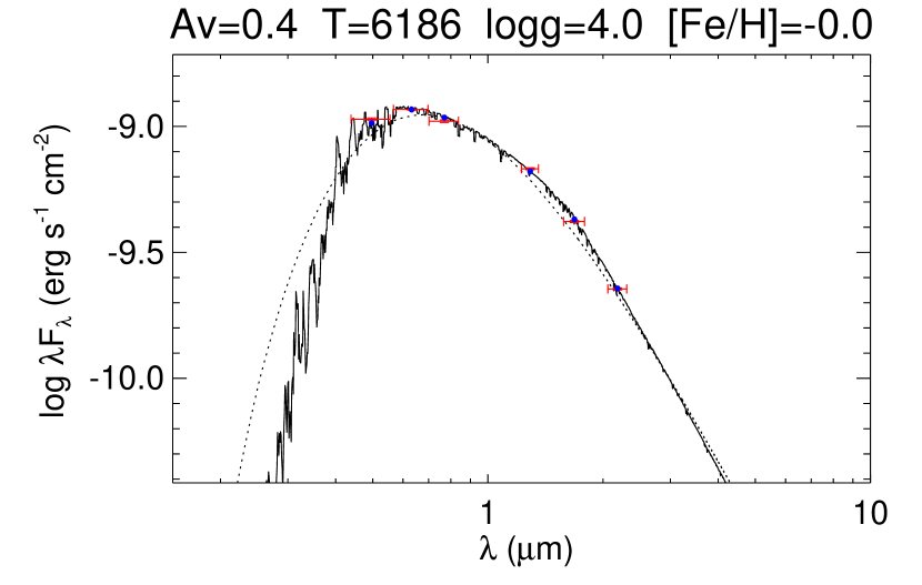
Figure 7: Top: NextGen model atmospheres SED fit to the color photometry of TYC 1240-00945-1, allowing all parameters to vary. Bottom: SED fit to the color photometry of TYC 1240-00945-1, with only $A_{V}$ and the normalization as variables ($T_{\rm eff}$, [Fe/H], and $\log g$ locked).

We initially allowed all of the variables– $T_{\rm eff}$, $\log g$, [Fe/H], $A_{V}$, and flux normalization– to be fit as free parameters. We limited the $A_{V}$ to a maximum of 0.65, corresponding to the maximum line-of-sight extinction as determined from the dust maps of Schlegel et al. (1998). The resulting fit is shown in Fig. 7, with $T_{\rm eff}=6400^{+400}_{-600}$ K, $A_{V}=0.6^{+0.05}_{-0.45}$, $\log g=3.5\pm 1.5$, and [Fe/H] $=0.0\pm 2.0$.

These values are consistent with those derived spectroscopically. However, the available photometry does not strongly constrain the stellar parameters as there is a very strong degeneracy in the SED fit between $T_{\rm eff}$ and $A_{V}$, due to the lack of absolute flux measurements at wavelengths bluer than $0.5$ $\mu$m. Thus, we re-fit the fluxes with $T_{\rm eff}$ fixed at the spectroscopic value of $6186$ K, [Fe/H] fixed at $0.0$, and $\log g$ fixed at $4.0$; the only remaining free parameters are $A_{V}$ and the normalization. In this way we use the photometry to strongly constrain the line-of-sight extinction. The resulting best fit, with $A_{V}=0.40\pm 0.05$, is displayed in Fig. 7.

Adopting this $A_{V}$, which implies $E(B-V)=0.13$ using the reddening law of Bessell & Brett (1988), we can check $T_{\rm eff}$ from the broadband colors alone, using the recent color calibrations of Casagrande et al. (2010). For example, from the $J-K_{S}$ color we find $T_{\rm eff}=6147$ K, while from the $V-K_{S}$ color we obtain $T_{\rm eff}=6299$ K. Thus, given a reasonable estimate of $A_{V}$, even when we use individual colors instead of fitting them all simultaneously, the $T_{\rm eff}$ estimates are consistent with the spectroscopically determined value to within $\sim\!100$ K.

6.3 Final Determination of the Stellar Parameters and Companion Parameters

We determine the mass and radius of the parent star, TYC 1240-00945-1, from $T_{\rm eff}$, $\log g$, and [Fe/H] using the empirical polynomial relations of Torres et al. (2010), which were derived from a sample of eclipsing binaries with precisely measured masses and radii. We estimate the uncertainties in $M_{*}$ and $R_{*}$ by propagating the uncertainties in $T_{\rm eff}$, $\log g$, and [Fe/H] (see Table 2) using the covariance matrices of the Torres et al. (2010) relations kindly provided by G. Torres. Also, since the polynomial relations of Torres et al. (2010) were derived empirically, the relations were subject to some intrinsic scatter, which we add in quadrature to the uncertainties propagated from the stellar parameter measurements. The final stellar mass and radius values we obtain in this way are $M_{*}=1.37\pm 0.11\,M_{\odot}$ and $R_{*}=2.20^{+0.25}_{-0.22}\,R_{\odot}$.

Using the derived value of $M_{*}$, we estimate a minimum mass (i.e., for $\sin\,i=1$ where $i$ is the orbital inclination) for the companion, MARVELS-1b, of $m_{\rm min}=28.0\pm 1.5\,M_{Jup}$, where the uncertainty is dominated by the uncertainty in the primary mass. In fact, the mass function,

$$\frac{(m\sin i)^{3}}{(M_{*}+m)^{2}}\,\propto\,K(1-e^{2})^{1/2}P^{1/3},$$ (2)

is more precisely determined. We find $(m\sin i)^{3}/(M_{*}+m)^{2}=(9.75\pm 0.32)\times 10^{-6}\,M_{\odot}$. With our adopted value of $M_{*}$, we can also estimate the semimajor axis $a=0.071\pm 0.002\,{\rm AU}$, assuming an edge-on orbit; for less inclined orbits, the semimajor axis is larger.

The small minimum mass of the companion positions it as a good short-period brown dwarf desert candidate. In order for it to be a low-mass star rather than a brown dwarf, the orbital inclination would have to be close to face-on. In order to explore further the probability that the companion has a mass greater than the hydrogen burning limit, we conducted a Bayesian analysis to estimate the posterior probability distribution for the companion mass, using the methodology described in Section 7 of Fleming et al. (2010): an MCMC chain is constructed starting from a distribution of stellar parameters and error bars as adopted for TYC 1240-00945-1 in Table 2, stellar masses are determined using Torres et al. (2010), and companion masses are determined using a random distribution of inclinations. This analysis assumes a uniform distribution in $\cos\,i$, includes uncertainties on the orbital and host star parameters, and adopts priors on the luminosity ratio and mass ratio for the companion.

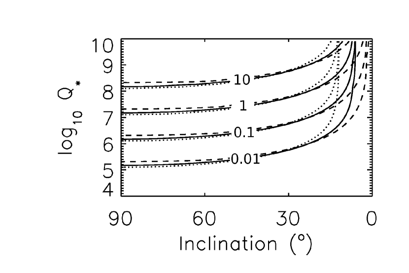
Figure 11: Contours of the time (in Gyr) to synchronize the primary’s rotational period to the orbital period, or for the companion to merge with its host star. Solid curves correspond to the best fit, dotted curves to the case with $v\,\sin\,i$, $M_{*}$, and $R_{*}$ each set at the tops of their $1\sigma$ uncertainty ranges, and dashed curves to the case with $v\,\sin\,i$, $M_{*}$, and $R_{*}$ each set at the bottoms of their $1\sigma$ uncertainty ranges. Merging is only possible in the latter case when $i\!\geq\!54^{\circ}$; therefore those portions of the dashed curves represent the time to merge.

Of course, the posterior distribution of the true companion mass depends on our adopted prior for the companion mass ratio distribution (e.g., Ho & Turner 2010). Given that few brown dwarf companions are known, the constraints on the companion mass ratio distribution in the mass regime of interest are poor. Indeed, this is what makes this object interesting, and this distribution is precisely what we would like to infer from a larger ensemble of similar detections. Nevertheless, we can adopt various simple and plausible forms for the mass ratio distribution, and then use these to infer posterior probability distributions for the true mass. From Doppler surveys for exoplanets, it is known that Jupiter-mass companions are significantly more common than brown dwarf companions, and that the frequency of planetary companions declines for larger masses, such that the mass function is roughly uniform in the logarithm of the planet mass for $m\lesssim 10~{}M_{J}$ (Cumming et al., 2008). It is not known if this form holds for companions with mass significantly larger than $\sim 10~{}M_{J}$, but it is clear that the frequency of companions in the brown dwarf regime must reach a minimum at some point and then rise again, given that M dwarf companions with masses just above the hydrogen burning limit are known to be more common than brown dwarf companions. Grether & Lineweaver (2006) found that this minimum (the driest part of the brown dwarf desert) occurs at a companion mass of $31_{-18}^{+25}~{}M_{J}$. Thus the minimum mass of MARVELS-1b is near the minimum of the companion mass function, and prior mass ratio distributions that are falling, flat, or perhaps rising shallowly in $\log{q}$ are all equally plausible (see Figure 11 of Grether & Lineweaver 2006).

We therefore consider five different priors on the companion mass ratio distribution: ${\rm d}N/{\rm d}\log{q}\propto q^{-1}$, $\propto\log{q}$, constant, $\propto q$, and $\propto q^{2}$. The first three are falling or constant with $\log{q}$, and the latter two are rising with $\log{q}$. From the results of Grether & Lineweaver (2006), we believe the first three are the most plausible, while the first four almost certainly bracket the likely range of distributions for companions close to the relevant regime. The resulting cumulative probabilities for the companion mass for the five different priors are plotted in Figure 8. For the three favored priors, we conclude that at $\gtrsim 90\%$ confidence the actual mass is below the hydrogen-burning limit. For the prior that is uniform in (linear) mass ratio, ${\rm d}N/{\rm d}\log{q}\propto q$, there is a $\sim 25\%$ probability that the companion is in fact a low-mass star, whereas it is only for the assumption of relatively steeply rising mass ratio distribution (${\rm d}N/{\rm d}\log{q}\propto q^{2}$) that the companion is more likely to be a star. Again, we do not believe such a distribution is very likely to be correct for this regime of companion mass, but given the poor constraints, we cannot absolutely exclude it either. Finally, we note that for the last two priors, the precise form of the posterior distribution depends on our imposed constraint on the luminosity ratio, which is somewhat uncertain.

With a reddening of $E(B-V)=0.13$ (§6.2), the system is evidently seen much of the way through the full reddening along this line of sight, which from the Schlegel et al. (1998) dust maps is $E(B-V)=0.186$. The physical distance of the system can be estimated from its luminosity and apparent magnitude. First we compute the bolometric magnitude of the star as $M_{\rm bol}=4.74-2.5\log(L/L_{\odot})$, where 4.74 is the bolometric magnitude of the Sun. The luminosity is calculated from the Stefan-Boltzmann law applied to the $T_{\rm eff}$ and stellar radius calculated above, and we adopt a $BC_{V}=-0.17$ as appropriate for its spectral type (e.g., Kenyon & Hartmann 1995). The absolute magnitude is therefore 2.91. Adopting $A_{V}=0.4\pm 0.05$ (§6.2), this yields a distance $d=280\pm 30$ pc.

6.4 Expected Stellar RV Jitter

Starspots and motions of the stellar surface are possible astrophysical sources of noise that can interfere with searches for companion RV signals. These sources are commonly referred to as “jitter”, and are explored by, e.g., Saar et al. (1998), Wright (2005), Lagrange et al. (2009), and Isaacson & Fischer (2010). For late F dwarfs of $B-V>0.5$, they find typical jitters in the $\sim$10 m s^-1 range, with the most extreme outliers at $\sim$100 m s^-1.

TYC 1240-00945-1 is slightly evolved, so one wonders whether it might experience larger jitter than for F dwarfs. However, it still lies at $B-V$ and $M_{V}$ below and redward of the instability strip (for a review of the position of the strip, see, e.g., Sandage & Tammann, 2006), and shows no signs of activity based on the time-series photometry (Section 5)– so one shouldn’t expect multi-periodic pulsations at the level of, e.g., the $\sim$400 m s^-1 RV jitter of the brown dwarf-hosting, instability strip, A9V star HD 180777 (Galland et al., 2006). Rather, F stars with stellar parameters similar to TYC 1240-00945-1 can be fairly quiet in terms of the RMS scatter attributable to RV jitter: $\sim$4-5 m s^-1 in the case of the F6 star HD 60532 (Desort et al., 2008), and $\sim$10 m s^-1 in the case of the F7 star HD 89744 (Korzennik et al., 2000).

We conclude that the levels of RV jitter expected for this combination of stellar parameters are too low to be responsible for the $K=2.533\pm 0.025$ km s^-1 of the TYC 1240-00945-1 RV signal, although they could be a contributor to the extra error we have regarded as systematics in the RV analysis.

7 DISCUSSION

7.1 Evolutionary state of the host star

In Fig. 9 we compare the spectroscopically measured $T_{\rm eff}$ and $\log g$ of TYC 1240-00945-1 (red error bars) against a theoretical stellar evolutionary track from the Yonsei-Yale (“Y²”) model grid (see Demarque et al. 2004 and references therein). The solid curve represents the evolution of a single star of mass $1.37\,M_{\odot}$ (the mass of TYC 1240-00945-1 inferred from the empirical calibration of Torres et al. 2010; see above) and metallicity of [Fe/H]=$-0.15$ (as determined spectroscopically), starting from the zero-age main sequence (lower left corner), across the Hertzsprung gap, and to the base of the red-giant branch. Symbols indicate various time points along the track, with ages in Gyr labeled. The dashed curves represent the same evolutionary track but for masses $\pm 0.11\,M_{\odot}$, representative of the $1\sigma$ uncertainty in the mass from the Torres et al. (2010) relation. The filled gray region between the mass tracks therefore represents the expected location of a star of TYC 1240-00945-1’s mass and metallicity as it evolves off the main sequence. We emphasize that we have not directly measured the mass of TYC 1240-00945-1, and thus we are not attempting to test the accuracy of the stellar evolutionary tracks. Rather, our goal is to use these tracks to constrain the evolutionary status of the TYC 1240-00945-1 system.

The spectroscopically measured $T_{\rm eff}$, $\log g$, and [Fe/H] place TYC 1240-00945-1 near the beginning of the subgiant phase, just prior to crossing the Hertzsprung gap to the base of the red giant branch, with an estimated age of $\sim\!3$ Gyr.

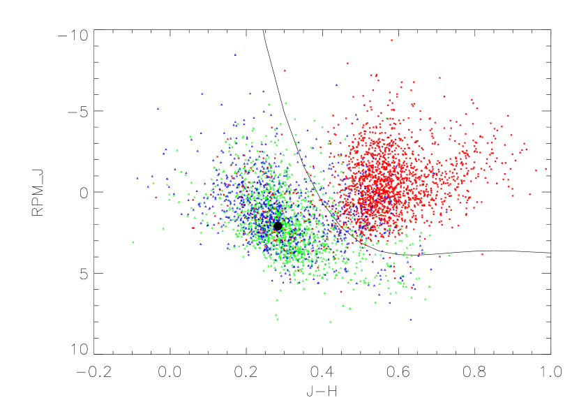
Figure 10: $J$-band reduced proper motion versus $J-H$ color. Stars from the RAVE DR2 (Zwitter et al., 2008) with galactic latitude, $20^{\circ}\!\leq\!|b|\!<\!30^{\circ}$, and with measured spectroscopic properties are shown. The RAVE stars are color coded by luminosity class such that giants ($\log g\!\leq\!3.5$) are red, dwarfs ($\log g\!>\!4.1$) are green, and subgiants ($4.1\!\geq\!\log g\!>\!3.5$) are blue. The polynomial relation (solid line) defined from Collier Cameron et al. (2007) discriminates the dwarf star population from the giant star population in this plane. TYC 1240-00945-1, plotted as the large black circle, is consistent with being a dwarf or subgiant.

We can also take advantage of the information provided by the MARVELS input catalog to place the host star on an RPM diagram, taking colors from the 2MASS catalog, and proper motions from the GSC2.3 (see Gould & Morgan 2003 for an example of how RPM can be used to help differentiate giants from dwarfs). In Fig. 10, we show that the $J$-band RPM ($RPM_{J}\equiv J+5\log\mu$) is most consistent with the host star being a dwarf or subgiant, as it falls well away from the region of the RPM diagram dominated by giant stars.

7.2 Tidal Effects

Given the relatively large mass ratio and short period of the TYC 1240-00945-1 system, tidal interactions between the star and MARVELS-1b could be important– given the roughly $\sim\!3$ Gyr age of the host star, is the system likely to be tidally synchronized? We follow exactly the same analysis of the tidal interaction as detailed in Fleming et al. (2010), which uses the tidal quality factor of the star, $Q^{\prime}_{*}$, as a free parameter in the equations for the decay of the companion’s semimajor axis over time and the relation of the primary’s rotational frequency to the companion’s orbital angular momentum (Eqs. 5 and 6 in Fleming et al. 2010); together, the equations permit a solution for the amount of time required for tidal synchronization. Note that if the primary’s rotation never synchronizes, the two bodies may merge (Counselman, 1973; Levrard et al., 2009; Jackson et al., 2009). As in Fleming et al. (2010), we have examined the tidal evolution of this system in the range $10^{4}\leq Q^{\prime}_{*}\leq 10^{10}$, for a range of values of the inclination of the secondary’s orbit to the line of sight from $i\!=\!0^{\circ}$ (face-on) to $i\!=\!90^{\circ}$ (edge-on), adjusting the mass and rotation period using the measured values of $v\,\sin\,i$ and $R_{*}$ from §6. We set the primary’s equator to be in the same plane as the secondary’s orbit, but this decision does not affect our results.

In Fig. 11 we show the synchronization and merging times from Eqs. 5 and 6 of Fleming et al. (2010), over the $Q^{\prime}_{*}$ and $i$ parameter space defined above. The curves are isochrones in the ($Q^{\prime}_{*}$, $i$) parameter space, so if the TYC 1240-00945-1 system has a ($Q^{\prime}_{*}$, $i$) combination that lies above a given isochrone $\tau_{sync/merge}$, then the system will take longer than $\tau_{sync/merge}$ to synchronize or merge. Isochrones are plotted for $\tau_{sync/merge}=0.01$, 0.1, 1, and 10 Gyr.

We consider three models: the best-fit stellar parameters (solid curves); one in which $v\,\sin\,i=3.7$ km s^-1, $M_{*}=1.43\,M_{\odot}$, and $R_{*}=2.44\,R_{\odot}$ (dotted curves); and one with $v\,\sin\,i=0.7$ km s^-1, $M_{*}=1.32\,M_{\odot}$, and $R_{*}=2.00\,R_{\odot}$ (dashed curves). The latter two cases represent models where the parameter sets were adjusted in opposite directions in an attempt to have the two models span a maximal amount of ($Q^{\prime}_{*},i$) parameter space, while still maintaining the parameters within the uncertainties. Thus, the uncertainty on the four synchronization/merging isochrones is approximately indicated by the region between the dotted and dashed lines (though it is not a perfect indication of the multi-parameter uncertainty envelope, as is evident from the fact that the dotted and dashed lines cross).

Note if one makes a trial assumption for the value of the inclination $i$, then given our measurement of $v\,\sin\,i$, one may infer the true rotational velocity $v$ of the stellar surface. At some small inclination, close to a face-on orbit, this will yield a $v$ so high that the primary’s rotational frequency is already spun up to tidal synchronization (and for the improbable case of an inclination even smaller than this, the primary’s rotational frequency is higher than the secondary’s orbital frequency, a scenario we do not explore here, but which would result in gradual spindown of the primary’s rotational frequency until it matched with the orbital frequency of the secondary). For each case of $v\,\sin\,i$ that we investigated, the value of the inclination which corresponds to present-day tidal synchronization is visible on Fig. 11 as a vertical asymptote towards which the isochrones converge. For inclinations closer to edge-on, the secondary still is in the process of spinning up the primary.

Next consider the best fit (solid curves) and maximum $v\,\sin\,i$ (dotted curves) cases. We find that for a wide range of low ($Q^{\prime}_{*}$, $i$) combinations, the secondary quickly spins the primary up to synchronization in less time than the $\sim\!3$ Gyr age of the host star. However, this alone, while suggestive, is not conclusive proof that such a synchronization has occurred. As this is an evolved F star, the radius has recently expanded, complicating any interpretations of the system’s history. Furthermore, for $Q^{\prime}_{*}\!\sim\!10^{7}$, the synchronization time is about the age of the system.

For the minimum $v\,\sin\,i$ cases (dashed curves), the rotational period of the star is very large, $\sim\!150$ days. While this period may not be physical, it is formally permitted by the observations. With such slow rotation, the companion may merge with the star before synchronization is finished. This possibility of the synchronization timescale exceeding the merging timescale occurs when $i\!\geq\!54^{\circ}$ (note there is no feature in Fig. 11 at the $i\!=\!54^{\circ}$ transition, because in our simplified model a companion can reach the stellar surface and synchronize the star’s rotation period, or move just inside the surface and merge). Undoubtedly the behavior of such a compact system is not well-modeled by Eqs. 5 and 6 of Fleming et al. (2010) , but we cannot rule out the possibility that MARVELS-1b will eventually merge with the host star.

8 SUMMARY

In a search through the first year of SDSS-III MARVELS data, we have discovered MARVELS-1b, a candidate brown dwarf companion to the $V\!\simeq\!10.6$ star TYC 1240-00945-1 with a velocity semiamplitude of $K=2.533\pm 0.025$ km s^-1 and an unusually short period of $5.8953\pm 0.0004$ d. Radial velocity data from several observatories confirm the Doppler variability, and high-resolution spectroscopic observations indicate that the host is a mildly evolved, slightly subsolar metallicity F star with $T_{\rm eff}=6186\pm 92$ K, $\log{g}=3.89\pm 0.07$, and [Fe/H]=$-0.15\pm 0.04$, with an inferred mass of $M_{*}=1.37\pm 0.11\,M_{\odot}$. The minimum mass of MARVELS-1b is $28.0\pm 1.5\,M_{Jup}$, implying that it is most likely in the brown dwarf regime. We see no evidence for spectral lines from the companion in the high-resolution spectra, implying that the companion is not an M dwarf with an orbit extremely close to pole-on. Comprehensive, precise relative photometry indicates no variability at a level of $\gtrsim\!1\%$ on time scales of hours to years. Phasing to the period of MARVELS-1b as well as the first harmonic, we can place an upper limit on the amplitude of coherent photometric variability of $\sim\!0.05\%$. Under many (but not all) of the potential combinations of system parameters, this short-period system is likely to have tidally synchronized, given the estimated $\sim\!3$ Gyr age of the host star.

The a priori transit probability of MARVELS-1b is quite high, $\sim\!14\%$. Although we find no evidence for transits, we also cannot definitively rule them out for likely MARVELS-1b radii of $r\!\sim\!R_{Jup}$. The transit ephemeris is $T_{C}=2454936.555\pm 0.024$ (BJD_TDB), with an expected transit depth of $\sim\!0.2\%(r/R_{Jup})^{2}$, and a duration of $\sim\!6.5$ hours for a central transit.

We believe this candidate highlights the great promise of MARVELS as a factory for finding the rare companions that populate the brown dwarf desert. The primary goal of the MARVELS survey is to monitor $\sim\!10^{4}$ main sequence and subgiant stars with velocity precision sufficient to detect Jovian companions with periods of less than a few years. As such, MARVELS is uniquely and exquisitely sensitive to massive but rare companions. MARVELS-1b is the first of a number of brown dwarf candidates we have identified in the MARVELS data obtained to date, and we expect to uncover several additional such systems as the survey progresses.

Table 1: SDSS-III MARVELS Radial Velocities for TYC 1240-00945-1

BJDTDB	Differential	Stat. err.	Scaled err.	Differential	Stat. err.	Scaled err.
	RVbeam1 (km s-1)	(km s-1)	(km s-1)	RVbeam2 (km s-1)	(km s-1)	(km s-1)
2454777.81083	-1.15	0.05	0.11	-1.16	0.05	0.18
2454778.78470	-2.81	0.04	0.10	-2.89	0.04	0.16
2454779.74062	-1.52	0.03	0.07	-1.49	0.03	0.12
2454781.65432	2.37	0.05	0.11	2.23	0.05	0.18
2454785.83590	-0.94	0.04	0.09	-0.96	0.04	0.15
2454786.88843	1.57	0.04	0.10	1.48	0.05	0.16
2454787.85523	2.42	0.04	0.09	2.35	0.04	0.15
2454787.90098	2.38	0.06	0.14	2.38	0.06	0.23
2454840.69407	2.49	0.04	0.08	2.60	0.04	0.13
2454841.67278	1.20	0.04	0.09	1.36	0.04	0.14
2454842.65535	-1.13	0.05	0.10	-1.13	0.05	0.17
2454843.68547	-2.83	0.05	0.12	-2.80	0.05	0.20
2454844.69581	-1.23	0.04	0.10	-1.14	0.04	0.16
2454868.61695	-0.26	0.04	0.08	-0.27	0.04	0.13
2454869.60690	1.99	0.04	0.10	1.97	0.04	0.16
2455141.74609	2.16	0.03	0.06	2.05	0.03	0.10
2455142.78463	0.06	0.04	0.09	0.04	0.04	0.15
2455143.76503	-2.22	0.03	0.07	-2.10	0.03	0.11
2455144.80421	-2.36	0.03	0.06	-2.28	0.03	0.10
2455145.80876	-0.20	0.04	0.08	-0.23	0.04	0.13

Table 2: TYC 1240-00945-1: Parameters of the Star

Parameter	Value
Spectral Type	F9IV-V
$g^{\prime}$	10.821 $\pm$ 0.013
$r^{\prime}$	10.436 $\pm$ 0.007
$i^{\prime}$	10.324 $\pm$ 0.013
$B$	11.230 $\pm$ 0.025
$V$	10.612 $\pm$ 0.025
$R_{c}$	10.242 $\pm$ 0.011
$I_{c}$	9.916 $\pm$ 0.011
$J_{2MASS}$	9.395 $\pm$ 0.018
$H_{2MASS}$	9.112 $\pm$ 0.016
$K_{2MASS}$	9.032 $\pm$ 0.017
$T_{\rm eff}$	6186 $\pm$ 92 K
$\log g$	3.89 $\pm$ 0.07 (cgs)
$\rm[Fe/H]$	-0.15 $\pm$ 0.04
Mass	1.37 $\pm$ 0.11 $M_{\odot}$
Radius	$2.20^{+0.25}_{-0.22}R_{\odot}$
$A_{V}$	$0.40\pm 0.05$
Distance	$280\pm 30$ pc
$v\,\sin\,i$	$2.2\pm 1.5$ km s-1

Table 3: HET Radial Velocities for TYC 1240-00945-1

BJDTDB	Differential RV	Stat. error	Scaled error
	(km s-1)	(km s-1)	(km s-1)
2455175.59389	0.78	0.02	0.29
2455177.61679	1.01	0.02	0.25
2455178.60575	-1.26	0.02	0.25
2455180.80563	-0.83	0.02	0.25
2455181.79358	1.31	0.01	0.23
2455182.79353	2.50	0.02	0.38
2455183.58448	0.74	0.02	0.24
2455184.58343	-1.49	0.02	0.26
2455185.57637	-2.72	0.02	0.34

Table 4: SMARTS Absolute Radial Velocities for TYC 1240-00945-1

BJDTDB	Absolute RV	Stat. error	Scaled error
	(km s-1)	(km s-1)	(km s-1)
2455052.89667	19.7	0.2	0.3
2455053.91287	18.9	0.3	0.4
2455084.78037	16.6	0.2	0.3
2455093.77977	19.9	0.2	0.3
2455109.72687	16.3	0.2	0.3
2455112.80387	18.8	0.3	0.5
2455139.64937	16.4	0.4	0.6
2455140.75867	19.0	0.3	0.4
2455164.71377	19.9	0.2	0.3

Table 5: MARVELS-1b: Parameters of the Companion

Parameter	Value
Minimum Mass	28.0 $\pm$ 1.5 $M_{Jup}$
$a$	0.071 $\pm$ 0.002 AU
$K$	2.533 $\pm$ 0.025 km s-1
$P$	5.8953 $\pm$ 0.0004 d
$T_{\rm{prediction\;for\;transit}}$	2454936.555 $\pm$ 0.024 (BJDTDB)
$e\cos\omega$	-0.015 ${}^{+0.010}_{-0.010}$
$e\sin\omega$	-0.003 ${}^{+0.008}_{-0.009}$

Table 6: TYC 1240-00945-1 Individual Determinations of Stellar Parameters

$T_{\rm eff}$	$\log g$	[Fe/H]	$\xi_{t}$	$v\sin i$	Notes
(K)	(cgs)		(km s-1)	(km s-1)
6186 $\pm$ 82	4.01 $\pm$ 0.17	-0.14 $\pm$ 0.08	1.26 $\pm$ 0.17	2.2 $\pm$ 1.5	High-res. (ESO 2.2-m)
6090 $\pm$ 74	3.89 $\pm$ 0.13	-0.21 $\pm$ 0.06	1.13 $\pm$ 0.18	-	High-res. (APO 3.5-m, hand redux)
6274 $\pm$ 112	3.89 $\pm$ 0.22	-0.15 $\pm$ 0.09	-	$\lesssim 9$	High-res. (APO 3.5-m, SME redux)
$6400^{+400}_{-600}$	3.5 $\pm$ 1.5	0.0 $\pm$ 2.0	-	-	SED fit to photometry

Figure 8: Cumulative probability that the mass of MARVELS-1b is less than a given mass, in units of solar masses. These probabilities account for the uncertainties and covariances between the parameters of the Keplerian orbital fit, the uncertainty in the host star mass, the assumption of a uniform distribution of $\cos\,i$, and the adoption of five different priors for the distribution of companion mass ratios ${\rm d}N/{\rm d}\log{q}$.

Figure 9: The evolutionary track for an object with $M=1.37\pm 0.11\,M_{\odot}$, at [Fe/H]=-0.15. Ages of 1.0, 2.0, 3.0, 3.2, 3.3, and 3.5 Gyr are indicated as dots. The possible tracks for up to a $1\sigma$ deviation in the mass are shown by the shaded region. The stellar parameters for TYC 1240-00945-1, with $1\sigma$ error bars, are shown by the cross.

References

- Alard & Lupton (1998) Alard, C., & Lupton, R. H. 1998, ApJ, 503, 325
- Armitage & Bonnell (2002) Armitage, P. J., & Bonnell, I. A. 2002, MNRAS, 330, L11
- Balachandran (1990) Balachandran, S. 1990, ApJ, 354, 310
- Baraffe et al. (2003) Baraffe, I., Chabrier, G., Barman, T. S., Allard, F., & Hauschildt, P. H. 2003, A&A, 402, 701
- Bessell & Brett (1988) Bessell, M. S., & Brett, J. M. 1988, PASP, 100, 1134
- Borucki et al. (1997) Borucki, W. J., Koch, D. G., Dunham, E. W., & Jenkins, J. M. 1997, in Astronomical Society of the Pacific Conference Series, Vol. 119, Planets Beyond the Solar System and the Next Generation of Space Missions, ed. D. Soderblom, 153
- Boss (2001) Boss, A. P. 2001, ApJ, 563, 367
- Butler et al. (1996) Butler, R. P., Marcy, G. W., Williams, E., McCarthy, C., Dosanjh, P., & Vogt, S. S. 1996, PASP, 108, 500
- Caballero et al. (2007) Caballero, J. A., Béjar, V. J. S., Rebolo, R., Eislöffel, J., Zapatero Osorio, M. R., Mundt, R., Barrado Y Navascués, D., Bihain, G., Bailer-Jones, C. A. L., Forveille, T., & Martín, E. L. 2007, A&A, 470, 903
- Campbell et al. (1988) Campbell, B., Walker, G. A. H., & Yang, S. 1988, ApJ, 331, 902
- Casagrande et al. (2010) Casagrande, L., Ramirez, I., Melendez, J., Bessell, M., & Asplund, M. 2010, ArXiv e-prints
- Chabrier (2002) Chabrier, G. 2002, ApJ, 567, 304
- Collier Cameron et al. (2007) Collier Cameron, A., Wilson, D. M., West, R. G., Hebb, L., Wang, X., Aigrain, S., Bouchy, F., Christian, D. J., Clarkson, W. I., Enoch, B., Esposito, M., Guenther, E., Haswell, C. A., Hébrard, G., Hellier, C., Horne, K., Irwin, J., Kane, S. R., Loeillet, B., Lister, T. A., Maxted, P., Mayor, M., Moutou, C., Parley, N., Pollacco, D., Pont, F., Queloz, D., Ryans, R., Skillen, I., Street, R. A., Udry, S., & Wheatley, P. J. 2007, MNRAS, 380, 1230
- Counselman (1973) Counselman, C. C., III. 1973, Icarus, 18, 1
- Cumming et al. (2008) Cumming, A., Butler, R. P., Marcy, G. W., Vogt, S. S., Wright, J. T., & Fischer, D. A. 2008, PASP, 120, 531
- del Peloso et al. (2005) del Peloso, E. F., da Silva, L., & Porto de Mello, G. F. 2005, A&A, 434, 275
- Demarque et al. (2004) Demarque, P., Woo, J., Kim, Y., & Yi, S. K. 2004, ApJS, 155, 667
- Desort et al. (2008) Desort, M., Lagrange, A., Galland, F., Beust, H., Udry, S., Mayor, M., & Lo Curto, G. 2008, A&A, 491, 883
- Dodson-Robinson et al. (2009) Dodson-Robinson, S. E., Veras, D., Ford, E. B., & Beichman, C. A. 2009, ApJ, 707, 79
- Eastman et al. (2010) Eastman, J. D., Siverd, R. J., & Gaudi, B. S. 2010, PASP, submitted (arXiv:1005.4415)
- Erskine & Ge (2000) Erskine, D. J., & Ge, J. 2000, in Astronomical Society of the Pacific Conference Series, Vol. 195, Imaging the Universe in Three Dimensions, ed. W. van Breugel & J. Bland-Hawthorn, 501
- Fleming et al. (2010) Fleming, S. W., Ge, J., Mahadevan, S., Lee, B., Eastman, J. D., Siverd, R. J., Gaudi, B. S., Niedzielski, A., Sivarani, T., Stassun, K. G., Wolszczan, A., Barnes, R., Gary, B., Cuong Nguyen, D., Morehead, R. C., Wan, X., Zhao, B., Liu, J., Guo, P., Kane, S. R., van Eyken, J. C., De Lee, N. M., Crepp, J. R., Shelden, A. C., Laws, C., Wisniewski, J. P., Schneider, D. P., Pepper, J., Snedden, S. A., Pan, K., Bizyaev, D., Brewington, H., Malanushenko, O., Malanushenko, V., Oravetz, D., Simmons, A., & Watters, S. 2010, ApJ, 718, 1186
- Ford (2006) Ford, E. B. 2006, ApJ, 642, 505
- Galland et al. (2006) Galland, F., Lagrange, A., Udry, S., Beuzit, J., Pepe, F., & Mayor, M. 2006, A&A, 452, 709
- Gary (2010) Gary, B. 2010, All-sky photometry: An iterative procedure, http://brucegary.net/AllSky/x.htm
- Ge (2002) Ge, J. 2002, ApJ, 571, L165
- Ge et al. (2002) Ge, J., Erskine, D. J., & Rushford, M. 2002, PASP, 114, 1016
- Ge et al. (2009) Ge, J., Lee, B., de Lee, N., Wan, X., Groot, J., Zhao, B., Varosi, F., Hanna, K., Mahadevan, S., Hearty, F., Chang, L., Liu, J., van Eyken, J., Wang, J., Pais, R., Chen, Z., Shelden, A., & Costello, E. 2009, in Society of Photo-Optical Instrumentation Engineers (SPIE) Conference Series, Vol. 7440, Society of Photo-Optical Instrumentation Engineers (SPIE) Conference Series
- Ge et al. (2008) Ge, J., Mahadevan, S., Lee, B., Wan, X., Zhao, B., van Eyken, J., Kane, S., Guo, P., Ford, E., Fleming, S., Crepp, J., Cohen, R., Groot, J., Galvez, M. C., Liu, J., Agol, E., Gaudi, S., Ford, H., Schneider, D., Seager, S., Weinberg, D., & Eisenstein, D. 2008, in Astronomical Society of the Pacific Conference Series, Vol. 398, Astronomical Society of the Pacific Conference Series, ed. D. Fischer, F. A. Rasio, S. E. Thorsett, & A. Wolszczan, 449
- Ge et al. (2006) Ge, J., van Eyken, J., Mahadevan, S., DeWitt, C., Kane, S. R., Cohen, R., Vanden Heuvel, A., Fleming, S. W., Guo, P., Henry, G. W., Schneider, D. P., Ramsey, L. W., Wittenmyer, R. A., Endl, M., Cochran, W. D., Ford, E. B., Martín, E. L., Israelian, G., Valenti, J., & Montes, D. 2006, ApJ, 648, 683
- Ghezzi et al. (2010) Ghezzi, L., Cunha, K., Smith, V. V., de Araújo, F. X., Schuler, S. C., & de la Reza, R. 2010, ApJ, 720, 1290
- Ghezzi et al. (2009) Ghezzi, L., Cunha, K., Smith, V. V., Margheim, S., Schuler, S., de Araújo, F. X., & de la Reza, R. 2009, ApJ, 698, 451
- Gizis et al. (2001) Gizis, J. E., Kirkpatrick, J. D., Burgasser, A., Reid, I. N., Monet, D. G., Liebert, J., & Wilson, J. C. 2001, ApJ, 551, L163
- Gonzalez & Vanture (1998) Gonzalez, G., & Vanture, A. D. 1998, A&A, 339, L29
- Gould & Morgan (2003) Gould, A., & Morgan, C. W. 2003, ApJ, 585, 1056
- Grether & Lineweaver (2006) Grether, D., & Lineweaver, C. H. 2006, ApJ, 640, 1051
- Gunn et al. (2006) Gunn, J. E., et al. 2006, AJ, 131, 2332
- Hauschildt et al. (1999) Hauschildt, P. H., Allard, F., & Baron, E. 1999, ApJ, 512, 377
- Ho & Turner (2010) Ho, S., & Turner, E. L. 2010, ApJ, submitted (arXiv:1007.0245)
- Høg et al. (2000) Høg, E., Fabricius, C., Makarov, V. V., Urban, S., Corbin, T., Wycoff, G., Bastian, U., Schwekendiek, P., & Wicenec, A. 2000, A&A, 355, L27
- Ida & Lin (2004) Ida, S., & Lin, D. N. C. 2004, ApJ, 616, 567
- Isaacson & Fischer (2010) Isaacson, H., & Fischer, D. A. 2010, ArXiv e-prints
- Jackson et al. (2009) Jackson, B., Barnes, R., & Greenberg, R. 2009, ApJ, 698, 1357
- Kaufer et al. (1999) Kaufer, A., Stahl, O., Tubbesing, S., Nørregaard, P., Avila, G., Francois, P., Pasquini, L., & Pizzella, A. 1999, The Messenger, 95, 8
- Kenyon & Hartmann (1995) Kenyon, S. J., & Hartmann, L. 1995, ApJS, 101, 117
- Korzennik et al. (2000) Korzennik, S. G., Brown, T. M., Fischer, D. A., Nisenson, P., & Noyes, R. W. 2000, ApJ, 533, L147
- Kovács et al. (2005) Kovács, G., Bakos, G., & Noyes, R. W. 2005, MNRAS, 356, 557
- Kratter et al. (2010) Kratter, K. M., Murray-Clay, R. A., & Youdin, A. N. 2010, ApJ, 710, 1375
- Kurucz (1993) Kurucz, R. L. 1993, VizieR Online Data Catalog, 6039, 0
- Kurucz et al. (1984) Kurucz, R. L., Furenlid, I., Brault, J., & Testerman, L. 1984, Solar flux atlas from 296 to 1300 nm
- Lagrange et al. (2009) Lagrange, A., Desort, M., Galland, F., Udry, S., & Mayor, M. 2009, A&A, 495, 335
- Landolt (1992) Landolt, A. U. 1992, AJ, 104, 340
- Laws et al. (2003) Laws, C., Gonzalez, G., Walker, K. M., Tyagi, S., Dodsworth, J., Snider, K., & Suntzeff, N. B. 2003, AJ, 125, 2664
- Lee et al. (2008) Lee, Y. S., Beers, T. C., Sivarani, T., Allende Prieto, C., Koesterke, L., Wilhelm, R., Re Fiorentin, P., Bailer-Jones, C. A. L., Norris, J. E., Rockosi, C. M., Yanny, B., Newberg, H. J., Covey, K. R., Zhang, H., & Luo, A. 2008, AJ, 136, 2022
- Levrard et al. (2009) Levrard, B., Winisdoerffer, C., & Chabrier, G. 2009, ApJ, 692, L9
- Lomb (1976) Lomb, N. R. 1976, Ap&SS, 39, 447
- Luck & Heiter (2005) Luck, R. E., & Heiter, U. 2005, AJ, 129, 1063
- Luhman & Muench (2008) Luhman, K. L., & Muench, A. A. 2008, ApJ, 684, 654
- Luhman et al. (2000) Luhman, K. L., Rieke, G. H., Young, E. T., Cotera, A. S., Chen, H., Rieke, M. J., Schneider, G., & Thompson, R. I. 2000, ApJ, 540, 1016
- Mandel & Agol (2002) Mandel, K., & Agol, E. 2002, ApJ, 580, L171
- Marcy & Butler (2000) Marcy, G. W., & Butler, R. P. 2000, PASP, 112, 137
- Matzner & Levin (2005) Matzner, C. D., & Levin, Y. 2005, ApJ, 628, 817
- Mayor et al. (2009) Mayor, M., Bonfils, X., Forveille, T., Delfosse, X., Udry, S., Bertaux, J., Beust, H., Bouchy, F., Lovis, C., Pepe, F., Perrier, C., Queloz, D., & Santos, N. C. 2009, A&A, 507, 487
- Mayor & Udry (2008) Mayor, M., & Udry, S. 2008, Physica Scripta Volume T, 130, 014010
- McCarthy & Zuckerman (2004) McCarthy, C., & Zuckerman, B. 2004, AJ, 127, 2871
- Metchev & Hillenbrand (2004) Metchev, S. A., & Hillenbrand, L. A. 2004, ApJ, 617, 1330
- Moro & Munari (2000) Moro, D., & Munari, U. 2000, A&AS, 147, 361
- Nidever et al. (2002) Nidever, D. L., Marcy, G. W., Butler, R. P., Fischer, D. A., & Vogt, S. S. 2002, ApJS, 141, 503
- Patel et al. (2007) Patel, S. G., Vogt, S. S., Marcy, G. W., Johnson, J. A., Fischer, D. A., Wright, J. T., & Butler, R. P. 2007, ApJ, 665, 744
- Pepper et al. (2007) Pepper, J., Pogge, R. W., DePoy, D. L., Marshall, J. L., Stanek, K. Z., Stutz, A. M., Poindexter, S., Siverd, R., O’Brien, T. P., Trueblood, M., & Trueblood, P. 2007, PASP, 119, 923
- Pfahl et al. (2008) Pfahl, E., Arras, P., & Paxton, B. 2008, ApJ, 679, 783
- Pickles (1998) Pickles, A. J. 1998, PASP, 110, 863
- Rafikov (2005) Rafikov, R. R. 2005, ApJ, 621, L69
- Ramsey et al. (1998) Ramsey, L. W., Adams, M. T., Barnes, T. G., Booth, J. A., Cornell, M. E., Fowler, J. R., Gaffney, N. I., Glaspey, J. W., Good, J. M., Hill, G. J., Kelton, P. W., Krabbendam, V. L., Long, L., MacQueen, P. J., Ray, F. B., Ricklefs, R. L., Sage, J., Sebring, T. A., Spiesman, W. J., & Steiner, M. 1998, in Presented at the Society of Photo-Optical Instrumentation Engineers (SPIE) Conference, Vol. 3352, Society of Photo-Optical Instrumentation Engineers (SPIE) Conference Series, ed. L. M. Stepp, 34
- Reid & Metchev (2008) Reid, I. N., & Metchev, S. A. 2008, The Brown Dwarf - Exoplanet Connection, ed. Mason, J. 115
- Saar et al. (1998) Saar, S. H., Butler, R. P., & Marcy, G. W. 1998, ApJ, 498, L153
- Sandage & Tammann (2006) Sandage, A., & Tammann, G. A. 2006, ARA&A, 44, 93
- Santos et al. (2004) Santos, N. C., Israelian, G., & Mayor, M. 2004, A&A, 415, 1153
- Scargle (1982) Scargle, J. D. 1982, ApJ, 263, 835
- Schlegel et al. (1998) Schlegel, D. J., Finkbeiner, D. P., & Davis, M. 1998, ApJ, 500, 525
- Scholz & Jayawardhana (2008) Scholz, A., & Jayawardhana, R. 2008, ApJ, 672, L49
- Shetrone et al. (2007) Shetrone, M., Cornell, M. E., Fowler, J. R., Gaffney, N., Laws, B., Mader, J., Mason, C., Odewahn, S., Roman, B., Rostopchin, S., Schneider, D. P., Umbarger, J., & Westfall, A. 2007, PASP, 119, 556
- Siverd et al. (2009) Siverd, R. J., Pepper, J., Stanek, K., Pogge, R. W., Gaudi, B. S., & DePoy, D. L. 2009, in IAU Symposium, Vol. 253, IAU Symposium, 350
- Skrutskie et al. (2006) Skrutskie, M. F., Cutri, R. M., Stiening, R., Weinberg, M. D., Schneider, S., Carpenter, J. M., Beichman, C., Capps, R., Chester, T., Elias, J., Huchra, J., Liebert, J., Lonsdale, C., Monet, D. G., Price, S., Seitzer, P., Jarrett, T., Kirkpatrick, J. D., Gizis, J. E., Howard, E., Evans, T., Fowler, J., Fullmer, L., Hurt, R., Light, R., Kopan, E. L., Marsh, K. A., McCallon, H. L., Tam, R., Van Dyk, S., & Wheelock, S. 2006, AJ, 131, 1163
- Smith et al. (2002) Smith, J. A., Tucker, D. L., Kent, S., Richmond, M. W., Fukugita, M., Ichikawa, T., Ichikawa, S., Jorgensen, A. M., Uomoto, A., Gunn, J. E., Hamabe, M., Watanabe, M., Tolea, A., Henden, A., Annis, J., Pier, J. R., McKay, T. A., Brinkmann, J., Chen, B., Holtzman, J., Shimasaku, K., & York, D. G. 2002, AJ, 123, 2121
- Sneden (1973) Sneden, C. A. 1973, Ph.D. thesis, THE UNIVERSITY OF TEXAS AT AUSTIN.
- Sousa et al. (2007) Sousa, S. G., Santos, N. C., Israelian, G., Mayor, M., & Monteiro, M. J. P. F. G. 2007, A&A, 469, 783
- Spagna et al. (2006) Spagna, A., Lattanzi, M. G., McLean, B., Bucciarelli, B., Carollo, D., Drimmel, R., Greene, G., Morbidelli, R., Pannunzio, R., Sarasso, M., Smart, R., & Volpicelli, A. 2006, Memorie della Societa Astronomica Italiana, 77, 1166
- Stassun et al. (2006) Stassun, K. G., Mathieu, R. D., & Valenti, J. A. 2006, Nature, 440, 311
- Stassun et al. (2007) Stassun, K. G., Mathieu, R. D., & Valenti, J. A. 2007, ApJ, 664, 1154
- Stempels et al. (2007) Stempels, H. C., Collier Cameron, A., Hebb, L., Smalley, B., & Frandsen, S. 2007, MNRAS, 379, 773
- Stetson (1987) Stetson, P. B. 1987, PASP, 99, 191
- Stoughton et al. (2002) Stoughton, C., et al. 2002, AJ, 123, 485
- Torres et al. (2010) Torres, G., Andersen, J., & Giménez, A. 2010, A&A Rev., 18, 67
- Tull (1998) Tull, R. G. 1998, in Society of Photo-Optical Instrumentation Engineers (SPIE) Conference Series, Vol. 3355, Society of Photo-Optical Instrumentation Engineers (SPIE) Conference Series, ed. S. D’Odorico, 387
- Uomoto et al. (1999) Uomoto, A., Smee, S., Rockosi, C., Burles, S., Pope, A., Friedman, S., Brinkmann, J., Gunn, J., Nichol, R., & SDSS Collaboration. 1999, in Bulletin of the American Astronomical Society, Vol. 31, Bulletin of the American Astronomical Society, 1501
- Valenti & Fischer (2005) Valenti, J. A., & Fischer, D. A. 2005, ApJS, 159, 141
- van Eyken et al. (2010) van Eyken, J. C., Ge, J., & Mahadevan, S. 2010, ApJS, 189, 156
- Vogt et al. (2002) Vogt, S. S., Butler, R. P., Marcy, G. W., Fischer, D. A., Pourbaix, D., Apps, K., & Laughlin, G. 2002, ApJ, 568, 352
- Wang et al. (2003) Wang, S., Hildebrand, R. H., Hobbs, L. M., Heimsath, S. J., Kelderhouse, G., Loewenstein, R. F., Lucero, S., Rockosi, C. M., Sandford, D., Sundwall, J. L., Thorburn, J. A., & York, D. G. 2003, in Society of Photo-Optical Instrumentation Engineers (SPIE) Conference Series, Vol. 4841, Society of Photo-Optical Instrumentation Engineers (SPIE) Conference Series, ed. M. Iye & A. F. M. Moorwood, 1145
- Wittenmyer et al. (2009) Wittenmyer, R. A., Endl, M., Cochran, W. D., Ramírez, I., Reffert, S., MacQueen, P. J., & Shetrone, M. 2009, AJ, 137, 3529
- Wright (2005) Wright, J. T. 2005, PASP, 117, 657
- Wright et al. (2009) Wright, J. T., Fischer, D. A., Ford, E. B., Veras, D., Wang, J., Henry, G. W., Marcy, G. W., Howard, A. W., & Johnson, J. A. 2009, ApJ, 699, L97
- York et al. (2000) York, D. G., et al. 2000, AJ, 120, 1579
- Zwitter et al. (2008) Zwitter, T., Siebert, A., Munari, U., Freeman, K. C., Siviero, A., Watson, F. G., Fulbright, J. P., Wyse, R. F. G., Campbell, R., Seabroke, G. M., Williams, M., Steinmetz, M., Bienaymé, O., Gilmore, G., Grebel, E. K., Helmi, A., Navarro, J. F., Anguiano, B., Boeche, C., Burton, D., Cass, P., Dawe, J., Fiegert, K., Hartley, M., Russell, K., Veltz, L., Bailin, J., Binney, J., Bland-Hawthorn, J., Brown, A., Dehnen, W., Evans, N. W., Re Fiorentin, P., Fiorucci, M., Gerhard, O., Gibson, B., Kelz, A., Kujken, K., Matijevič, G., Minchev, I., Parker, Q. A., Peñarrubia, J., Quillen, A., Read, M. A., Reid, W., Roeser, S., Ruchti, G., Scholz, R., Smith, M. C., Sordo, R., Tolstoi, E., Tomasella, L., Vidrih, S., & Wylie-de Boer, E. 2008, AJ, 136, 421