Gaussian Broadcast Channels with an Orthogonal and Bidirectional Cooperation Link

Abstract

This paper considers a system where one transmitter broadcasts a single common message to two receivers linked by a bidirectional cooperation channel, which is assumed to be orthogonal to the downlink channel. Assuming a simplified setup where, in particular, scalar relaying protocols are used and channel coding is not exploited, we want to provide elements of response to several questions of practical interest. Here are the main underlying issues: 1. The way of recombining the signals at the receivers; 2. The optimal number of cooperation rounds; 3. The way of cooperating (symmetrically or asymmetrically; which receiver should start cooperating in the latter case); 4. The influence of spectral resources. These issues are considered by studying the performance of the assumed system through analytical results when they are derivable and through simulation results. For the particular choices we made, the results sometimes do not coincide with those available for the discrete counterpart of the studied channel.

I Introduction

In the conventional broadcast channel (BC) introduced by [1], one transmitter sends independent messages to several receivers. The channel under investigation in this paper differs from the original BC for at least two reasons. First, the receivers can cooperate in order to enhance the overall system performance. Second, the users want to decode the same message. We will refer to this situation as the cooperative broadcast channel (CBC) with a single common message. For the sake of simplicity a 2-user CBC will be assumed. Note that the considered channel is also different from the original relay channel (RC) defined in [2], because each terminal not only acts as a relay but also as a receiver, which means that ultimately, the information message has to be decoded by both terminals. Additionally the cooperation channel between the two receivers is assumed to be bidirectional (versus unidirectional for the RC) and orthogonal to the downlink (DL) channels. Although their sub-optimality, orthogonal channels are often assumed for practical reasons (e.g. it is difficult/impossible to implement relay-receivers that receive and transmit at the same time in the same frequency band).

To the author’s knowledge the most significant contributions concerning the situation under investigation are [5][6][7][8][9][10]. The discrete broadcast channel with a bidirectional conference link and a single common message was originally studied by Draper et al. in [5]. The authors proposed a way of decoding the message in multiple rounds and applied their scheme to the binary erasure channel. The corresponding coding-decoding scheme is based on the use of auxiliary variables while a certain form of channel comparability is assumed through these variables. This channel has also been analyzed by [10] where the authors essentially proposed achievable rates based on the use of estimate-and-forward (EF) at both receivers and two-round cooperation schemes. The Gaussian counterpart of this channel has been studied in [8]. Showing the optimality of decode-and-forward for an unidirectional cooperation, the authors evaluated the exact loss due to the channel orthogonalization. For the bidirectional case, the proposed achievable rate is based on a combination of EF and decode-and-forward (DF) and shown to always outperform the pure EF-based solution (always for the 2-round decoding). Independently [7] exploited a similar approach to analyze the Gaussian relay channel with a bidirectional cooperation. The fading case has been partially treated in [6]. The diversity-multiplexing trade-off, achieved by using a “dynamic” version of decode-and-forward, is derived for the unidirectional cooperation case.

While the authors of [6][8][10] addressed situations where only one or two cooperation exchanges (or decoding rounds) are allowed, this paper focuses on the case where the number of exchanges is arbitrary. For the erasure channels, [5] and [9] have shown that the higher the number of exchanges the better the performance in terms of information rate. However the discrete channel analysis (including erasure channels) does not take into consideration the spectral resources aspect. As it will be seen, this point is in fact crucial and accounting for it can lead to markedly different conclusions from [5][9] concerning the optimum number of cooperation exchanges. Additionally, [5] and [9] only considered the information rate as a performance criterion whereas other criteria of interest can also be considered. Although assuming special cases of relaying protocols, this paper aims precisely at taking into account these two aspects for providing some insights to the following issues:

1. The way of recombining the signals at the receivers. Indeed, the receiver can combine the cooperation signal with either its downlink signal or the combiner output from the previous iteration. Also, the choice of the combining scheme (which depends on the assumed relaying protocol) will also be discussed.

2. The optimal number of the cooperation rounds. In contrast with the discrete case this number will be shown to be less than or equal to $2$ if the cooperation protocols are properly chosen.

3. The way of cooperating. The choice between symmetric and asymmetric can be made based on a simple discussion but it will also be illustrated by numerical results. Simulations will also indicate the relative importance of the order in which the receivers start to cooperate.

4. The influence of the spectral resources on the three mentioned issues will be assessed. Two different assumptions are made: ($\mathcal{H}_{1}$) The total system bandwidth is fixed; ($\mathcal{H}_{2}$) Only the downlink channel bandwidth is fixed.

In order to provide elements of response to these questions we will use a simplified approach. After presenting the used system model (sec. II), we will evaluate the exact equivalent signal-to-noise ratio (SNR) in the output of the maximum ratio combiner (MRC) for each user (sec. III) in the case where a scalar, memoryless and zero-delay amplify-and-forward protocol (AF) is assumed at both receivers. This will be done for several cooperation strategies. In order to assess the influence of the relaying protocol on the aforementioned issues we will also evaluate the system performance when DF is used at the relay. In this case, a more sophisticated combiner (namely a maximum likelihood detector – MLD), which is provided in Sec. IV, has to be used at the receivers. Based on the choice of different system performance criteria (sec. V-A), numerical and simulation analyses will be conducted (sec. V). Concluding remarks and possible extensions of the present work will be provided in Sec. VI.

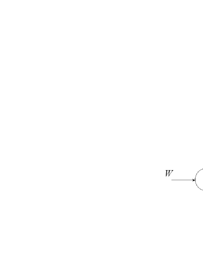
Figure 1: The cooperative broadcast channel with a single common message ($W$) and an orthogonal and bidirectional cooperation channel.

II System model

As mentioned in the previous section, the system under investigation (see Fig. 1) comprises one transmitter (source) and two receivers (destinations). The transmitted signal is denoted by $X$ and subject to a power constraint: $\mathbb{E}|X^{2}|\leq P$. Its bandwidth is denoted by $B_{DL}$. For the sake of simplicity, $X$ will be assumed to be a scalar quantity e.g. a Gaussian input or a quadrature amplitude modulation (QAM) symbol. Assuming an additive white Gaussian noise (AWGN) model for the different links of the system, the baseband downlink signals write:

$$\left\{\begin{array}[]{ccl}Y_{1}&=&X+Z_{1}\\ Y_{2}&=&X+Z_{2}\end{array}\right.$$ (1)

where for all $j\in\{1,2\}$, $Z_{j}\sim\mathbb{C}\mathcal{N}(0,n_{j}B_{DL})$, $n_{j}$ is the noise power spectral density for receiver $j$, and $I(Z_{1};Z_{2})=0$. We will assume that orthogonality between the downlink and cooperation channels is implemented by frequency division (FD). The bandwidth allocated to the cooperation channel between the two receivers is denoted by $B_{C}$. The cooperation channel can be divided into several sub-channels, each of them having a bandwidth equal to $\Delta B$. The two receivers cooperate by applying the same relaying strategy namely either the AF or DF protocol. Using the AF protocol imposes the condition $\Delta B=B_{DL}$ whereas $\Delta B$ and $B_{DL}$ can be chosen independently (or possibly through a compatibility constraint between the source and relay data rates) when DF is used for relaying . Regarding the spectral resources aspect, two different scenarios will be considered. In the first scenario we assume that $B_{DL}+B_{C}=const$ (Assumption $\mathcal{H}_{1}$). This corresponds to the situation where the total system bandwidth is fixed, which is generally assumed to fairly compare two systems before implementation. In the second scenario we assume that $B_{DL}=const$ (Assumption $\mathcal{H}_{2}$), which does not lead to fair comparisons in terms of bandwidth since the cooperation channel bandwidth can be chosen arbitrarily. The attention of the reader is drawn to the fact that, although unfair, this scenario still makes sense in the real life. For instance, consider the case where one wants to assess the benefits of cooperation by coupling two existing communication systems such as a DVB (digital video broadcasting) system and a cellular system. As modifying the DVB system downlink signal bandwidth would be a difficult/an impossible task, the second assumption, which amounts to extending the available bandwidth is more appropriate for comparing a DVB system with its terrestrial cooperation-based counterpart.

At last, we will assume scalar and zero-delay relaying. In real situations, this can be implemented for instance by re-synchronizing the downlink and cooperation signals at the receivers. The main advantage for assuming scalar protocols is that the additional complexity caused by the cooperation is low, it does not imply large decoding delays and some analytical results can be derived. As in [10], two main ways to cooperate are distinguished in this paper: the symmetric and asymmetric cooperation. The main distinction between these cooperation types is that for the symmetric cooperation the receivers exchange their cooperation signal simultaneously, while in the asymmetric cooperation the exchanges are done sequentially i.e. one receiver sends a cooperation signal at a given time. In the case where each receiver amplifies and forwards its received downlink signal the symmetric cooperation can be seen as a special case of the asymmetric cooperation.

III The case of amplify-and-forward

III-A Selected combining scheme

Let us consider the first cooperation round for the symmetric cooperation. Each receiver (e.g. receiver 1) amplifies and forwards his received downlink signal ($Y_{1}$ for receiver 1) to his partner (receiver 2). This is done simultaneously. Then each receiver (say receiver 2) has to combine its downlink signal with the cooperation signal received from his partner ($Y_{12}^{(1)}=a_{12}^{(1)}Y_{1}+Z_{12}^{(1)}$). To combine these signals we chose the MRC. The motivation for this choice is threefold. First, one of the features of the MRC is that it is simple. The MRC has also two properties. By definition it maximizes the equivalent SNR at its output. As shown in Appendix VII-A it also maintains the mutual information constant. The data processing theorem indicates that the MI between $X$ and the MRC output has to be less than or equal to the MI between $X$ and its (vector) input. It turns out that for the choice of weights maximizing the equivalent SNR, there is no loss of MI. At last, an additional motivation for the MRC is that it can be proved that using a more advanced combiner such as the MMSE will bring nothing more by taking into account the structure and statistics of the different signals. Now consider the second iteration of the cooperation procedure. Each receiver has at least two choices in terms of cooperation signals to be sent: it can continue to send its original downlink signal (Strategy $\mathcal{S}_{2}$) or it can send the MRC output from the previous iteration (Strategy $\mathcal{S}_{1}$). The first ($\mathcal{S}_{1}$) strategy is the counterpart of the strategy presented in [10] for the discrete CBC. Normally this strategy is intended to be better than the second one ($\mathcal{S}_{2}$) since the receiver can “de-noise” or remove some wrong information bits from the estimated data flow. Here, in our simplified setup (channel decoding is not exploited), the goal is to prove the intuition that sending to your partner what you received from him cannot improve the performance, which ultimately means that the second strategy is better than the first one.

III-B Received signals

Consider the case of the symmetric cooperation. To denote the signals of interest for a given cooperation round or iteration $i$, with $i\in\{1,...,K_{s}\}$, we will use the following notations:

$$\left\{\begin{array}[]{ccll}Y_{I}^{(i)}&=&\alpha_{I}^{(i)}X+Z_{I}^{(i)}\\ Y_{II}^{(i)}&=&\alpha_{II}^{(i)}X+Z_{II}^{(i)}\\ Y_{12}^{(i)}&=&a_{12}^{(i)}Y_{I}^{(j)}+Z_{12}^{(i)}\\ Y_{21}^{(i)}&=&a_{21}^{(i)}Y_{II}^{(j)}+Z_{21}^{(i)}\end{array}\right.$$ (2)

where $Y_{I}^{(i)}$ (resp. $Y_{II}^{(i)}$) corresponds to the MRC output at iteration $i$ and receiver 1 (resp. receiver 2), $a_{12}^{(i)}$, $a_{21}^{(i)}$ are the scalar AF protocol amplification gains, which are determined by the total cooperation powers available: $P_{12}$ at receiver 1 and $P_{21}$ at receiver 2. At last, $Y_{I}^{(0)}=Y_{1}$, $Y_{II}^{(0)}=Y_{2}$, $j=i-1$ for the strategy $\mathcal{S}_{1}$ and $j=0$ for the strategy $\mathcal{S}_{2}$. For the asymmetric cooperation, we will keep the same notations for the signals of interest as in the symmetric case. However, in contrast with the symmetric cooperation, combining operations take place at receiver 2 for odd indices $i$ only, and at receiver 1 for even indices $i$ only (under the assumption that receiver 1 starts relaying).

Whereas the notations are identical for the asymmetric and symmetric cooperation, the bandwidth of the cooperation channel is defined differently. If one denotes by $K_{s}$ the number of pairs of cooperation exchanges in the case of symmetric cooperation we have

$$\Delta B=\left|\begin{array}[]{ccccccc}\displaystyle{\frac{B}{2K_{s}+1}}&\mathrm{when}&B_{DL}+B_{C}&=&const.&\triangleq&B\\ B&\mathrm{when}&B_{DL}&=&const.&\triangleq&B,\end{array}\right.$$ (3)

and if one denotes by $K_{a}$ the number of cooperation exchanges in the case of asymmetric cooperation we have

$$\Delta B=\left|\begin{array}[]{ccccccc}\displaystyle{\frac{B}{K_{a}+1}}&\mathrm{when}&B_{DL}+B_{C}&=&const.&\triangleq&B\\ B&\mathrm{when}&B_{DL}&=&const.&\triangleq&B.\end{array}\right.$$ (4)

III-C Equivalent SNR analysis

The purpose of this section is to evaluate analytically the equivalent SNR at the MRC output after an arbitrary number of cooperation rounds for the two mentioned strategies. This allows us not only to compare them in terms of the SNR, but also to use this knowledge to evaluate other performance criteria presented in Sec. V-A.

III-C1 The case of the strategy $\mathcal{S}_{1}$

In this case, it turns out that it is not possible, in general, to express the equivalent SNR as a function of the sole channel parameters ($P,P_{12},n_{1},...$). In fact the equivalent SNR has to be determined recursively. The purpose of Theorem III.1 (see Appendix VII-B ) is precisely to provide this relationship, both for the asymmetric and the symmetric cooperation types. Before providing this theorem and the two underlying propositions, we need to mention and detail one important point regarding the interest in these results. First, let us consider the case where the system bandwidth is fixed. Imposing $\Delta B=\frac{B}{K+1}$ (with $K=K_{a}$ or $K=2K_{s}$ depending on the context) allows us to perform fair comparisons in terms of spectral resources whatever the value for $K$. However, the cases $K=0$, $K=1$ and $K=2$ do never correspond to fair comparisons in terms of power since they respectively correspond to $(P,P_{12}=0,P_{21}=0)$, $(P,P_{12},P_{21}=0)$ and $(P,P_{12},P_{21})$. For $K\geq 2$ the comparisons are spectrally fair because the total cooperation powers are kept fixed.

Theorem III.1

(General expression for the equivalent SNRs). Assume that $n_{1}<n_{2}$ and receiver 2 performs the MRC task in the first place if asymmetric cooperation is considered. For iteration $i\in\{1,...,K\}$ the corresponding weights are denoted by $w_{2}^{(i)}$ (weighting the MRC output at iteration $i-1$) and $w_{12}^{(i)}$ (weighting the cooperation signal). For receiver 1 the weights are denoted by $w_{1}^{(i)}$, $w_{21}^{(i)}$. Denote by $Y_{I}^{(i)}=\alpha_{I}^{(i)}X+Z_{I}^{(i)}$ (resp. $Y_{II}^{(i)}=\alpha_{II}^{(i)}X+Z_{II}^{(i)}$) the signal at MRC output for receiver 1 (resp. receiver 2) and iteration $i$, with $Z_{I}^{(i)}\sim\mathcal{N}(0,N_{I}^{(i)})$ (resp. $Z_{II}^{(i)}\sim\mathcal{N}(0,N_{II}^{(i)})$). Let $\rho_{I}^{(i)}$ (resp. $\rho_{II}^{(i)}$) be the signal-to-noise ratio associated with the signal $Y_{I}^{(i)}$ (resp. $Y_{II}^{(i)}$). The SNRs $\rho_{I}^{(i)}\triangleq\displaystyle{\frac{\mathcal{S}_{I}^{(i)}}{\mathcal{T}_{I}^{(i)}}}$ and $\rho_{II}^{(i)}\triangleq\displaystyle{\frac{\mathcal{S}_{II}^{(i)}}{\mathcal{T}_{II}^{(i)}}}$ can be determined recursively as follows:

$$\begin{array}[]{ccl}\mathcal{S}_{II}^{(i)}&=&\displaystyle{\alpha_{I}^{(i-1)}\alpha_{II}^{(i-1)}\left(e^{(i-1)}+e^{(i-1),*}\right)\rho_{I}^{(i-1)}\rho_{II}^{(i-1)}\rho_{12}}\displaystyle{-\left(\alpha_{I}^{(i-1)}\alpha_{II}^{(i-1)}\right)^{2}P\left[\rho_{II}^{(i-1)}\left(1+\rho_{I}^{(i-1)}\right)\right.}\\ &&\displaystyle{+\left.\rho_{12}\left(\rho_{I}^{(i-1)}+\rho_{II}^{(i-1)}\right)\right]}\\ \mathcal{T}_{II}^{(i)}&=&\displaystyle{\frac{e^{(i-1)}e^{(i-1),*}}{P}\rho_{I}^{(i-1)}\rho_{II}^{(i-1)}\rho_{12}}\displaystyle{-\left(\alpha_{I}^{(i-1)}\alpha_{II}^{(i-1)}\right)^{2}P\left(1+\rho_{12}\right)}-\displaystyle{\left(\alpha_{I}^{(i-1)}\right)^{2}N_{II}^{(i-1)}\rho_{I}^{(i-1)}\rho_{II}^{(i-1)}}\end{array}$$ (5)

where $\rho_{12}=\displaystyle{\frac{P_{12}}{n_{12}\Delta B}}$, $k$ is a constant depending on the cooperation scheme (asymmetric or symmetric), $(.)^{*}$ denotes the conjugate, $e^{(0)}=0$, $N_{I}^{(0)}=N_{1}$, $N_{II}^{(0)}=N_{2}$, $\rho_{I}^{(0)}=P/N_{1}$, $\rho_{II}^{(0)}=P/N_{2}$, $\alpha_{I}^{(0)}=\alpha_{II}^{(0)}=1$. The amplification gains are defined by: $a_{12}^{(i)}=\sqrt{\frac{P_{12}^{(i)}}{(\alpha_{I}^{(i-1)})^{2}P+N_{I}^{(i-1)}}}$, $a_{21}^{(i)}=\sqrt{\frac{P_{21}^{(i)}}{(\alpha_{II}^{(i-1)})^{2}P+N_{II}^{(i-1)}}}$ and $P_{12}^{(i)}$, $P_{21}^{(i)}$ are the available cooperation powers per subchannel. For the SNR $\rho_{I}^{(i)}$ do the following changes for the indices: $I\leftrightarrow II$ and $1\leftrightarrow 2$.

The expressions of the signals coefficients $\alpha_{I}^{(i)}$, $\alpha_{II}^{(i)}$, the cooperation powers per subchannel $P_{12}^{(i)}$ , $P_{21}^{(i)}$ and the equivalent noise powers $N_{I}^{(i)}$, $N_{II}^{(i)}$ depend on the cooperation type. Expressing these quantities is the purpose of the following two propositions.

Proposition III.2

(MRC weights for the symmetric cooperation). For the symmetric cooperation the MRC weights can be shown to be:

$$\left\{\begin{array}[]{ccl}w_{12}^{(i)}&=&a_{12}^{(i)}\alpha_{I}^{(i-1)}N_{II}^{(i-1)}-a_{12}^{(i)}\alpha_{II}^{(i-1)}e^{(i-1)}\\ w_{2}^{(i)}&=&\left[(a_{12}^{(i)})^{2}N_{I}^{(i-1)}+N_{12}^{(i)}\right]\alpha_{II}^{(i-1)}-(a_{12}^{(i)})^{2}\alpha_{I}^{(i-1)}e^{(i-1),*}\\ w_{21}^{(i)}&=&a_{21}^{(i)}\alpha_{II}^{(i-1)}N_{I}^{(i-1)}-a_{21}^{(i)}\alpha_{I}^{(i-1)}e^{(i-1),*}\\ w_{1}^{(i)}&=&\left[(a_{21}^{(i)})^{2}N_{II}^{(i-1)}+N_{21}^{(i)}\right]\alpha_{I}^{(i-1)}-(a_{21}^{(i)})^{2}\alpha_{II}^{(i-1)}e^{(i-1)}\end{array}\right.$$ (6)

where

• $e^{(i-1)}\triangleq E\left[Z_{I}^{(i-1)}Z_{II}^{(i-1),*}\right]$ with

  $$\begin{array}[]{ccl}e^{(i)}&=&w_{12}^{(i)}a_{12}^{(i)}w_{1}^{(i)}N_{I}^{(i-1)}+w_{21}^{(i)}a_{21}^{(i)}w_{2}^{(i)}N_{II}^{(i-1)}\\ &&+\left[w_{1}^{(i)}w_{2}^{(i)}+w_{12}^{(i)}a_{12}^{(i)}w_{21}^{(i)}a_{21}^{(i)}\right]e^{(i-1)},\end{array}$$ (7)

• for all $i\in\{1,...,K_{s}\}$ the useful signal coefficients are given by

  $$\left\{\begin{array}[]{ccl}\alpha_{I}^{(i)}&=&w_{21}^{(i)}a_{21}^{(i)}\alpha_{II}^{(i-1)}+w_{1}^{(i)}\alpha_{I}^{(i-1)}\\ \alpha_{II}^{(i)}&=&w_{12}^{(i)}a_{12}^{(i)}\alpha_{I}^{(i-1)}+w_{2}^{(i)}\alpha_{II}^{(i-1)},\end{array}\right.$$ (8)

• the cooperation powers per subchannel are for all $i\in\{1,...,K_{s}\}$ given by

  $$\left\{\begin{array}[]{ccc}P_{12}^{(i)}&=&\displaystyle{\frac{P_{12}}{K_{s}}}\\ P_{21}^{(i)}&=&\displaystyle{\frac{P_{21}}{K_{s}}},\end{array}\right.$$ (9)

• the equivalent noise powers $N_{I}^{(i)}$, $N_{II}^{(i)}$ are determined through

  $$\left\{\begin{array}[]{ccc}Z_{I}^{(i)}&=&w_{21}^{(i)}a_{21}^{(i)}Z_{II}^{(i-1)}+w_{21}^{(i)}Z_{21}^{(i)}+w_{1}^{(i)}Z_{I}^{(i-1)}\\ Z_{II}^{(i)}&=&w_{12}^{(i)}a_{12}^{(i)}Z_{I}^{(i-1)}+w_{12}^{(i)}Z_{12}^{(i)}+w_{2}^{(i)}Z_{II}^{(i-1)}.\end{array}\right.$$ (10)

• for all $i\in\{1,...,K_{s}\}$: $N_{12}^{(i)}=n_{12}\Delta B$ and $N_{21}^{(i)}=n_{21}\Delta B$

• the constant $k$ of Theorem III.1 equals $\displaystyle{\frac{2K_{s}+1}{K_{s}}}$.

Proposition III.3

(MRC weights for the asymmetric cooperation). For the asymmetric cooperation the MRC weights can be shown to coincide with that of Proposition III.2 where

• $e^{(i-1)}\triangleq E\left[Z_{I}^{(i-1)}Z_{II}^{(i-1),*}\right]$ with

  $$e^{(i)}=\left|\begin{array}[]{cc}w_{1}^{(i)}e^{(i-1)}+w_{21}^{(i)}a_{(21)}^{(i)}N_{II}^{(i-1)}&\ for\ i\ even\\ w_{2}^{(i)}e^{(i-1)}+w_{12}^{(i)}a_{(12)}^{(i)}N_{I}^{(i-1)}&\ for\ i\ odd,\end{array}\right.$$ (11)

• the useful signal coefficients are given by

  $$\alpha_{I}^{(i)}=\left|\begin{array}[]{cc}w_{21}^{(i)}a_{21}^{(i)}\alpha_{II}^{(i-1)}+w_{1}^{(i)}\alpha_{I}^{(i-1)}&\ for\ i\ even\\ \alpha_{I}^{(i-1)}&\ for\ i\ odd,\end{array}\right.$$ (12)

  $$\alpha_{II}^{(i)}=\left|\begin{array}[]{cc}\alpha_{II}^{(i-1)}&\ for\ i\ even\\ w_{12}^{(i)}a_{12}^{(i)}\alpha_{I}^{(i-1)}+w_{2}^{(i)}\alpha_{II}^{(i-1)}&\ for\ i\ odd,\end{array}\right.$$ (13)

• the cooperation powers per subchannel are for all $i\in\{1,...,K_{a}\}$

  $$P_{12}^{(i)}=\left|\begin{array}[]{cc}\displaystyle{\frac{2P_{12}}{K_{a}}}&for\ K_{a}\ even\\ \displaystyle{\frac{2P_{12}}{K_{a}+1}}&\ for\ K_{a}\ odd,\end{array}\right.$$ (14)

  $$P_{21}^{(i)}=\left|\begin{array}[]{cc}\displaystyle{\frac{2P_{21}}{K_{a}}}&\ for\ K_{a}\ even\\ \displaystyle{\frac{2P_{21}}{K_{a}-1}}&\ for\ K_{a}\ odd,\ K_{a}\geq 3,\end{array}\right.$$ (15)

• the equivalent noise powers $N_{I}^{(i)}$, $N_{II}^{(i)}$ are determined through

  $$Z_{I}^{(i)}=\left|\begin{array}[]{cc}w_{21}^{(i)}a_{21}^{(i)}Z_{II}^{(i-1)}+w_{21}^{(i)}Z_{21}^{(i)}+w_{1}^{(i)}Z_{I}^{(i-1)}&\ i\ even\\ Z_{I}^{(i-1)}&\ i\ odd,\end{array}\right.$$ (16)

  $$Z_{II}^{(i)}=\left|\begin{array}[]{cc}Z_{II}^{(i-1)}&\ i\ even\\ w_{12}^{(i)}a_{12}^{(i)}Z_{I}^{(i-1)}+w_{12}^{(i)}Z_{12}^{(i)}+w_{2}^{(i)}Z_{II}^{(i-1)}&\ i\ odd,\end{array}\right.$$ (17)

• for all $i\in\{1,...,K_{a}\}$: $N_{12}^{(i)}=n_{12}\Delta B$ and $N_{21}^{(i)}=n_{21}\Delta B$,

the constant $k$ of Theorem III.1 equals 1.

The theorem and propositions provided here are proved in Appendix VII-B,VII-C,VII-D.

III-C2 The case of the strategy $\mathcal{S}_{2}$

As the strategy $\mathcal{S}_{2}$ consists in always sending to the other receiver the downlink signal, it can be easily checked that the performance of the symmetric case with a number of pairs of cooperation rounds equal to $K_{s}$ is the same as the asymmetric case with $2K_{s}$ cooperation rounds. As the symmetric case is easier to expose and the derivations in both cases are similar, we restrict our attention to the symmetric case here. The received signal are particularly simple to express in the case of strategy $\mathcal{S}_{2}$:

$$\left\{\begin{array}[]{ccll}Y_{I}^{(i)}&=&\displaystyle{\left(w_{1}+\sum_{i=1}^{K_{s}}w_{21}^{(i)}a_{21}^{(K_{S})}\right)X+Z_{1}+\sum_{i=1}^{K_{s}}w_{21}^{(i)}Z_{2}+Z_{21}^{(i)}}\\ Y_{II}^{(i)}&=&\displaystyle{\left(w_{2}+\sum_{i=1}^{K_{s}}w_{12}^{(i)}a_{12}^{(K_{s})}\right)X+Z_{2}+\sum_{i=1}^{K_{s}}w_{12}^{(i)}Z_{1}+Z_{12}^{(i)}}\end{array}\right.$$ (18)

where it can be checked that $w_{1}=\frac{1}{N_{1}}$, $w_{21}^{(1)}=\ldots=w_{21}^{(K_{s})}=\frac{a_{21}^{(K_{s})}}{K_{s}(a_{21}^{(K_{s})})^{2}N_{2}+N_{21}}$, $w_{2}=\frac{1}{N_{2}}$ and $w_{12}^{(1)}=\ldots=w_{12}^{(K_{s})}=\frac{a_{12}^{(2)}}{K_{s}(a_{12}^{(2)})^{2}N_{1}+N_{12}}$. We obtain that

$$\left\{\begin{array}[]{cclclcl}\rho_{I}^{(i)}&=&\left[\frac{1}{N_{1}}+\frac{K_{s}(a_{21}^{(K_{s})})^{2}}{K_{s}(a_{21}^{(2)})^{2}N_{2}+N_{21}}\right]P&=&\left[\frac{1}{N_{1}}+\frac{(a_{21}^{(1)})^{2}}{(a_{21}^{(1)})^{2}N_{2}+N_{21}}\right]P&=&\rho_{1}+\rho_{21}^{eff}\\ \rho_{II}^{(i)}&=&\left(\frac{1}{N_{2}}+\frac{K_{s}(a_{12}^{(K_{s})})^{2}}{K_{s}(a_{12}^{(2)})^{2}N_{1}+N_{12}}\right)P&=&\left[\frac{1}{N_{2}}+\frac{(a_{12}^{(1)})^{2}}{(a_{12}^{(1)})^{2}N_{1}+N_{12}}\right]P&=&\rho_{2}+\rho_{12}^{eff}\end{array}\right.$$ (19)

where the equalities at the right come from $a_{(12)}^{(K_{s})}=\frac{a_{12}^{(1)}}{\sqrt{K_{s}}}$ and $a_{(21)}^{(K_{s})}=\frac{a_{21}^{(1)}}{\sqrt{K_{s}}}$, with $a_{12}^{(1)}=\sqrt{\frac{P_{12}}{P_{1}+N_{1}}}$ and $a_{21}^{(1)}=\sqrt{\frac{P_{21}}{P_{2}+N_{2}}}$.

The main observation to be made here is that, if we consider the case of the fixed downlink channel bandwidth (this case also implies that $N_{1}$, $N_{2}$, $N_{12}$ and $N_{21}$ are independent of the number of cooperation exchanges), the equivalent SNRs do not depend on the cooperation round index for $i\geq 2$. Therefore the average effect brought by the MRC is exactly compensated by the loss in terms of cooperation power per exchange, the latter being translated by the amplification gains $a_{12}^{(i)}=\frac{a_{12}^{(i)}}{\sqrt{K_{s}}}$, $a_{21}^{(i)}=\frac{a_{21}^{(i)}}{\sqrt{K_{s}}}$.

III-C3 Comparison of the two strategies

The ideal result we would like to obtain is to determine the sign of $\rho_{I,\mathcal{S}_{2}}^{(i)}-\rho_{I,\mathcal{S}_{1}}^{(i)}$ for any cooperation round index $i$. It turns out that this is not easy and the underlying expressions become more and more complicated as $i$ increases. Therefore we chose to explicit the aforementioned difference in a specific case but the reasoning can be applied to other case of interest. For the asymmetric case (the most general one) with $K_{a}=2$ and when the downlink bandwidth is constant, one can show that the numerator of $\rho_{I,\mathcal{S}_{2}}^{(i)}-\rho_{I,\mathcal{S}_{1}}^{(i)}$ expresses as:

$$\begin{array}[]{ccl}\mathrm{Num}\left(\rho_{I,\mathcal{S}_{2}}^{(i)}-\rho_{I,\mathcal{S}_{1}}^{(i)}\right)&=&PN_{2}P_{21}P_{12}\times\\ &&\left(2N_{21}N_{12}P^{2}+PN_{21}N_{12}N_{2}+2PN_{1}N_{21}N_{12}+PP_{21}N_{12}N_{2}+2PN_{1}P_{12}N_{21}+\right.\\ &&\left.PP_{12}N_{21}N_{2}+N_{1}N_{21}N_{12}N_{2}+N_{1}P_{21}N_{12}N_{2}+N_{1}P_{12}N_{21}N_{2}\right)\\ &\geq&0.\end{array}$$ (20)

This result shows that for two cooperation rounds, it is better for the partner to send his downlink signal than the MRC output. Simulation results will allow us to better quantify this difference for any number of cooperation rounds.

IV The case of decode-and-forward

IV-A Differences between the AF and DF cases

In Sec. III we assumed a scalar AF protocol for cooperation between the two receivers. For the considered scenario we calculated the equivalent SNR at the MRC output, after an arbitrary number of cooperation exchanges. This calculation did not require any assumption on the signals transmitted by the source and the relays. In particular, a Gaussian signal could be assumed at the source and relays and therefore the equivalent SNRs could be used to obtain an achievable transmission rate for the considered system. In this section we assume finite modulations at the source and relays (typically QAM modulations). Now the relay tries to recover the source information messages and re-encodes and re-modulates them into symbols to be sent to the destination. Ideally, these symbols would be the source symbols. Therefore one can define, for each relay, a discrete input discrete output channel between the source and each relay output. The transition probabilities of each of these channels are directly linked to the considered downlink channel SNR and the error correction capacity of the decoder.

Assuming decode-and-forward type protocols at the relays implies three main differences between the AF and DF cases.

1. The MRC is the optimum combiner when AF is assumed for relaying. When a DF-type relaying protocol is assumed, some decoding noise is introduced by the relay, which is not compensated for by the MRC. As the simulation results of [16] show, using an MRC can even degrade the performance of the destination (with respect to the non-cooperative counterpart) in the case where the relay introduces too much decoding noise. In order to extract the best of cooperation under any condition when DF is assumed, we will present a generalized version of the Maximum Likelihood Detector (MLD) originally introduced by [17] and recently re-used by [16][18].

2. In Section III the MRC was combining, at a given cooperation round, the cooperation signal with the last recombined signal (from the previous round). It turns out that this assumption really complicates the derivation of the optimum detector. In order to derive the ML detector, we will suppose that the MLD always combines the cooperation signal with the signal directly received from the source.

3. As we have already mentioned, the bandwidth of the signals transmitted by the AF-based relays has to be equal to the downlink signal bandwidth. When DF is assumed, the downlink and cooperation signals can have different bandwidths since the relay can use a different modulation from the one used by the source. In contrast with the AF case, the constraint $\Delta B=B_{DL}$ is therefore relaxed for the DF case. In the case of the AF protocol with fixed total bandwidth, the problem of determining the optimum number of cooperation exchanges was equivalent to the bandwidth allocation problem. Here, the frequency allocation problem consists in both, determining the fraction of bandwidth to be allocated to the DL channels and determining the number of orthogonal sub-bands of the cooperation channel. In this paper, we will not treat this issue in its generality since we will only consider the case where the downlink bandwidth is fixed. As said earlier, comparing such a cooperative system with its non cooperative version ($P_{12}=0$, $P_{21}=0$, $B_{C}=0$) is unarguably unfair in terms of spectral and power resources. However, making the assumption $B_{DL}=const.$ has two strong advantages: it corresponds to real scenarios engineers have to face with and it allows us to keep the modulation-coding scheme at the source to be fixed.

As it will be seen, these simplifying assumptions will lead to results and observations that can provide some insight into the way of cooperating in practical cases, e.g. a DVB system coupled with a cellular system. Indeed, for DVB systems the DL signal bandwidth is typically 20 MHz while receivers in cellular systems have a bandwidth of a couple of MHz (5 MHz in UMTS systems). Taking into account the fact that the DF protocol does not impose the DL and the cooperation signals bandwidths to be equal, it seems to be suited to the situation taken for illustration.

IV-B Symmetric and asymmetric cooperations: definitions

Since we have already defined the asymmetric and symmetric cooperations for the AF protocol, we will just briefly mention the main feature of the case under investigation. Fig. 2 and 3 define the two corresponding schemes. As mentioned above, an ML detector is used at the receivers instead of the MRC. Indeed, the possible presence of decoding noise in the decoded and forwarded signal makes the equivalent noise at the receiver non-Gaussian and correlated with the useful signal. Therefore the equivalent SNR is not always a good performance criterion. This is why no SNR analysis will be made here. Instead, we will provide raw BER performance through simulation results.

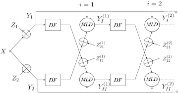
Figure 2: DF-based symmetric cooperation

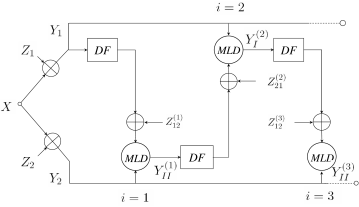
Figure 3: DF-based asymmetric cooperation

IV-C Maximum likelihood detector

The purpose of this section is to present a generalized version of the ML combiner used in [16][17][18]. In these works, the authors assumed a binary phase shift keying modulation at the source and relay, and derived the corresponding ML detector. Reference [16] showed that, under this assumption, the gain provided by the MLD over the MRC can be significant when the relay has a receive SNR close to (or less than) the destination SNR, and it is negligible otherwise. In this paper the reason for extending the MLD of [16][17][18] is twofold:

• we want the receiver to optimally combine the signals it receives whatever the noise level at the relay;

• it also turns out that the MRC does not seem to be suited for combining signals using different constellations and its derivation is not ready, perhaps impossible.

Before providing the signal model used for the derivation of the MLD, we consider a special case in order to clearly explain the idea of compatibility between the modulations used by the source and relay. Assume that $B_{DL}=B$, $B_{C}=\frac{B}{4}$, $K=1$ and the source transmits at the rate of $d=1\ \mathrm{bpcu}$. As the relay has to use the channel twice more often than the source, the relay has to transmit 4 bpcu in order to send at the same coded bit rate as the source. For example, if the source and relay implement the same kind of transmit filters (e.g. a root raised-cosine filter), and the source uses a BPSK modulation, the relay can use a 16-QAM modulation. In this example the MLD has to combine one 16-QAM symbol with four BPSK symbols. In general, the MLD will have to combine $r$ $M_{r}-$ary symbols from the relay with $s$ $M_{s}-$ary symbols from the source, where $r$ and $s$ are linked through the condition of conservation of the coded bit rate between the input and output of the relay: $r\log_{2}M_{r}=s\log_{2}M_{s}\triangleq n$.

Without loss of generality assume $K=1$, consider receiver 1 sends a cooperation signal to receiver 2 and express the signals received by the latter destination:

$$\left\{\begin{array}[]{ccll}Y_{2}^{(1)}&=&X^{(1)}+Z_{2}^{(1)}\\ &\vdots&\\ Y_{2}^{(s)}&=&X^{(s)}+Z_{2}^{(s)}\\ Y_{12}^{(1)}&=&a_{12}\epsilon^{(1)}X_{I}^{(1)}+Z_{12}^{(1)}\\ &\vdots&\\ Y_{12}^{(r)}&=&a_{12}\epsilon^{(r)}X_{I}^{(r)}+Z_{12}^{(r)}\end{array}\right.$$ (21)

where $\forall i\in\{1,...,r\},\ X^{(i)}\in\{x_{1},...,x_{M_{s}}\}$, $\forall i\in\{1,...,r\},\ X_{I}^{(i)}\in\{x_{I,1},...,x_{I,M_{r}}\}$ and the random variables $\epsilon^{(i)}$ model the decoding noise introduced by the relay. For example, when the relay uses a QPSK modulation, $\epsilon^{(i)}\in\{1,e^{j\frac{\pi}{2}},e^{j\pi},e^{j\frac{3\pi}{2}}\}$. Now, in order to express the likelihood at receiver 2, we introduce the following notations: $\underline{Y}_{2}=(Y_{2}^{(1)},...,Y_{2}^{(s)})$, $\underline{Y}_{12}=(Y_{12}^{(1)},...,Y_{12}^{(r)})$, $\underline{b}=(b_{1},...,b_{n})$ denotes the vector of coded bits associated with the ordered vector of symbols $\underline{X}=(X^{(1)},...,X^{(r)})$. We want to express the likelihood $p_{ML}=p(\underline{y}_{2},\underline{y}_{12}\ |\ \underline{b})$. We have

$$p_{ML}=p\left(\underline{y_{2}},\underline{y_{12}}\ |\ \underline{b}\right)\stackrel{{\scriptstyle(a)}}{{=}}p\left(\underline{y}_{2},\underline{y}_{12}\ |\ \underline{x}\right)\\ \stackrel{{\scriptstyle(b)}}{{=}}p\left(\underline{y}_{2}\ |\ \underline{x}\right)\ p\left(\underline{y}_{12}\ |\ \underline{x}\right)$$

where
(a) there is a one-to-one mapping between $\underline{X}$ and $\underline{b}$;
(b) the noises of the downlink and the cooperative channels are independent.

Denoting $N_{2}=n_{2}B_{DL}$, the first term of the product in equation (IV-C) expresses as

$$p\left(\underline{y_{2}}\ |\ \underline{x}\right) = p\left(y_{2}^{(1)},...,y_{2}^{(r)}\ |\ x^{(1)},...,x^{(r)}\right)$$ (22)

$$= \prod_{i=1}^{r}p\left(y_{2}^{(i)}\ |\ x^{(i)}\right)$$

$$= \prod_{i=1}^{r}\frac{1}{\pi N_{2}}\exp\left(-\frac{\left|y_{2}^{(i)}-x^{(i)}\right|^{2}}{N_{2}}\right).$$

By denoting $N_{12}=n_{12}\Delta B$ the second term can be expanded as follows

$$p\left(\underline{y_{12}}\ |\ \underline{x}\right) = p\left(\underline{y_{12}}\ |\ \underline{b}\right)$$ (23)

$$= p\left(y_{12}^{(1)},...,y_{12}^{(s)}\ |\ b_{1},...,b_{n}\right)$$

$$\stackrel{{\scriptstyle(c)}}{{=}} \prod_{i=1}^{s}\ p\left(y_{12}^{(i)}\ |\ b_{(i-1)\log_{2}M_{s}+1},...,b_{i\log_{2}M_{s}}\right)$$

$$= \prod_{i=1}^{s}\ p\left(y_{12}^{(i)}\ |\ x_{I}^{(i)}\right)$$

$$\stackrel{{\scriptstyle(d)}}{{=}} \prod_{i=1}^{s}\ \sum_{j=1}^{M_{s}}\ \mathrm{Pr}\left[\epsilon^{(i)}=\epsilon^{(i)}_{j}\left|x_{I}^{(i)}\right.\right]p\left(y_{12}^{(i)}\ |\ x_{I}^{(i)},\epsilon^{(i)}=\epsilon^{(i)}_{j}\right)$$

$$= \prod_{i=1}^{s}\ \sum_{j=1}^{M_{s}}\ \mathrm{Pr}\left[\epsilon^{(i)}=\epsilon^{(i)}_{j}\left|x_{I}^{(i)}\right.\right]\ \frac{1}{\pi N_{12}}\exp\left(-\frac{\left|y_{12}^{(i)}-\epsilon^{(i)}_{j}x_{I}^{(i)}\right|^{2}}{N_{12}}\right)$$

with
(c) given $x_{I}^{(i)}$, the signal $y_{12}^{(i)}$ is independent of $x_{I}^{(j)}$ for $j\neq i$; remind that $x_{I}^{(i)}$ is associated with $(b_{(i-1)\log_{2}M_{s}+1},...,b_{i\log_{2}M_{s}})$.
(d) is obtained by marginalizing over $\epsilon^{(i)}$.

As in [19], we want to express the log likelihood ratio associated with a given coded bit as a function of the likelihood expressed above. To this end, let us define the sets: $\mathcal{B}_{i}^{(n)}(k)=\{\underline{b}\in\{0,1\}^{n},\ b_{k}=i$ with $i=0$ or $i=1$. The coded bits $b_{k}$ being equiprobable we have:

$$LLR\left(b_{k}\right) \triangleq \frac{p\left(\underline{y}_{2},\underline{y}_{12}\ |\ b_{k}=1\right)}{p\left(\underline{y}_{2},\underline{y}_{12}\ |\ b_{k}=0\right)}$$ (24)

$$= \frac{\displaystyle{\sum_{\underline{b}\in\mathcal{B}^{(n)}_{1}(k)}}p\left(\underline{y}_{2},\underline{y}_{12}\ |\ \underline{b}\right)}{\displaystyle{\sum_{\underline{b}\in\mathcal{B}^{(n)}_{0}(k)}}p\left(\underline{y}_{2},\underline{y}_{12}\ |\ \underline{b}\right)}$$

$$= \frac{\displaystyle{\sum_{\underline{x}\in\mathcal{X}^{k}_{1}}}\ p\left(\underline{y}_{2},\underline{y}_{12}\ |\ \underline{x}\right)}{\displaystyle{\sum_{\underline{x}\in\mathcal{X}^{k}_{0}}}\ p\left(\underline{y}_{2},\underline{y}_{12}\ |\ \underline{x}\right)}.$$

This LLR can be either used to make a decision on the bits sent by the source or re-used as a soft information by a stage following the combiner. As we restrict our attention to the raw BER for our performance study, we will not consider the way of using this LLR by the channel decoder for example.

V Experimental analysis

V-A System performance criteria

In order to compare the different cooperation schemes, suited system performance criteria have to be selected. By way of an example, if we fix the information rate/spectral efficiency at the transmitter and obtain the pair of BERs $(BER_{1},BER_{2})$ for the coding scheme $\mathcal{C}$ and $(BER_{1}^{\prime},BER_{2}^{\prime})$ for the coding scheme $\mathcal{C}^{\prime}$, with $BER_{1}<BER_{1}^{\prime}$ and $BER_{2}>BER_{2}^{\prime}$, one cannot easily conclude, which shows the importance of using a system performance metric. From now on, we will denote by $K$ the number of cooperation exchanges with $K$ equals $K_{a}$ or $2K_{s}$ depending on the cooperation scheme. In order to compare the different cooperation strategies, we propose four performance criteria (eq. (25)-(28)). All the performance criteria can be used to evaluate the performance of the system for both relaying protocols but the performance criterion 1) is less meaningful for the DF protocol since the channel input is not Gaussian in our context.

1. $$R_{AF}^{(K)}=B_{DL}\min\left\{\log\left(1+\rho_{I}^{(K)}\right),\log\left(1+\rho_{II}^{(K)}\right)\right\}$$ (25)

   where $\rho_{I}^{(K)}$, $\rho_{II}^{(K)}$ are the SNRs at the end of the cooperation procedure. One can notice that $R_{AF}^{(K)}$ represents the maximum information rate possible for a reliable transmission achieved by the AF-based cooperation schemes and a Gaussian channel input.

2. $$P_{e,max}^{(K)}=\max\left\{P_{e,I}^{(K)},P_{e,II}^{(K)}\right\}$$ (26)

   where $P_{e,I}^{(K)}$ and $P_{e,II}^{(K)}$ are the raw BERs at the combiner (i.e. the MRC for the AF protocol, the MLD for the DF protocol) outputs at the end of the cooperation procedure. This criterion is useful in a broadcasting system for which one wants every user to have a minimum transmission quality, which requires $P_{e,max}^{(K)}\leq P_{e,0}$ where $P_{e,0}$ is the minimum quality target.

3. $$P_{e,sum}^{(K)}=P_{e,I}^{(K)}+P_{e,II}^{(K)}.$$ (27)

   This criterion gives an image of the average transmission quality of the broadcasting system and serves as an upper bound for the performance criterion given just below. Although this criterion does not translate the variance of the qualities of the different communications it has the merit to be simple, which is the reason why many works assumed this criterion (see e.g. [20][21]).

4. $$P_{e,max}^{(K)}\leq P_{e,sys}^{(K)}\leq P_{e,sum}^{(K)}.$$ (28)

   The quantity $P_{e,sys}^{(K)}$ is the system probability of errors $P_{e,sys}^{(K)}$, which is defined as the probability that receiver 1 or (inclusive or) receiver 2 makes a decision error. This probability is generally not easy to explicit but can be bounded by using the criteria (26) and (27). As a comment, note that the Shannon capacity of the channel under consideration is precisely defined with respect to the system error probability, which means that communicating at a rate less than the capacity insures the existence of a code such that $P_{e,sys}^{K^{*}}\rightarrow 0$. It is therefore the criterion to be considered to assess the sub-optimality of a given channel coding scheme in the CBC w.r.t its Shannon limit.

V-B Simulation results for the AF protocol

On all figures $R^{K}_{AF}$ and $R^{K}_{AF}-DL$ denote the achievable rates with the strategy $\mathcal{S}_{1}$ and the strategy $\mathcal{S}_{2}$ respectively.

Asymmetric cooperation: Which user should start cooperating first?
For both strategies $\mathcal{S}_{1}$ and $\mathcal{S}_{2}$, Figure 4 represents the plane $(n_{1},n_{2})$ with linear scales: $n_{1}\in[10^{-2},10^{2}]$, $n_{2}\in[10^{-2},10^{2}]$. For different ratios
$\frac{P_{12}}{P_{21}}\in\{-30\ \mathrm{dB},-10\ \mathrm{dB},0\ \mathrm{dB},10\ \mathrm{dB},30\ \mathrm{dB}\}$. The different curves delimit the decision regions that allow us to determine the best cooperation order in terms of information rate for the five values of the ratio $\frac{P_{12}}{P_{21}}$. When the pair $(n_{1},n_{2})$ is above the line, receiver 1 has to start first and conversely. We see that both the DL and cooperation SNRs have to be considered to optimize the overall performance. In a cellular system for instance, the cooperation powers can be quite close (a given fraction of the mobile transmit power), which would make the cooperation order less critical.

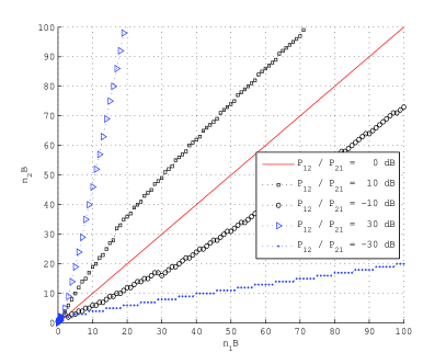
Figure 4: Decision regions: who starts cooperating first?

Comparison between the strategies $\mathcal{S}_{1}$ and $\mathcal{S}_{2}$.

We first consider the case of a constant the global bandwidth. We look at three different SNR scenarios:
$(\frac{P}{n_{1}B},\frac{P}{n_{2}B},\frac{P_{12}}{n_{12}B},\frac{P_{21}}{n_{21}B},)=(10\ \mathrm{dB},0\ \mathrm{dB},30\ \mathrm{dB},30\ \mathrm{dB})$, $(\frac{P}{n_{1}B},\frac{P}{n_{2}B},\frac{P_{12}}{n_{12}B},\frac{P_{21}}{n_{21}B},)=(-1\ \mathrm{dB},-4\ \mathrm{dB},30\ \mathrm{dB},30\ \mathrm{dB})$ and $(\frac{P}{n_{1}B},\frac{P}{n_{2}B},\frac{P_{12}}{n_{12}B},\frac{P_{21}}{n_{21}B},)=(10\ \mathrm{dB},0\ \mathrm{dB},15\ \mathrm{dB},15\ \mathrm{dB})$. Figure 5 and 5 represent the performances of both strategies $\mathcal{S}_{1}$ and $\mathcal{S}_{2}$ where the asymmetric cooperation is considered. Both strategies have approximately the same performance but the strategy $\mathcal{S}_{2}$ can perform better than the strategy $\mathcal{S}_{1}$ for great values of $K$ ($K>2$, see Figure 5). Since the optimum is obtained in general at low values of $K$ ($K\leq 2$), we can conclude that both strategies $\mathcal{S}_{1}$ and $\mathcal{S}_{2}$ have similar performances in asymmetric cooperation. We have also observed that this conclusion remains valid when the symmetric cooperation is considered.

Now, we consider the case where the DL bandwidth is constant. In Figure 6 can consider two different scenarios for the $\mathcal{S}_{2}$ for the asymmetric cooperation case:
$(\frac{P}{n_{1}B},\frac{P}{n_{2}B},\frac{P_{12}}{n_{12}B},\frac{P_{21}}{n_{21}B})=(10\ \mathrm{dB},10\ \mathrm{dB},30\ \mathrm{dB},30\ \mathrm{dB})$ and $(\frac{P}{n_{1}B},\frac{P}{n_{2}B},\frac{P_{12}}{n_{12}B},\frac{P_{21}}{n_{21}B},)=(10\ \mathrm{dB},10\ \mathrm{dB},16\ \mathrm{dB},16\ \mathrm{dB})$. We observe that the SIMO bound is rapidly attained ($K=2$). Also we have observed that, for the strategy $\mathcal{S}_{2}$, the symmetric and asymmetric cooperations perform the same. This means that for the symmetric case also the SIMO bound is attained for $K_{s}=1$. In the following paragraph we will compare these results with the results obtained with the stategy $\mathcal{S}_{1}$ in the same setup ( DL bandwidth constant).

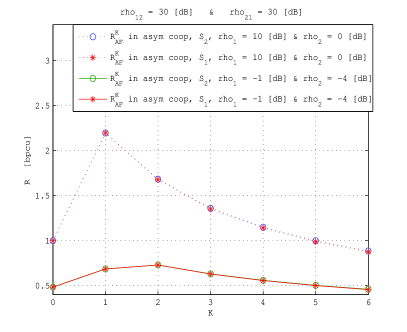
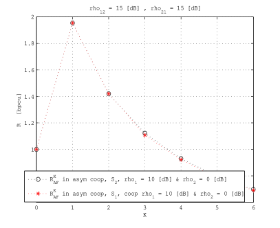
Figure 5: Achievable rate vs number of cooperation exchanges for both strategies $\mathcal{S}_{1}$ and $\mathcal{S}_{2}$ when the total bandwidth is fixed at high cooperative regime (a)  or medium cooperative regime  (b).

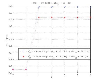
Figure 6: Achievable rate vs number of cooperation exchanges for the strategy $\mathcal{S}_{2}$ when the downlink bandwidth is fixed for medium and high cooperative regimes.

Asymmetric cooperation vs symmetric cooperation for the strategy $\mathcal{S}_{1}$. First we assume the total bandwidth to be limited. Figure 7 represents the information rate as a function of the number of cooperation exchanges for the asymmetric and symmetric cases for two different scenarios:
$(\frac{P}{n_{1}B},\frac{P}{n_{2}B},\frac{P_{12}}{n_{12}B},\frac{P_{21}}{n_{21}B},)=(10\ \mathrm{dB},0\ \mathrm{dB},30\ \mathrm{dB},30\ \mathrm{dB})$ and $(\frac{P}{n_{1}B},\frac{P}{n_{2}B},\frac{P_{12}}{n_{12}B},\frac{P_{21}}{n_{21}B},)=(-1\ \mathrm{dB},-4\ \mathrm{dB},30\ \mathrm{dB},30\ \mathrm{dB})$. It can be seen that the rate always decreases for $K\geq 2$. This is not surprising since a system with $K>2$ is a special case of the system for which $K=2$. However note that the system with $K=2$ is not a special of the system $K=0$ or $K=1$, which means that cooperating can compensate for the performance loss due do orthogonalizing the DL channel. We also see that the asymmetric system performs better than its symmetric counterpart. We observed from other simulations not presented here that most of the cooperation benefits are captured with one cooperation exchange. In contrast with the discrete CBC with a conference channel [5][9][10] we see that the performance can decrease with $K$. Now we look at two scenarios where the downlink bandwidth is fixed (Figure 7):
$(\frac{P}{n_{1}B},\frac{P}{n_{2}B},\frac{P_{12}}{n_{12}B},\frac{P_{21}}{n_{21}B})=(10\ \mathrm{dB},10\ \mathrm{dB},30\ \mathrm{dB},30\ \mathrm{dB})$ and $(\frac{P}{n_{1}B},\frac{P}{n_{2}B},\frac{P_{12}}{n_{12}B},\frac{P_{21}}{n_{21}B},)=(10\ \mathrm{dB},10\ \mathrm{dB},16\ \mathrm{dB},16\ \mathrm{dB})$. We see that in the high cooperation regime the SIMO bound is rapidly attained; that is for $K=2$. When less cooperation powers are available the performance still decreases with $K$. This time this is not due to the orthogonalization loss but to the fact that the cooperation power per exchange decreases in $\sim\frac{1}{K}$ whereas the gain brought by increasing the number of recombinations increases slowly. Note that now the symmetric system performs better than the asymmetric one because nothing is lost in terms of bandwidth by increasing $K$ (while for the case where the total bandwidth was limited the DL bandwidth was decreasing according to propositions III.2 and III.3).

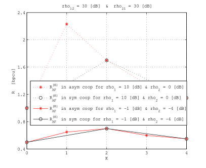
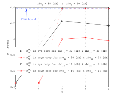
Figure 7: Achievable rate vs number of cooperation exchanges for the strategy $\mathcal{S}_{1}$ when the total bandwidth is fixed  (a)  or when the downlink bandwidth is fixed  (b).

Comparing the results of the strategies $\mathcal{S}_{1}$ and $\mathcal{S}_{2}$ when the DL bandwidth is constant ( Figures 7 and 6), we have observed that both strategies perform identically for the symmetric cooperation when there is enough power available for the cooperation (high cooperative regime). If the cooperative power is reduced, the strategy $\mathcal{S}_{2}$ will perform better than the strategy $\mathcal{S}_{1}$, starting from $K_{s}=2$ (equivalent to $K=2$). In fact, using the strategy $\mathcal{S}_{1}$, during the second exchange round, the receiver acting as relay is waisting a part of the limited available power to send to the other receiver a signal that it has already received on the downlink channel. Thus, the expected power gain from the cooperation is limited w.r.t. the strategy $\mathcal{S}_{2}$, where the receiver acting as relay uses all of the available power to send the signal needed to increase the equivalent SNR. However, since the optimal performance is obtained for $K_{s}=1$, we can conclude that both strategies have the same performance for symmetric cooperation case.

For the strategy $\mathcal{S}_{2}$ the symmetric and asymmetric cooperation schemes perform identically. This is also the case for the strategy $\mathcal{S}_{1}$ but only when the high cooperative regime is assumed. For the strategy $\mathcal{S}_{2}$, the achievable rates remain constant after $K_{s}=1$, whatever the cooperation power level. For the strategy $\mathcal{S}_{1}$, if the cooperation powers are limited, the symmetric cooperation case outperforms its asymmetric counterpart. Also, for the asymmetric cooperation with limited cooperation powers, the strategy $\mathcal{S}_{2}$ performs better than the strategy $\mathcal{S}_{1}$ even at the optimum number of cooperation rounds $K^{*}$.

Influence of the performance criterion and BER analysis.

In the simulations results presented so far we have implicitly assumed the channel input and relay outputs to be Gaussian, which allowed us to provide an achievable rate for the channel under investigation. In the following part of the section we will assume finite modulations (QAM modulations). It turns out that the observations made for the information theoretic transmission rate are generally confirmed by the raw BER analysis and under the QAM assumption. This fact is illustrated in Figures 8 and 8. In both figures the asymmetric cooperation case and the strategy $\mathcal{S}_{1}$ is assumed. Also, the first figure corresponds to Assumption $\mathcal{H}_{1}$ while the second one is based on Assumption $\mathcal{H}_{1}$. The system BER is minimized for $K=1$ or $K=2$ whatever the assumption on spectral resources.

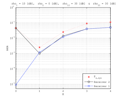
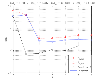
Figure 8: System BER vs number of cooperation exchanges for strategy $\mathcal{S}_{1}$ and the asymmetric cooperation case when the total bandwidth is fixed  (a)  or when the downlink bandwidth is fixed  (b).

V-C Simulation results for the DF protocol

In the case of the DF protocol, we always assume that only the downlink bandwidth is fixed. As a consequence the total bandwidth increases with $K$ (see Assumption $\mathcal{H}_{2}$ in sec. II).

Asymmetric cooperation vs symmetric cooperation.

We always assume QAM modulations at the source and relays and we do take into account the possible presence of channel coders at the source and relay. We consider two different scenarios: a high cooperative regime with $(\frac{P}{n_{1}B},\frac{P}{n_{2}B},\frac{P_{12}}{n_{12}B},\frac{P_{21}}{n_{21}B},)=(7\ \mathrm{dB},3\ \mathrm{dB},30\ \mathrm{dB},30\ \mathrm{dB})$ and a low cooperative regime with $(\frac{P}{n_{1}B},\frac{P}{n_{2}B},\frac{P_{12}}{n_{12}B},\frac{P_{21}}{n_{21}B},)=(7\ \mathrm{dB},3\ \mathrm{dB},2\ \mathrm{dB},2\ \mathrm{dB})$. We use a 4-QAM modulation for any transmission at the source and at the relay. We only consider the uncoded case but the performance analysis can be extended to coded case, at least for hard input decoders. We assume that receiver 1 starts sending a cooperation in the asymmetric cooperation case. Figures 9 and 9 show the system performance as a function of the number of cooperation exchanges for performance criteria 2. and 4. respectively. In the low cooperation regime, symmetric and asymmetric cooperations perform similarly. In the high cooperation regime, the asymmetric cooperation performs slightly better for $P_{e,sys}$ and conversely for $P_{e,max}$. Other simulations, which will not provided here for keeping the number of figures reasonable, show that the performance of asymmetric cooperation is generally better than that of its symmetric counterpart, whatever the performance criterion under consideration. In contrast with the AF case it is more difficult to determine analytically which receiver has to start cooperation in the first place. This means that, in practice, this information has to be sent to the receivers. Otherwise, the symmetric cooperation has to be used.

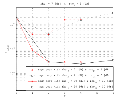
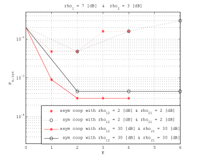
Figure 9: Performance vs number of cooperation exchanges in term of $P_{e,sys}$  (a) and $P_{e,max}$  (b).

Asymmetric cooperation: influence of both number of cooperation exchanges and combining scheme.

Figures 10 and 10 show the performance for receiver 1 and 2, the system performance in the low and high cooperation regimes respectively as defined previously. Although the system bandwidth increases with $K$, we see that the system performance is maximum (low cooperation regime) or reaches a floor (high cooperation regime) for two cooperation exchanges. There are at least three reasons for this. First of all, the gain provided by an additional cooperation round decreases with $K$. Second, the cooperation power per exchange also decreases with $K$. In addition, in order to derive the MLD, we have made the simplifying assumption that the decoding errors and receive noise at each receiver are independent, which is perfectly true for $K\leq 2$. In Figure 10 we also observe the impact of the derived MLD on system performance. We compare the DF protocol associated to MLD with the AF protocol associated to the MRC in terms of the system and individual receivers performance, and we observe that the use of the MRC limits the expected performance gain since this combiner does not take into account the eventual decoding made at the receivers unlike the MLD. The observations are similar to those in [16].

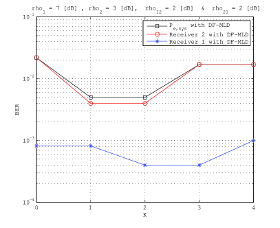
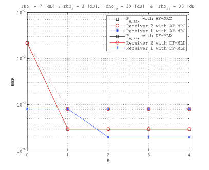
Figure 10: Performance for the asymmetric cooperation vs number of cooperation exchanges in low cooperative regime  (a)  and high cooperative regime  (b).

V-D Comparison between the AF protocol (strategy $\mathcal{S}_{1}$) and the DF protocol.

We consider the case where only the downlink bandwidth is fixed. We look at the following SNR scenario: $(\frac{P}{n_{1}B},\frac{P}{n_{2}B},\frac{P_{12}}{n_{12}B},\frac{P_{21}}{n_{21}B},)=(7\ \mathrm{dB},3\ \mathrm{dB},30\ \mathrm{dB},30\ \mathrm{dB})$ and $(\frac{P}{n_{1}B},\frac{P}{n_{2}B},\frac{P_{12}}{n_{12}B},\frac{P_{21}}{n_{21}B},)=(7\ \mathrm{dB},3\ \mathrm{dB},2\ \mathrm{dB},2\ \mathrm{dB})$. Figure 11 represent the BER performance obtained with the AF protocol (strategy $\mathcal{S}_{1}$) associated with the MRC and the DF protocol associated with the MLD. We observe the impact of the hard decision with the DF protocol which results in a performance loss in comparison to the AF protocol. This is due to the fact that the receiver acting as the sender does not decode perfectly the message. If one receiver can succeed to decode the message with only the downlink signal, the DF protocol would perform better than the AF one (see [16] for the same analysis on the relay channel) and the optimal number of cooperative exchanges will obviously be equal to $K^{*}=1$.

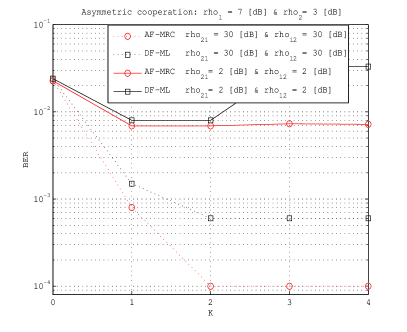
Figure 11: maximum BER  (max$\{BER_{1},BER_{2}\}$)  at the receivers for the AF protocol ($\mathcal{S}_{1}$) with MRC and DF protocol with MLD

VI Conclusions

In this paper we treated four main issues inherent to the bidirectional CBC with a single common message when power and spectral resources are taken into account, which cannot be considered through the discrete approach [5, 9, 10]. This study was made for a simplified scenario where scalar relaying protocols are assumed and channel coding/decoding are not exploited (note however that one of the main practical advantages of this approach is that the extra decoding delay induced by cooperation is relatively small). Although we have made these simplifying assumptions, our approach still captures the main implementation issues posed by the bidirectional cooperation. The observations made in this paper could be refined and used to introduce cooperation in systems like the DVB or DVB-H systems. Here are a few key observations we have made.

Concerning the way of combining the signals at the receiver we have seen that the MRC is the optimum combiner whatever the number of cooperation rounds when the AF protocol is used. For the DF protocol we have not only seen that an ML detector is useful since it can compensate for the decoding noise introduced by the other receiver but also that it is necessary to combine signals with different constellations, which is likely to happen in practice if the downlink and cooperation channels have different bandwidths. Additionally the choice between sending the downlink signal or the combiner output as a cooperation signal does not seem to be critical for the AF protocol but the second solution complicates the derivation of the ML detector.

Number of cooperation rounds. By assuming the system total bandwidth and then the downlink bandwidth to be constant, we have seen that the system performance does not increase for more than two cooperation rounds ($K^{*}\in\{0,1,2\}$), in contrast with [5, 9] for discrete channels. We have shown for the AF protocol that the equivalent SNR is strictly constant for $K\geq 2$ for the strategy $\mathcal{S}_{2}$ and is almost constant or reaches its maximum for $K=1,2$ or marginally for $3$ with the strategy $\mathcal{S}_{1}$.

Asymmetric/symmetric cooperation: when the system bandwidth is fixed the asymmetric cooperation has the advantage to contain the case $K=1$ for which the best performance is generally achieved. Indeed as the bandwidth decreases linearly with $K$ but only logarithmically with the SNR, higher values of $K$ generally lead to suboptimum performance. This is the main reason why the asymmetric cooperation is preferable to the symmetric cooperation. When the downlink bandwith is fixed, the best performance can be achieved for $K=2$ typically. In this case, the asymmetric cooperation suffers of a correlation effect which reduces the cooperation gain w.r.t. the symmetric case. Additionally for $K\geq 2$ the user who starts sending the cooperation signal has to be selected. The influence of the available cooperation powers and noise levels at the receiver on the best order was assessed and shown to be not negligible. In fading channels, this order should therefore be chosen adaptively, which is a further drawback of the asymmetric cooperation if $K^{*}\geq 2$. On the other hand, if most of the performance gain could be captured by one cooperation round ($K^{*}=1$), the asymmetric case is the best choice.

VII Appendix

VII-A Conservation of the MI for the MRC

Proof: We want to prove that $I(X;Y_{II}^{(i)})=I(X;Y_{II}^{(i-1)},Y_{12}^{(i)})$. Using the same notations as in Section III.A. and B. we obtain that:

$$I(X;Y_{II}^{(i)})=\log\left[1+\frac{\left|w_{12}^{(i)}a_{12}^{(i)}\alpha_{I}^{(i-1)}+w_{2}^{(i)}\alpha_{II}^{(i-1)}\right|^{2}P}{\left|w_{12}^{(i)}\right|^{2}\left((a_{12}^{(i)})^{2}N_{I}^{(i-1)}+N_{12}^{(i)}\right)+\left|w_{2}^{(i)}\right|^{2}N_{II}^{(i-1)}+w_{2}^{(i)}w_{12}^{(i)}a_{12}^{(i)}(e^{(i-1)}+e^{(i-1),*})}\right]$$ (29)

Now, by replacing the MRC weights given in Proposition 1, we further have:

$$I(X;Y_{II}^{(i)})=\log\left[1+\frac{S_{2}^{(i)}}{T_{2}^{(i)}}\right]$$ (30)

where $S_{2}^{(i)}$ and $T_{2}^{(i)}$ are given by the following expressions:

$$S_{2}^{(i)}=\left((\alpha_{II}^{(i-1)})^{2}\left((a_{12}^{(i)})^{2}N_{I}^{(i-1)}+N_{12}^{(i)}\right)+\alpha_{I}^{(i-1)}a_{12}^{(i)}N_{II}^{(i-1)}-(a_{12}^{(i-1)})^{2}\alpha_{I}^{(i-1)}\alpha_{II}^{(i-1)}(e^{(i-1)}+e^{(i-1),*})\right)P$$ (31)

$$T_{2}^{(i)}=N_{II}^{(i-1)}\left((a_{12}^{(i)})^{2}N_{I}^{(i-1)}+N_{12}^{(i)}\right)-a_{12}^{(i)}|e^{(i-1)}|^{2}$$ (32)

On the other hand we have

$$\begin{array}[]{ccl}I(X;Y_{II}^{(i-1)},Y_{12}^{(i)})&=&I(X;(\alpha_{II}^{(i-1)}X+Z_{II}^{(i-1)}),(a_{12}^{(i)}\alpha_{I}^{(i-1)}X+a_{12}^{(i)}Z_{I}^{(i-1)}+Z_{12}^{(i)}))\\ &=&\log\left[1+\frac{\tilde{S}_{2}^{(i)}}{\tilde{T}_{2}^{(i)}}\right].\end{array}$$ (33)

We see that $\tilde{S}_{2}^{(i)}=S_{2}^{(i)}$ and $\tilde{T}_{2}^{(i)}=S_{2}^{(i)}$, which concludes the proof

VII-B Proof of theorem III.1

Here we show the result obtained for the equivalent SNR in Theorem III.1. At receiver 2, for the iteration $i\in\{1,...,K\}$, the signal at the MRC output is denoted by $Y_{II}^{(i)}=\alpha_{II}^{(i)}X+Z_{II}^{(i)}$. The equivalent SNR $\rho_{II}^{(i)}$ in $Y_{II}^{(i)}$ expresses as $\rho_{II}^{(i)}\triangleq\frac{E\left|\alpha_{II}^{(i)}X\right|^{2}}{E\left|Z_{II}^{(i)}\right|^{2}}=\frac{\mathcal{S}^{(i)}}{\mathcal{T}^{(i)}}$ with

$$\mathcal{S}^{(i)} = E\left|\alpha_{II}^{(i)}X\right|^{2}$$

$$= \left[w_{12}^{(i)}a_{12}^{(i)}\alpha_{I}^{(i-1)}+w_{2}^{(i)}\alpha_{II}^{(i-1)}\right]^{2}P$$

$$= \left[\left(a_{12}^{(i)}\alpha_{I}^{(i-1)}N_{II}^{(i-1)}-a_{12}^{(i)}\alpha_{II}^{(i-1)}e^{(i-1)}\right)a_{12}^{(i)}\alpha_{I}^{(i-1)}\right.$$

$$+\left.\left([\left(a_{12}^{(i)}\right)^{2}N_{I}^{(i-1)}+N_{12}^{(i)}]\alpha_{II}^{(i-1)}-\left(a_{12}^{(i)}\right)^{2}\alpha_{I}^{(i-1)}e^{(i-1)}\right)\alpha_{II}^{(i-1)}\right]^{2}P$$

$$= \left[\left(\alpha_{I}^{(i-1)}\alpha_{II}^{(i-1)}\right)^{2}PN_{12}+\left(\alpha_{I}^{(i-1)}\right)^{2}N_{II}^{(i-1)}P_{12}+\left(\alpha_{II}^{(i-1)}\right)^{2}N_{I}^{(i-1)}P_{12}-\alpha_{I}^{(i-1)}\alpha_{II}^{(i-1)}P_{12}\left(e^{(i-1)}+e^{(i-1),*}\right)\right.$$

$$+\left.\left(\alpha_{II}^{(i-1)}\right)^{2}N_{I}^{(i-1)}N_{12}\right]$$

$$\cdot\underbrace{\left[\left(a_{12}^{(i)}\alpha_{I}^{(i-1)}\right)^{2}N_{II}^{(i-1)}+\left(a_{12}^{(i)}\alpha_{II}^{(i-1)}\right)^{2}N_{I}^{(i-1)}+\left(\alpha_{II}^{(i-1)}\right)^{2}N_{12}-\left(a_{12}^{(i)}\right)^{2}\alpha_{I}^{(i-1)}\alpha_{II}^{(i-1)}\left(e^{(i-1)}+e^{(i-1),*}\right)\right]}_{\mathcal{C}}P$$

and,

$$\mathcal{T}^{(i)} = E\left|Z_{II}^{(i)}\right|^{2}$$

$$= \left(w_{12}^{(i)}a_{12}^{(i)}\right))^{2}N_{I}^{(i-1)}+\left(w_{12}^{(i)}\right)^{2}N_{12}^{(i)}+\left(w_{2}^{(i)}\right)^{2}N_{II}^{(i-1)}+2w_{12}^{(i)}w_{2}^{(i)}\left(e^{(i-1)}+e^{(i-1),*}\right)$$

$$= \left(a_{12}^{(i)}\alpha_{I}^{(i-1)}N_{II}^{(i-1)}-a_{12}^{(i)}\alpha_{II}^{(i-1)}e^{(i-1)}\right)^{2}\left(\left(a_{12}^{(i)}\right)^{2}N_{I}^{(i-1)}+N_{12}^{(i)}\right)$$

$$+\left(\left[(a_{12}^{(i)})^{2}N_{I}^{(i-1)}+N_{12}^{(i)}\right]\alpha_{II}^{(i-1)}-(a_{12}^{(i)})^{2}\alpha_{I}^{(i-1)}e^{(i-1)}\right)^{2}N_{II}^{(i-1)}$$

$$+2\left([(a_{12}^{(i)})^{2}N_{I}^{(i-1)}+N_{12}^{(i)}]\alpha_{II}^{(i-1)}-(a_{12}^{(i)})^{2}\alpha_{I}^{(i-1)}e^{(i-1)}\right)$$

$$\hskip 11.38092pt\cdot\left(a_{12}^{(i)}\alpha_{I}^{(i-1)}N_{II}^{(i-1)}-a_{12}^{(i)}\alpha_{II}^{(i-1)}e^{(i-1)}\right)\left(e^{(i-1)}+e^{(i-1),*}\right)$$

$$= \left[P_{12}e^{(i-1)}e^{(i-1),*}-\left(\alpha_{I}^{(i-1)}\right)^{2}PN_{II}^{(i-1)}N_{12}-N_{I}^{(i-1)}N_{II}^{(i-1)}\left(P_{12}+N_{12}\right)\right]$$

$$\cdot\underbrace{\left[\left(a_{12}^{(i)}\alpha_{I}^{(i-1)}\right)^{2}N_{II}^{(i-1)}+\left(a_{12}^{(i)}\alpha_{II}^{(i-1)}\right)^{2}N_{I}^{(i-1)}+\left(\alpha_{II}^{(i-1)}\right)^{2}N_{12}-\left(a_{12}^{(i)}\right)^{2}\alpha_{I}^{(i-1)}\alpha_{II}^{(i-1)}\left(e^{(i-1)}+e^{(i-1),*}\right)\right]}_{\mathcal{C}}$$

After simplification w.r.t. the common factor $\mathcal{C}$, we obtain $\rho_{II}^{(i)}=\frac{\mathcal{S}_{I}^{(i)}}{\mathcal{T}_{I}^{(i)}}$ with

$$\begin{array}[]{ccl}\mathcal{S}_{I}^{(i)}&=&\left[\left(\alpha_{I}^{(i-1)}\alpha_{II}^{(i-1)}\right)^{2}PN_{12}+\left(\alpha_{I}^{(i-1)}\right)^{2}N_{II}^{(i-1)}P_{12}+\left(\alpha_{II}^{(i-1)}\right)^{2}N_{I}^{(i-1)}P_{12}-\alpha_{I}^{(i-1)}\alpha_{II}^{(i-1)}P_{12}\left(e^{(i-1)}+e^{(i-1),*}\right)\right.\\ &&\left.+\left(\alpha_{II}^{(i-1)}\right)^{2}N_{I}^{(i-1)}N_{12}\right]P\\ \\ \mathcal{T}_{I}^{(i)}&=&\left[P_{12}e^{(i-1)}e^{(i-1),*}-\left(\alpha_{I}^{(i-1)}\right)^{2}PN_{II}^{(i-1)}N_{12}-N_{I}^{(i-1)}N_{II}^{(i-1)}\left(P_{12}+N_{12}\right)\right]\end{array}$$

Then, by multiplying both the numerator and the denominator of $\rho_{II}^{(i)}$ by the factor $\displaystyle{\frac{\rho_{I}^{(i-1)}\rho_{II}^{(i-1)}}{PN_{12}}}$, we obtain $\rho_{II}^{(i)}=\displaystyle{\frac{\mathcal{S}_{II}^{(i)}}{\mathcal{T}_{II}^{(i)}}}$ with

$$\begin{array}[]{ccl}\mathcal{S}_{II}^{(i)}&=&\displaystyle{\alpha_{I}^{(i-1)}\alpha_{II}^{(i-1)}\left(e^{(i-1)}+e^{(i-1),*}\right)\rho_{I}^{(i-1)}\rho_{II}^{(i-1)}\rho_{12}}\displaystyle{-\left(\alpha_{I}^{(i-1)}\alpha_{II}^{(i-1)}\right)^{2}P\left[\rho_{II}^{(i-1)}\left(1+\rho_{I}^{(i-1)}\right)\right.}\\ &&\displaystyle{+\left.\rho_{12}\left(\rho_{I}^{(i-1)}+\rho_{II}^{(i-1)}\right)\right]}\\ \\ \mathcal{T}_{II}^{(i)}&=&\displaystyle{\frac{e^{(i-1)}e^{(i-1),*}}{P}\rho_{I}^{(i-1)}\rho_{II}^{(i-1)}\rho_{12}}\displaystyle{-\left(\alpha_{I}^{(i-1)}\alpha_{II}^{(i-1)}\right)^{2}P\left(1+\rho_{12}\right)}-\displaystyle{\left(\alpha_{I}^{(i-1)}\right)^{2}N_{II}^{(i-1)}\rho_{I}^{(i-1)}\rho_{II}^{(i-1)}}.\end{array}$$ (34)

VII-C Proof of Proposition III.2: symmetric cooperation

Here we only show how to obtain the MRC weights, and this for receiver 2. The signal coefficients and equivalent noises can be derived from the equivalent signal expressions.
At receiver 2, at the iteration $i$, the signals available at the combiner inputs are

$$\left\{\begin{array}[]{ccll}Y_{12}^{(i)}&=&a_{12}^{(i)}Y_{I}^{(i-1)}+Z_{12}^{(i)}=a_{12}^{(i)}\alpha_{I}^{(i-1)}X+(a_{12}^{(i)}Z_{I}^{(i-1)}+Z_{12}^{(i)})\\ Y_{II}^{(i-1)}&=&\alpha_{II}^{(i-1)}X+Z_{II}^{(i-1)}\\ \end{array}\right.$$ (37)

Denote by $\boldsymbol{w}^{(i)}=(w_{12}^{(i)},w_{2}^{(i)})^{t}$ the optimal weight vector. For the maximum ratio combiner, $\boldsymbol{w}^{(i)}$ is given by the following expression:

$$\boldsymbol{w}^{(i)}={\boldsymbol{R}_{zz}^{(i)}}^{-1}\cdot\boldsymbol{h}^{*}$$ (38)

where $\boldsymbol{R}_{zz}^{(i)}$ is the covariance matrix between the equivalent noises $(a_{12}^{(i)}Z_{I}^{(i-1)}+Z_{12}^{(i)})$ and $Z_{II}^{(i-1)}$ with

$$\left\{\begin{array}[]{ccc}Z_{I}^{(i-1)}&=&w_{21}^{(i-1)}a_{21}^{(i-1)}Z_{II}^{(i-1)}+w_{21}^{(i-1)}Z_{21}^{(i-1)}+w_{1}^{(i-1)}Z_{I}^{(i-2)}\\ Z_{II}^{(i-1)}&=&w_{12}^{(i-1)}a_{12}^{(i-1)}Z_{I}^{(i-2)}+w_{12}^{(i-1)}Z_{12}^{(i-1)}+w_{2}^{(i-1)}Z_{II}^{(i-2)}.\end{array}\right.$$

and $\boldsymbol{h}$ is the useful signal coefficients vector given by $\boldsymbol{h}=(a_{12}^{(i)}\alpha_{I}^{(i-1)},\alpha_{II}^{(i-1)})^{t}$ with $\alpha_{I}^{(i-1)}$ and $\alpha_{II}^{(i-1)}$ obtained from the following recursive formula

$$\left\{\begin{array}[]{ccl}\alpha_{I}^{(i)}&=&w_{21}^{(i)}a_{21}^{(i)}\alpha_{II}^{(i-1)}+w_{1}^{(i)}\alpha_{I}^{(i-1)}\\ \alpha_{II}^{(i)}&=&w_{12}^{(i)}a_{12}^{(i)}\alpha_{I}^{(i-1)}+w_{2}^{(i)}\alpha_{II}^{(i-1)}.\end{array}\right.$$ (39)

Therefore we find that

$$\boldsymbol{R}_{zz}^{(i)}=\left[\begin{array}[]{ccc}\left(a_{12}^{(i)}\right)^{2}N_{I}^{(i-1)}+N_{12}^{(i)}&&a_{12}^{(i)}e^{(i-1)}\\ a_{12}^{(i)}e^{(i-1),*}&&N_{II}^{(i-1)}\end{array}\right]$$ (42)

and

$${\boldsymbol{R}_{zz}^{(i)}}^{-1}=\frac{1}{\left[\left(a_{12}^{(i)}\right)^{2}N_{I}^{(i-1)}+N_{12}^{(i)}\right]N_{II}^{(i-1)}-|e^{(i-1)}|^{2}}\left[\begin{array}[]{ccc}N_{II}^{(i-1)}&&-a_{12}^{(i)}e^{(i-1)}\\ -a_{12}^{(i)}e^{(i-1),*}&&\left(a_{12}^{(i)}\right)^{2}N_{I}^{(i-1)}+N_{12}^{(i)}\end{array}\right]$$ (45)

where $e^{(i-1)}\triangleq E\left[Z_{I}^{(i-1)}Z_{II}^{(i-1),*}\right]$.
Finally we obtain

$$\left\{\begin{array}[]{ccl}w_{12}^{(i)}&=&a_{12}^{(i)}\alpha_{I}^{(i-1)}N_{II}^{(i-1)}-a_{12}^{(i)}\alpha_{II}^{(i-1)}e^{(i-1)}\\ w_{2}^{(i)}&=&\left[(a_{12}^{(i)})^{2}N_{I}^{(i-1)}+N_{12}^{(i)}\right]\alpha_{II}^{(i-1)}-(a_{12}^{(i)})^{2}\alpha_{I}^{(i-1)}e^{(i-1),*}\\ \end{array}\right.$$ (46)

and we start with $e^{(0)}=0$, $N_{I}^{(0)}=N_{1}$, $N_{II}^{(0)}=N_{2}$, $\rho_{I}^{(0)}=P/N_{1}$, $\rho_{II}^{(0)}=P/N_{2}$, $\alpha_{I}^{(0)}=\alpha_{II}^{(0)}=1$.

VII-D Proof of Proposition III.3

Compared to the symmetric case, only the equivalent noise expressions and the useful signal coefficients are changed. They can be obtained from the signal expressions (2) and shown to be

$$\alpha_{I}^{(i)}=\left|\begin{array}[]{cc}w_{21}^{(i)}a_{21}^{(i)}\alpha_{II}^{(i-1)}+w_{1}^{(i)}\alpha_{I}^{(i-1)}&\ for\ i\ even\\ \alpha_{I}^{(i-1)}&\ for\ i\ odd,\end{array}\right.$$ (47)

$$\alpha_{II}^{(i)}=\left|\begin{array}[]{cc}\alpha_{II}^{(i-1)}&\ for\ i\ even\\ w_{12}^{(i)}a_{12}^{(i)}\alpha_{I}^{(i-1)}+w_{2}^{(i)}\alpha_{II}^{(i-1)}&\ for\ i\ odd,\end{array}\right.$$ (48)

$$Z_{I}^{(i)}=\left|\begin{array}[]{cc}w_{21}^{(i)}a_{21}^{(i)}Z_{II}^{(i-1)}+w_{21}^{(i)}Z_{21}^{(i)}+w_{1}^{(i)}Z_{I}^{(i-1)}&\ i\ even\\ Z_{I}^{(i-1)}&\ i\ odd,\end{array}\right.$$

$$Z_{II}^{(i)}=\left|\begin{array}[]{cc}Z_{II}^{(i-1)}&\ i\ even\\ w_{12}^{(i)}a_{12}^{(i)}Z_{I}^{(i-1)}+w_{12}^{(i)}Z_{12}^{(i)}+w_{2}^{(i)}Z_{II}^{(i-1)}&\ i\ odd,\end{array}\right.$$

Doing the same calculation as for the previous proposition leads to the MRC weights which have the same expressions as in the symmetric case.

References

• [1] T. M. Cover, ”Broadcast channels”, IEEE Trans. Inform. Theory, Vol.18, Issue 1, pp. 2–14, 1972.
• [2] T. M. Cover and A. A. El Gamal, “Capacity theorems for the relay channel”, IEEE Trans. on Information Theory, Vol. 25, Issue 5, pp. 572–584, Sept. 1979.
• [3] Y. Liang and V. V. Veeravalli, “Cooperative relay broadcast channels”, IEEE Proc. of WirelessCom, Symposium on Information Theory, Maui, Hawai, vol. 2, pp. 1449–1454, June 2005.
• [4] Y. Liang and V. V. Veeravalli, “Cooperative relay broadcast channels”, To appear in IEEE Trans. on Information Theory, Vol. 53, Issue 3, pp. 900–928, March 2007.
• [5] S. C. Draper, B. J. Frey, and F. R. Kschischang, “Interactive decoding of a broadcast message”, Proc. of Allerton Conf. Commun., Contr., Computing, Oct. 2003.
• [6] K. Azarian, H. El Gamal and P. Schniter, “On the achievable diversity-multiplexing tradeoffs in half-duplex cooperative channels”, IEEE Trans. on Information Theory, Vol. 51, Issue 12, pp. 4152–4172, 2005.
• [7] C. T . K. Ng, I. Maric, A.J. Goldsmith, S. Shamai and R .D.Yates, “Iterative and one-shot conferencing in relay channel”, Proc. IEEE ITW, March 2006.
• [8] S. Lasaulce and A.G. Klein, “Gaussian broadcast channels with cooperating receivers: The single common message case”, Proc. IEEE ICASSP, Vol. 4, pp. 45–48, May 2006.
• [9] R. Khalili, S. Lasaulce and P. Duhamel, “Broadcasting a message over erasure channels with cooperating receivers”, IEEE Proc. of Allerton Conf. Commun., Contr., Computing, Sep. 2006.
• [10] R. Dabora and S. D. Servetto, “Broadcast channels with cooperating decoders”, IEEE Trans. on Information Theory, Vol. 52, Issue 12, pp. 5438–5454, Dec. 2006.
• [11] F. Willems, “The discrete memoryless multiple access channel with partially cooperating encoders”, IEEE Trans. on Information Theory, Vol. 29, Issue 5, pp. 441–445, May 1983.
• [12] J. Körner and K. Marton, “Comparison of two noisy channels”, Trans. of the Hungarian Colloquium on Information Theory, Keszthely, pp. 106-108, 1975.
• [13] J. Körner and K. Marton, “General broadcast channels with degraded message sets”, IEEE Trans. on Information Theory, Vol. 23, Issue 1, pp. 60–64, Jan 1977.
• [14] A.A. El Gamal, “The capacity of a class of broadcast channels”, IEEE Trans. on Information Theory, Vol. 25, Issue 2, pp. 166–169, Mar. 1979.
• [15] A. A. El Gamal, M. Mohseni and S. Zahedi,“Bounds on capacity and minimum energy-per-bit for AWGN relay channels Gamal”, IEEE Trans. on Information Theory, Vol. 52, Issue 4, pp. 1545–1561, April 2006.
• [16] B. Djeumou, S. Lasaulce and A. G. Klein “Combining decoded-and-forwarded signals in Gaussian cooperative channels”, in IEEE Proc. of Inter. Symposium on Signal Proc. and Inform. Technology (ISSPIT), Vancouver, pp. 622–627, August 2006.
• [17] N. Laneman and G. Wornell, “Energy-efficient antenna sharing and relaying for wireless networks”, in IEEE Proc. of Wireless Communications and Networking Conference (WCNC), Chicago, Vol. 1, pp. 7–12, 2000.
• [18] D. Chen and J. N. Laneman, “Modulation and demodulation for cooperative diversity in wireless systems”, IEEE Trans. on Wireless. Comm, Vol. 5, No. 7, pp. 1785–1794, July 2006.
• [19] J. V. K. Murthy and A. Chockalingm, “Log-likelihood ratio based optimum mappings selection for symbol mapping diversity with M-QAM”, in Proc. of the $11^{th}$ National Conference on Communications (NCC), IIT, Kharagpur, pp. 439–443, Jan. 2005.
• [20] P. Frenger, P. Orten and T. Ottosson, “Performance of CDMA systems with low-rate coding and interference cancellation”, Proc. of the FRAMES Workshop, pp. 212–217, Delft, The Netherlands, Jan 1999.
• [21] N. Benvenuto, P. Bisaglia and M. Finco, in the IEEE Proc. of International Symposium on Personal, Indoor and Mobile Radio Communications (PIMRC), Vol. 1, pp. 170–174, Sep 2004.