An Alternating Direction Method for Finding Dantzig Selectors

Abstract

In this paper, we study the alternating direction method for finding the Dantzig selectors, which are first introduced in [8]. In particular, at each iteration we apply the nonmonotone gradient method proposed in [17] to approximately solve one subproblem of this method. We compare our approach with a first-order method proposed in [3]. The computational results show that our approach usually outperforms that method in terms of CPU time while producing solutions of comparable quality.

Key words: Dantzig selector, alternating direction method, nonomonotone line search, gradient method.

1 Introduction

Consider the standard linear regression model:

$$y=X\beta+\epsilon,$$ (1)

where $y\in\Re^{n}$ is a vector of responses, $X\in\Re^{n\times p}$ is a design matrix, $\beta\in\Re^{p}$ is an unknown regression vector and $\epsilon$ is a vector of random noises. One widely studied problem for this model is that of variable selection, that is, how to determine the support of $\beta$ (i.e., the indices of the nonzero entries of $\beta$). When $p\ll n$, this problem can be tackled by many classical approaches. In recent years, however, the situations where $p\gg n$ have become increasingly common in many applications such as signal processing and gene expression studies. Thus, efforts have been directed at developing new variable selection methods that work for large values of $p$. A few examples of such methods include the lasso [23], the elastic net [28], and the more recent Dantzig selector [8].

A Dantzig selector for (1) is a solution of the following optimization problem:

$$\begin{array}[]{rl}v=\displaystyle\min_{\beta}&\|\beta\|_{1}\\ {\rm s.t.}&\|D^{-1}X^{T}(X\beta-y)\|_{\infty}\leq\delta,\end{array}$$ (2)

where $\delta>0$ and $D$ is the diagonal matrix whose diagonal entries are the norm of the columns of $X$. The Dantzig selector was first proposed in [8] and justified on detailed statistical grounds. In particular, it was shown that, this estimator achieves a loss within a logarithmic factor of the ideal mean squared error, i.e., the error one would achieve if one knows the support of $\beta$ and the coordinates of $\beta$ that exceed the noise level. For more discussion of the importance of Dantzig selector and its relationship with other estimators like lasso, we refer the readers to [5, 6, 9, 11, 13, 18, 21, 14].

Despite the importance of the Dantzig selector and its many connections with other estimators, there are very few existing algorithms for solving (2). One natural way of solving (2) is to recast it as a linear programming (LP) problem and solve it using LP techniques. This approach is adopted in the package $\ell_{1}$-magic [7], which solves the resulting LP problem via a primal-dual interior-point (IP) method. However, the IP methods are typically not efficient for large-scale problems as they require solving dense Newton systems for each iteration. Another approach of solving (2) uses homotopy methods to compute the entire solution path of the Dantzig selector (see, for example, [22, 14]). Nevertheless, as discussed in [3, Section 1.2], these methods are also unable to deal with large-scale problems. Recently, first-order methods are proposed for (2) in [16, 3], which are capable of solving large-scale problems. In [16], problem (2) and its dual are recast into a smooth convex programming problem and an optimal first-order method proposed in [2] is then applied to solve the resulting problem. In [3], problem (2) is recast as a linear cone programming problem. The optimal first-order methods (see, for example, [19, 2, 20, 24, 15]) are then applied to solve a smooth approximation to the dual of the latter problem.

In this paper, we consider an alternative approach, namely, the alternating direction method (ADM), for solving (2). The ADM and its many variants have recently been widely used to solve large-scale problems in compressed sensing, image processing and statistics (see, for example, [1, 12, 25, 27, 26]). In general, the ADM can be applied to solve problems of the following form:

$$\begin{array}[]{rl}\displaystyle\min_{x,y}&f(x)+g(y)\\ {\rm s.t.}&Ax+By=b,\\ &x\in C_{1},y\in C_{2},\end{array}$$ (6)

where $f$ and $g$ are convex functions, $A$ and $B$ are matrices, $b$ is a vector, and $C_{1}$ and $C_{2}$ are closed convex sets. Each iteration of the ADM involves solving two subproblems successively and then updating a multiplier, and the method converges to an optimal solution of (6) under some mild assumptions (see, for example, [4, 10]). In this paper, we show that (2) can be rewritten in the form of (6), and hence the ADM can be suitably applied. Moreover, we show that one of the ADM subproblems has a simple closed form solution, while another one can be efficiently and approximately solved by a nonmonotone gradient method proposed recently in [17]. We also discuss convergence of this ADM. Finally, we compare our method for solving (2) with a first-order method proposed in [3] on large-scale simulated problems. The computational results show that our approach usually outperforms that method in terms of CPU time while producing solutions of comparable quality.

The rest of the paper is organized as follows. In Subsection 1.1, we define notations used in this paper. In Section 2, we study the alternating direction method for solving problem (2) and address its convergence. Finally, we conduct numerical experiments to compare our method with a first-order method proposed in [3] in Section 3.

1.1 Notations

In this paper, $\Re^{n}$ denotes the $n$-dimensional Euclidean space and $\Re^{m\times n}$ denotes the set of all $m\times n$ matrices with real entries. For a vector $x\in\Re^{n}$, $\|x\|_{1}$, $\|x\|_{2}$ and $\|x\|_{\infty}$ denote the $1$-norm, $2$-norm and $\infty$-norm of $x$, respectively. For any vector $x$ in $\Re^{n}$, $|x|$ is the vector whose $i$th entry is $|x_{i}|$, while ${\rm sgn}(x)$ is the vector whose $i$th entry is $1$ if $x_{i}>0$ and $-1$ otherwise. Given two vectors $x$ and $y$ in $\Re^{n}$, $x\circ y$ denotes the Hadamard (entry-wise) product of $x$ and $y$, $\max\{x,y\}$ denotes the vector whose $i$th entry is $\max\{x_{i},y_{i}\}$. The letter $e$ denotes the vector of all ones, whose dimension should be clear from the context. Finally, given a scalar $a$, $[a]_{+}$ denotes the positive part of $a$, that is, $[a]_{+}=\max\{0,a\}$.

2 Alternating direction method

In this section, we study the ADM for solving (2) and discuss its convergence and implementation details.

In order to apply the ADM, we first rewrite (2) in the form of (6). To this end, we introduce a new variable $z$ and rewrite (2) as follows:

$$\begin{array}[]{rl}\min\limits_{\beta}&\|\beta\|_{1}\\ {\rm s.t.}&X^{T}(X\beta-y)-z=0,\\ &\|D^{-1}z\|_{\infty}\leq\delta.\end{array}$$ (7)

Then it is easy to see that (7) is in the form of (6) with $A=X^{T}X$, $B=-I$, $c=X^{T}y$, $C_{1}=\Re^{p}$, $C_{2}=\{z:\;\|D^{-1}z\|_{\infty}\leq\delta\}$, $f=\|\cdot\|_{1}$ and $g=0$. Next, in order to describe the ADM iterations, we introduce the following augmented Lagrangian function for problem (7):

$$L_{\mu}(z,\beta,\lambda)=\|\beta\|_{1}+\lambda^{T}(X^{T}X\beta-X^{T}y-z)+\frac{\mu}{2}\|X^{T}X\beta-X^{T}y-z\|_{2}^{2}$$

for some $\mu>0$. Each iteration of the ADM involves alternate minimization of $L_{\mu}$ with respect to $z$ and $\beta$, followed by an update of $\lambda$. The standard ADM for problem (7) (or, equivalently, (2)) is described as follows:

Alternating direction method:

• Start: Let $\beta^{0},\lambda^{0}\in\Re^{p}$ and $\mu>0$ be given.

• For $k=0,1,\ldots$

  $$\begin{cases}z^{k+1}=\displaystyle\mathop{\rm argmin}_{\|D^{-1}z\|_{\infty}\leq\delta}L_{\mu}(z,\beta^{k},\lambda^{k}),\\ \beta^{k+1}\in\ \displaystyle\mathop{\rm Argmin}_{\beta}\ L_{\mu}(z^{k+1},\beta,\lambda^{k}),\\ \lambda^{k+1}=\lambda^{k}+\mu(X^{T}X\beta^{k+1}-X^{T}y-z^{k+1}).\end{cases}$$ (8)

  End (for)

Before discussing the convergence of the above method, we first derive the dual problem of (7) (or, equivalently, (2)). Note that

$$v \ =\ \min_{z,\beta}\{\|\beta\|_{1}:\;X^{T}(X\beta-y)-z=0,\|D^{-1}z\|_{\infty}\leq\delta\}$$

$$\ =\ \min_{z,\beta}\max_{\lambda}\{\|\beta\|_{1}+\lambda^{T}(X^{T}X\beta-X^{T}y-z):\;\|D^{-1}z\|_{\infty}\leq\delta\}$$

$$\ =\ \max_{\lambda}\min_{z,\beta}\{\|\beta\|_{1}+\lambda^{T}(X^{T}X\beta-X^{T}y-z):\;\|D^{-1}z\|_{\infty}\leq\delta\}$$

$$\ =\ \max_{\lambda}\{-y^{T}X\lambda-\delta\|D\lambda\|_{1}:\;\|X^{T}X\lambda\|_{\infty}\leq 1\},$$

where the third equality holds by strong duality. Thus, the dual problem of (7) is given by

$$\begin{array}[]{rl}\max\limits_{\lambda}&d(\lambda):=-y^{T}X\lambda-\delta\|D\lambda\|_{1}\\ {\rm s.t.}&\|X^{T}X\lambda\|_{\infty}\leq 1.\end{array}$$ (9)

Now we are ready to state a convergence result for the ADM, whose proof can be found in [4].

Proposition 2.1.

Suppose that the solution set of (2) is nonempty and $\mu>0$. Let $\{(z^{k},\beta^{k},\lambda^{k})\}$ be a sequence generated from the above alternating direction method. Then $\{(z^{k},\lambda^{k})\}$ is convergent. Furthermore, the limit of $\{\lambda^{k}\}$ solves (9), and any accumulation point of $\{\beta^{k}\}$ solves (2).

It is easy to observe that the first subproblem in (8) has a closed form solution, which is given by:

$$z^{k+1}=\displaystyle\mathop{\rm argmin}_{\|D^{-1}z\|_{\infty}\leq\delta}\left\|z-\left(X^{T}X\beta^{k}-X^{T}y+\frac{\lambda^{k}}{\mu}\right)\right\|_{2}^{2}=\min\left\{\max\left\{X^{T}X\beta^{k}-X^{T}y+\frac{\lambda^{k}}{\mu},-\delta d\right\},\delta d\right\},$$

where $d$ is the vector consisting of the diagonal entries of $D$. However, the second subproblem does not in general have a closed form solution. In practice we can choose $\beta^{k+1}$ to be a suitable approximate solution instead. Our next proposition states that the resulting ADM still converges to optimal solutions. The proof follows essentially the same arguments as [10, Theorem 8] and is thus omitted.

Proposition 2.2.

Suppose that the solution set of (2) is nonempty and $\mu>0$. Let $\{\nu_{k}\}$ be a sequence of nonnegative numbers with $\sum\nu_{k}<\infty$. Let $\{(z^{k},\lambda^{k})\}$ be generated as in (8) while $\{\beta^{k}\}$ is chosen to satisfy:

$$\inf\left\{\|\beta^{k}-\beta\|_{2}:\;\beta\in{\rm Argmin}\,L_{\mu}(z^{k},\beta,\lambda^{k-1}))\right\}\leq\nu_{k}$$

for all $k$. Then $\{(z^{k},\lambda^{k})\}$ is convergent. Furthermore, the limit of $\{\lambda^{k}\}$ solves (9), and any accumulation point of $\{\beta^{k}\}$ solves (2).

Before ending this section, we present an iterative algorithm to solve the second subproblem in (8) approximately. Note that this subproblem can be equivalently written as

$$\min_{\beta}\underbrace{\frac{\mu}{2}\left\|X^{T}X\beta-X^{T}y-z^{k+1}+\frac{\lambda^{k}}{\mu}\right\|_{2}^{2}}_{f_{k}(\beta)}+\|\beta\|_{1}.$$ (10)

Since the objective function of (10) is the sum of a smooth function $f_{k}$ and the nonsmooth convex function $\ell_{1}$-norm, the nonmonotone gradient method II recently proposed by Lu and Zhang [17] can be suitably applied to approximately solve (10). For ease of reference, we present the algorithm below. To simplify notations, for any vector $v$ and any real number $\gamma>0$, we define

$${\rm SoftThresh}(v,\gamma):={\rm sgn}(v)\circ\max\left\{0,|v|-\gamma e\right\}.$$

Nonmonotone gradient method:

• Start: Choose parameters $0<\eta,\sigma<1$, $0<\underline{\alpha}<1$ and integer $M\geq 0$. Let $u^{0}$ be given and set $\bar{\alpha}_{0}=1$.

• For $l=0,1,\ldots$

  1. Let

     $$d^{l}={\rm SoftThresh}\left(u^{l}-\bar{\alpha}_{l}\nabla f_{k}(u^{l}),\bar{\alpha}_{l}\right)-u^{l},\ \ \ \ \Delta_{l}=\nabla f_{k}(u^{l})^{T}d^{l}+\|u^{l}+d^{l}\|_{1}-\|u^{l}\|_{1}.$$

  2. Find the largest $\alpha\in\{1,\eta,\eta^{2},...\}$ such that

     $$f_{k}(u^{l}+\alpha d^{l})+\|u^{l}+\alpha d^{l}\|_{1}\leq\max_{[l-M]_{+}\leq i\leq l}\left\{f_{k}(u^{i})+\|u^{i}\|_{1}\right\}+\sigma\alpha\Delta_{l}.$$

     Set $\alpha_{l}\leftarrow\alpha$, $u^{l+1}\leftarrow u^{l}+\alpha_{l}d^{l}$ and $l\leftarrow l+1$.

  3. Update $\bar{\alpha}_{l+1}=\min\left\{\max\left\{\frac{\|s^{l}\|^{2}}{{s^{l}}^{T}{g^{l}}},\underline{\alpha}\right\},1\right\}$, where $s^{l}=u^{l+1}-u^{l}$ and $g^{l}=\nabla f_{k}(u^{l+1})-\nabla f_{k}(u^{l})$.

  End (for)

3 Numerical results

In this section, we conduct numerical experiments to test the performance of the ADM for solving problem (2). In particular, we compare our method with the default first-order method implemented in the TFOCS package [3] for (2). All codes are written in Matlab and all experiments are performed in Matlab 7.11.0 (2010b) on a workstation with an Intel Xeon E5410 CPU (2.33 GHz) and 8GB RAM running Red Hat Enterprise Linux (kernel 2.6.18).

We initialize the ADM by setting $\beta^{0}=\lambda^{0}=0$, and terminate the method once

$$\max\left\{\frac{\left|\|\beta^{k}\|_{1}-d(\lambda^{k})\right|}{\max\{\|\beta^{k}\|_{1},1\}},\frac{\|D^{-1}X^{T}(X\beta^{k}-b)\|_{\infty}-\delta}{\max\{\|\beta^{k}\|_{2},1\}},\frac{\|X^{T}X\lambda^{k}\|_{\infty}-1}{\max\{\|\lambda^{k}\|_{2},1\}}\right\}\leq tol$$

for some $tol>0$. For the nonmonotone gradient method subroutine used to compute $\beta^{k+1}$, we set $\eta=0.5$, $\sigma=1e-4$, $\underline{\alpha}=1e-8$ and $M=1$, and moreover, we initialize the method by setting $u^{0}=\beta^{k}$. In addition, we terminate this subroutine once

$$\frac{1}{\max\{f_{k}(u^{l})+\|u^{l}\|_{1},1\}}\left\|{\rm SoftThresh}\left(u^{l}-\nabla f_{k}(u^{l}),e\right)-u^{l}\right\|_{2}\leq 0.1tol$$

for the same $tol$ as above.

For the first-order method implemented in the TFOCS package [3] for (2), we set the restarting parameter to be $200$ as discussed in [3, Section 6.1]. We experiment with two different smoothing parameters: $0.1$ (AT1) and $0.01$ (AT2). We terminate the first-order method when

$$\frac{\|\beta^{k+1}-\beta^{k}\|_{2}}{\max\{\|\beta^{k+1}\|_{2},1\}}\leq 1e-4.$$

3.1 Design matrix with unit column norms

In this subsection, we consider design matrices with unit column norms. Similar to [8, Section 4.1], we first generate an $n\times p$ matrix $X$ with independent Gaussian entries and then normalize each column to have norm $1$. We then select a support set $T$ of size $|T|=s$ uniformly at random, and sample a vector $\beta$ on $T$ with i.i.d. entries according to the model $\beta_{i}=\xi_{i}(1+|a_{i}|)$ for all $i$, where $\xi_{i}=\pm 1$ with probability $0.5$ and $a_{i}\sim N(0,1)$. We finally set $y=X\beta+\epsilon$ with $\epsilon\sim N(0,\sigma^{2}I)$.

In our experiment, we choose $\sigma=0.01$, $0.05$, which corresponds to $1\%$ and $5\%$ noise, and $(n,p,s)=(720i,2560i,80i)$ for $i=1,...,10$. For each $(n,p,s)$, we randomly generate $10$ copies of instances as described above. We then set $\delta=\sqrt{2\log(p)}\,\sigma$ as suggested by [8, Theorem 1.1]. In addition, we set $\mu=10/(\sqrt{p}\,\delta)$ and $tol=1e-3$ for the ADM. Given an approximate solution $\widetilde{\beta}$ of (2), we compute a two-stage Dantzig selector $\widehat{\beta}$ by following the same procedure as described in [8, Section 1.6], where we truncate all entries with magnitude below $2\sigma$. We evaluate the quality of the solutions obtained from different methods by comparing the following ratios that are introduced in [8, Section 4.1]:

$$\rho^{2}_{\rm orig}:=\frac{\sum_{j=1}^{p}(\widetilde{\beta}_{j}-\beta_{j})^{2}}{\sum_{j=1}^{p}\min\{\beta_{j}^{2},\sigma^{2}\}},\ \ \ \rho^{2}:=\frac{\sum_{j=1}^{p}(\widehat{\beta}_{j}-\beta_{j})^{2}}{\sum_{j=1}^{p}\min\{\beta_{j}^{2},\sigma^{2}\}}.$$ (11)

For convenience, we call them the pre-processing and post-processing errors, respectively. Clearly, the smaller the ratios, the higher the solution quality.

The results of this experiment are reported in Tables 1 and 2. In particular, we present the CPU time (cpu), the number of iterations (iter) and the errors $\rho^{2}_{\rm orig}$ and $\rho^{2}$ for all methods, averaged over the $10$ instances. We see from both tables that our ADM generally outperforms the first-order methods implemented in the TFOCS package [3] in terms of both CPU time and solution quality. For example, comparing with AT2, which produces solutions with the best quality among the first-order methods, our method is about twice as fast and produces solutions with smaller pre-processing errors and comparable post-processing errors.

In Figure 1, we present the result for one instance with size $(n,p,s)=(720,2560,80)$ and $\sigma=0.05$. The asterisks are the true values of $\beta$ while the circles are the estimates obtained by our method before the post-processing (the upper plot) and after the post-processing (the lower plot). We see from the plot that the latter estimates are very close to the true values of $\beta$. The similar phenomenon can also be observed in Figure 2 for the estimates obtained by AT2 on the same instance.

Table 1: Results for unit-column-normed $X$, $\sigma=0.01$

size			iter			cpu			$\rho^{2}$($\rho^{2}_{\rm orig}$)
$n$	$p$	$s$	ADM	AT1	AT2	ADM	AT1	AT2	ADM	AT1	AT2
720	2560	80	13	601	562	2.2	7.1	6.6	1.8(49.2)	2.2(88.0)	1.9(74.6)
1440	5120	160	12	601	602	11.9	32.3	32.6	1.6(58.2)	1.8(82.6)	1.4(64.3)
2160	7680	240	27	601	603	35.0	67.1	67.7	1.5(47.7)	1.9(83.1)	1.5(65.7)
2880	10240	320	28	601	602	59.3	114.7	115.3	1.5(52.7)	2.0(95.6)	1.7(70.8)
3600	12800	400	26	601	643	81.2	175.3	188.2	1.5(55.0)	1.9(92.2)	1.6(69.0)
4320	15360	480	28	601	602	119.5	250.3	251.7	1.6(56.2)	2.0(95.2)	1.6(68.7)
5040	17920	560	28	601	622	157.4	338.0	351.1	1.6(58.9)	2.0(97.9)	1.5(69.8)
5760	20480	640	32	601	622	206.9	437.7	455.0	1.5(58.0)	1.9(95.4)	1.6(70.2)
6480	23040	720	37	601	642	268.3	552.0	592.1	1.5(57.6)	1.8(93.1)	1.5(70.4)
7200	25600	800	39	601	622	334.6	681.4	706.7	1.5(57.5)	1.9(96.5)	1.5(70.3)

Table 2: Results for unit-column-normed $X$, $\sigma=0.05$

size			iter			cpu			$\rho^{2}$($\rho^{2}_{\rm orig}$)
$n$	$p$	$s$	ADM	AT1	AT2	ADM	AT1	AT2	ADM	AT1	AT2
720	2560	80	60	337	601	3.8	4.0	7.2	1.4(36.0)	1.7(57.1)	1.4(37.5)
1440	5120	160	50	340	602	19.6	18.1	32.1	1.4(43.7)	1.7(67.2)	1.4(44.3)
2160	7680	240	39	337	602	33.7	37.6	67.2	1.4(45.7)	1.7(67.7)	1.4(46.7)
2880	10240	320	49	374	601	64.6	71.6	115.0	1.5(50.7)	1.8(75.3)	1.4(52.2)
3600	12800	400	52	342	601	96.4	100.7	177.0	1.4(49.9)	1.8(75.5)	1.4(51.3)
4320	15360	480	56	351	601	131.8	146.3	251.2	1.4(48.9)	1.7(72.7)	1.4(50.6)
5040	17920	560	57	346	601	170.5	194.4	337.7	1.5(53.1)	1.8(78.2)	1.4(54.3)
5760	20480	640	60	344	602	207.5	251.9	440.5	1.4(50.9)	1.7(73.5)	1.4(51.5)
6480	23040	720	60	339	602	251.5	312.0	554.5	1.4(49.9)	1.7(74.6)	1.4(51.6)
7200	25600	800	64	345	602	309.3	390.9	683.2	1.5(53.1)	1.7(79.2)	1.4(54.9)

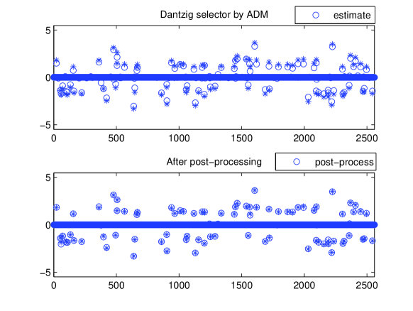
Figure 1: Recovery result for unit-column-normed $X$ from ADM, $\sigma=0.05$

.

Figure 2: Recovery result for unit-column-normed $X$ from AT2, $\sigma=0.05$

.

3.2 Design matrix with orthogonal rows

In this subsection, we consider design matrices with orthogonal rows. We first generate an $n\times p$ matrix $Y$ with independent Gaussian entries and then set $X$ to be the matrix whose rows form an orthogonal basis of the row space of $Y$. The vector $y$ is then generated similarly as in the previous subsection. In particular, we choose $\sigma=0.01$, $0.05$, which corresponds to $1\%$ and $5\%$ noise, $(n,p,s)=(720i,2560i,80i)$ for $i=1,...,10$, and $\delta=\sqrt{2\log(p)}\,\sigma$. For each $(n,p,s)$, we randomly generate $10$ copies of instances. We set $\mu=1/\delta$ and $tol=2e-4$ for the ADM.

The computational results averaged over 10 instances are reported in Tables 3 and 4. For $\sigma=0.01$, we observe from Table 3 that our method generally outperforms the first-order methods implemented in the TFOCS package [3] in terms of both CPU time and solution quality. In particular, comparing with AT2, which produces solutions with the best quality among the first-order methods, our method is at least three times faster and produces solutions with smaller pre-processing errors and comparable post-processing errors. On the other hand, for $\sigma=0.05$, we see from Table 4 that our ADM usually outperforms the first-order methods in terms of solution quality. In addition, our method is faster than AT2 which produces solutions with the best quality among the first-order methods.

In Figure 3, we present the result for one instance with size $(n,p,s)=(720,2560,80)$ and $\sigma=0.05$. The asterisks are the true values of $\beta$ while the circles are the estimates obtained by our method before the post-processing (the upper plot) and after the post-processing (the lower plot). We see from the plot that the latter estimates are very close to the true values of $\beta$. The similar phenomenon can also be observed in Figure 4 for the estimates obtained by AT2 on the same instance.

Table 3: Results for orthogonal $X$, $\sigma=0.01$

			iter			cpu			$\rho^{2}$($\rho^{2}_{\rm orig}$)
$n$	$p$	$s$	ADM	AT1	AT2	ADM	AT1	AT2	ADM	AT1	AT2
720	2560	80	32	394	602	1.3	4.8	7.2	5.0(84.2)	5.6(105.0)	5.1(90.8)
1440	5120	160	28	362	602	7.5	19.4	32.3	4.3(100.1)	5.2(140.7)	4.5(111.5)
2160	7680	240	25	388	602	15.0	43.8	68.0	5.0(102.0)	5.8(141.2)	4.9(110.5)
2880	10240	320	26	398	601	26.8	76.6	116.1	5.1(113.7)	5.8(158.5)	5.1(124.8)
3600	12800	400	25	389	602	38.3	115.0	177.8	4.9(110.0)	5.5(153.2)	4.8(119.9)
4320	15360	480	26	388	601	55.7	162.8	251.7	5.0(110.5)	5.6(151.9)	4.8(118.8)
5040	17920	560	25	389	602	72.2	221.0	341.6	4.6(112.9)	5.3(158.3)	4.6(122.0)
5760	20480	640	25	384	602	93.3	283.1	443.4	4.9(114.5)	5.5(158.3)	4.9(125.8)
6480	23040	720	23	394	601	111.5	365.7	557.3	4.9(117.5)	5.5(159.5)	4.8(126.5)
7200	25600	800	24	392	602	139.9	446.9	686.6	4.8(116.8)	5.5(162.3)	4.8(123.6)

Table 4: Results for orthogonal $X$, $\sigma=0.05$

size			iter			cpu			$\rho^{2}$($\rho^{2}_{\rm orig}$)
$n$	$p$	$s$	ADM	AT1	AT2	ADM	AT1	AT2	ADM	AT1	AT2
720	2560	80	165	227	440	3.3	2.7	5.1	4.9(88.9)	5.7(103.2)	4.9(92.0)
1440	5120	160	149	225	408	20.5	12.3	22.2	5.1(97.4)	5.9(114.1)	5.5(101.3)
2160	7680	240	137	217	408	40.3	24.8	46.5	5.1(98.4)	5.5(112.3)	5.1(101.1)
2880	10240	320	129	220	405	65.7	42.7	78.0	4.9(108.4)	5.5(125.1)	5.0(112.1)
3600	12800	400	145	219	406	110.3	65.1	120.2	5.4(108.3)	6.2(126.4)	5.7(111.5)
4320	15360	480	132	218	405	140.6	92.2	170.9	5.1(107.4)	5.6(121.4)	5.3(110.7)
5040	17920	560	125	211	409	182.3	121.3	233.1	4.9(108.6)	5.4(124.6)	5.1(110.7)
5760	20480	640	115	219	404	219.5	162.4	298.7	4.9(110.4)	5.3(126.8)	5.0(113.8)
6480	23040	720	133	222	404	310.0	207.9	376.9	5.4(117.3)	6.2(134.5)	5.5(121.1)
7200	25600	800	119	217	405	345.9	249.8	464.9	5.0(114.8)	5.6(130.1)	5.1(118.0)

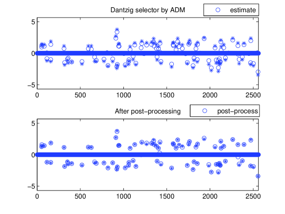
Figure 3: Recovery result for orthogonal $X$, $\sigma=0.05$

.

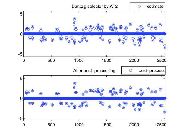
Figure 4: Recovery result for orthogonal $X$, $\sigma=0.05$

.

References

- [1] M. Afonso, J. Bioucas-Dias and M. Figueiredo. An augmented Lagrangian approach to the constrained optimization formulation of imaging inverse problems. Submitted to The IEEE Transactions on Image Processing (2009).
- [2] A. Auslender and M. Teboulle. Interior gradient and proximal methods for convex and conic optimization. SIAM Journal on Optimization 16, pp. 697–725 (2006).
- [3] S. Becker, E. Candès and M. Grant. Templates for convex cone problems with applications to sparse signal recovery. Preprint at arXiv:1009.2065v2 [math.OC].
- [4] D. Bertsekas and J. N. Tsitsiklis. Parallel and Distributed Computation: Numerical Methods. Prentice Hall (1989).
- [5] P. J. Bickel. Discussion: the Dantzig selector: statistical estimation when is much larger than . Annals of Statistics 35, pp. 2352–2357 (2007).
- [6] T. T. Cai and J. Lv. Discussion: the Dantzig selector: statistical estimation when is much larger than . Annals of Statistics 35, pp. 2365–2369 (2007).
-
[7]
E. Candès and J. Romberg.
-magic : recovery of sparse signals via convex programming.
User guide, Applied & Computational Mathematics, California Institute of Technology,
Pasadena, CA 91125, USA, October 2005.
Available at
www.l1-magic.org. - [8] E. Candès and T. Tao. The Dantzig selector: statistical estimation when is much larger than . Annals of Statistics 35, pp. 2313–2351 (2007).
- [9] E. Candès and T. Tao. Rejoinder: the Dantzig selector: statistical estimation when is much larger than . Annals of Statistics 35, pp. 2392–2404 (2007).
- [10] J. Eckstein and D. Bertsekas. On the Douglas-Rachford splitting method and the proximal point algorithm for maximal monotone operators. Mathematical Programming 55, pp. 293–318 (1992).
- [11] B. Efron, T. Hastie and R. Tibshirani. Discussion: the Dantzig selector: statistical estimation when is much larger than . Annals of Statistics 35, pp. 2358–2364 (2007).
- [12] E. Esser, X. Zhang and T. Chan. A general framework for a class of first order primal-dual algorithms for TV minimization. UCLA CAM Report 09-67 (2009).
- [13] M. P. Friedlander and M. A. Saunders. Discussion: the Dantzig selector: statistical estimation when is much larger than . Annals of Statistics 35, pp. 2385–2391 (2007).
- [14] G. M. James, P. Radchenko and J. Lv. DASSO: connections between the Dantzig selector and lasso. Journal of the Royal Statistical Society B 71, pp. 127–142 (2009).
- [15] G. Lan, Z. Lu and R. D. C. Monteiro. Primal-dual first order methods with iteration-complexity for cone programming. To appear in Mathematical Programming, DOI: 10.1007/s10107-008-0261-6.
- [16] Z. Lu. Primal-dual first-order methods for a class of cone programming. Technical report, Department of Mathematics, Simon Fraser University, Burnaby, BC, V5A 1S6, Canada, September 2009.
- [17] Z. Lu and Y. Zhang. An augmented Lagrangian approach for sparse principal component analysis. Technical report, Department of Mathematics, Simon Fraser University, Burnaby, BC, V5A 1S6, Canada, July 2009.
- [18] N. Meinshausen, G. Rocha and B. Yu. Discussion: a tale of three cousins: lasso, L2boosting and Dantzig. Annals of Statistics 35, pp. 2373–2384 (2007).
- [19] Y. Nesterov. A method for solving a convex programming problem with convergence rate . Soviet Mathematics Doklady 27, pp. 372–376 (1983).
- [20] Y. Nesterov. Gradient methods for minimizing composite objective function. Technical Report 2007/76, CORE, Université catholique de Louvain (2007).
- [21] Y. Ritov. Discussion: the Dantzig selector: statistical estimation when is much larger than . Annals of Statistics 35, pp. 2370–2372 (2007).
- [22] J. K. Romberg. The Dantzig selector and generalized thresholding. In Proceedings of IEEE Conference on Information Science and Systems, Princeton, New Jersey, February 2008.
- [23] R. Tibshirani. Regression shrinkage and selection via the lasso. Journal of Royal Statistical Society B 58, pp. 267–288 (1996).
- [24] P. Tseng. On accelerated proximal gradient methods for convex-concave optimization. Submitted to SIAM Journal on Optimization (2008).
- [25] J. Yang and Y. Zhang. Alternating direction algorithms for -problems in compressive sensing. TR09-37, CAAM, Rice University (2009).
- [26] J. Yang, Y. Zhang and W. Yin. A fast alternating direction method for TVL1-L2 signal reconstruction from partial Fourier data. IEEE Journal of Selected Topics in Signal Processing 4, pp. 288–297 (2010).
- [27] X. Yuan. Alternating direction methods for sparse covariance selection. Preprint (2009).
- [28] H. Zou and T. Hastie. Regularization and variable selection via the elastic net. Journal of Royal Statistical Society B 67, pp. 301–320 (2005).