The PRIsm MUlti-Object Survey (PRIMUS) I: Survey Overview and Characteristics
Abstract
We present the PRIsm MUlti-object Survey (PRIMUS), a spectroscopic faint galaxy redshift survey to . PRIMUS uses a low-dispersion prism and slitmasks to observe 2,500 objects at once in a 0.18 deg2 field of view, using the IMACS camera on the Magellan I Baade 6.5m telescope at Las Campanas Observatory. PRIMUS covers a total of 9.1 deg2 of sky to a depth of in seven different deep, multi-wavelength fields that have coverage from GALEX, Spitzer and either XMM or Chandra, as well as multiple-band optical and near-IR coverage. PRIMUS includes 130,000 robust redshifts of unique objects with a redshift precision of . The redshift distribution peaks at and extends to for galaxies and for broad-line AGN. The motivation, observational techniques, fields, target selection, slitmask design, and observations are presented here, with a brief summary of the redshift precision; a companion paper presents the data reduction, redshift fitting, redshift confidence, and survey completeness. PRIMUS is the largest faint galaxy survey undertaken to date. The high targeting fraction (%) and large survey size will allow for precise measures of galaxy properties and large-scale structure to .
Subject headings:
Surveys – galaxies: distances and redshifts – galaxies: evolution – galaxies: high-redshift – cosmology: large-scale structure of universe1. Introduction
Redshift surveys are a crucial tool for understanding galaxy evolution. As pioneering large redshift surveys of the local Universe dramatically demonstrated (e.g., the CfA survey, Davis et al. 1982), redshifts remove the effects of projection, reveal the cosmic web, and allow conversion of observed fluxes and sizes to physical restframe quantities. Armed with redshifts, one can determine key statistical properties of galaxy populations such as luminosity functions, merger rates, and correlation functions, across cosmic time. Combining redshifts with multi-wavelength imaging from the ultraviolet (UV) to the infrared (IR) allows one to further measure star formation rates (SFRs) and stellar masses, while X-ray data allow studies of AGN properties.
At low redshift, the largest galaxy redshift surveys are the Sloan Digital Sky Survey (SDSS, York et al. 2000), the Two Degree Field Galaxy Redshift Survey (2dFGRS, Colless et al. 2001), and the Six Degree Field Galaxy Redshift Survey (6dFGS, Jones et al. 2009). These surveys extend to and contain hundreds of thousands of galaxy redshifts, mapping out volumes of Mpc-3 and Mpc-3 for 2dFGRS and SDSS, respectively. Enormous datasets of this size are required to both overcome the cosmic variance of large-scale clustering and to measure joint distributions of properties such as color and luminosity across a range of environments. It is only through studying joint properties of galaxies as well as their full distribution functions, spanning a wide range of redshifts, that the evolution of galaxies will be understood.
Several flux-limited redshift surveys have begun to probe initial volumes of the distant universe. At intermediate redshift, the AGN and Galaxy Evolution Survey (AGES, Kochanek et al. in preparation) is a wide-field survey that has obtained redshifts for 13,000 galaxies over 8 deg2 to . The median redshift of the AGES galaxy sample is . Deeper surveys have targeted the more distant universe; the largest of these include COMBO-17 (Wolf et al. 2003), DEEP2 (Davis et al. 2003, Faber in preparation), the VIMOS VLT Deep Survey (VVDS, Le Fèvre et al. 2005; Garilli et al. 2008), and zCOSMOS (Lilly et al. 2007). Of these, the largest area surveyed is the VVDS-Wide survey, which has covered 6 deg2 to a depth of ; the other surveys cover half this area, at most. The deepest of these surveys are DEEP2, which covered 3 deg2 to a depth of , and VVDS-Deep, which covered 0.6 deg2 to a depth of . The largest samples in terms of number of redshifts are the DEEP2 and VVDS-Wide surveys, with 30,000 and 20,000 current secure redshifts each. The median redshift of these samples is . Surveys at higher redshift () have not been flux-limited in a single photometric band, but rather use various color-selection techniques to identify galaxy candidates at specific redshifts (e.g., Steidel et al. 2004; Quadri et al. 2007; van Dokkum et al. 2009), resulting in samples of typically a few thousand objects.
What is currently known about galaxy evolution results from surveys that extend to high redshift; however, the sample sizes and volumes mapped by these surveys are still relatively small compared to low redshift samples. The samples are not large enough to measure, for example, the luminosity function of blue and red galaxies in multiple bins in redshift and environment. The dominant error in most statistical studies at is cosmic variance111E.g., in the COSMOS field, 1.4 deg. on a side, the fractional error in a count of an unbiased tracer of mass is 9% at in a bin.; the volumes that have been surveyed are not yet large enough to fully sample the overdensity distribution at a given redshift. An additional complication in trying to measure the evolution of a given galaxy statistic is that there is often a gap in redshift between low redshift samples at and higher redshift samples at . The deeper surveys do not have sufficiently large numbers of sources or survey sufficient volumes at intermediate redshifts of to continuously track a statistic over cosmic time with small error bars. While the AGES survey addresses this gap to some degree, it is not sufficiently deep to overlap the higher redshift surveys substantially in redshift. What is needed are significantly larger surveys at intermediate redshift that are 1) large enough to have comparable errors to local surveys such as 2dFGRS and SDSS, 2) deep enough to sample typical galaxies at intermediate redshift, and 3) have the requisite multi-wavelength imaging needed to measure SFRs and stellar masses.
The deep, multi-wavelength imaging extending beyond the optical regime that is required to carry out such a survey at intermediate redshifts is now available. Simultaneous with the spectroscopic advances that have allowed the first redshift surveys to to be carried out, astronomy has entered a golden age in wide-field imaging, both to survey local galaxies and those at . Modern imaging surveys have mapped a large volume () at redshift in the ultraviolet with the Galaxy Evolution Explorer (GALEX, Martin et al. 2005), in the optical with SDSS, and in the near-IR with the 2-Micron All Sky Survey (2MASS, Skrutskie et al. 1997). The similarly ambitious United Kingdom Infrared Deep Sky Survey (UKIDDS, Lawrence et al. 2007) near-IR survey is conducting a survey of 7500 deg2 to , and the Wide-field Infrared Survey Explorer (WISE, Liu et al. 2008), which will survey the entire sky in the mid-IR (m), launched in late 2009. Even more remarkable is that a similar volume has recently become available at . The UKIDDS deep survey to , the Spitzer Wide-area Infrared Extragalactic Survey (SWIRE, Lonsdale et al. 2003), the Spitzer Deep, Wide-Field Survey (SDWFS Ashby et al. 2009) and Spitzer GTO shallow program (Eisenhardt et al. 2004), the GALEX Deep Imaging Survey (DIS), and companion deep optical imaging are covering about 70 deg2 to depths that reach below at from the UV to the far-IR.
These deep imaging surveys can be harnessed to study galaxy evolution using volumes sufficient to overcome cosmic variance, but only by coupling them to large redshift surveys. Only with redshifts can restframe properties such as luminosities, colors, SFRs, and stellar masses be robustly measured. The goal of the PRIsm MUlti-object Survey (PRIMUS), which we present here, is to provide the spectroscopy necessary to make this science possible. PRIMUS is the largest faint galaxy redshift survey performed to date. PRIMUS has targeted multiple fields with existing deep optical imaging, UV GALEX imaging, IR Spitzer/IRAC and MIPS imaging, and X-ray Chandra and/or XMM coverage in order to provide the data to address these issues. By obtaining low-resolution spectra with a slitmask and prism, we have assembled a unique and unprecedentedly large data set containing 120,000 redshifts to (and 9,000 stars), covering over 9.1 deg2 of sky with complementary multi-wavelength imaging. Using the IMACS instrument on the Magellan telescope, which has a wide 0.2 deg2 field, with a prism we observed 2,500 targets simultaneously to depths of in one hour. We observed 10,000 target galaxies per night, substantially larger than traditional spectroscopic surveys undertaken at Keck and VLT. Our survey has a redshift precision of %, which is the precision required to measure galaxy environments and clustering statistics. This survey is approximately four times larger than DEEP2 and covers one half the volume of 2dFGRS, but at a mean redshift of (for the joint sample of galaxies and broad-line AGN).
This paper describes the design, survey characteristics, and data taken for PRIMUS, which is a collaboration between astronomers at the University of Arizona, the University of California at San Diego, New York University, and Princeton University. A companion paper (Cool et al. in preparation) describes the data reduction, redshift fitting algorithm, redshift assessment and completeness, as well as lessons learned from carrying out the survey. The outline of this paper is as follows. Section 2 describes the motivation for and goals of our survey. Section 3 summarizes the hardware built for and used by the survey, namely the prism and IMACS camera. Section 4 provides information about the fields observed by the survey, while Section 5 outlines the algorithms used to select targets for slitmasks and Section 6 presents the mask design considerations. Section 7 describes how the observations were carried out, and Section 8 provides detailed information on the various optical photometric datasets used in each field, including derived zeropoints. A summary of the observed PRIMUS data and a comparison to other surveys is provided in Section 9. Throughout the paper, AB magnitudes are used.
2. The Motivation for Low Resolution Spectroscopy
High-precision spectroscopic redshifts are the gold standard for determining distances to galaxies outside the local Universe. However, conventional spectroscopy of large numbers of faint galaxies is observationally extremely expensive, particularly over the wide areas needed to suppress the effects of cosmic variance — the fact that large-scale structure can greatly affect the density in any particular, small patch of the Universe we map. Existing deep, wide-field, multi-wavelength imaging exceeds its spectroscopic reach by at least a factor of 10, and conducting a survey of hundreds of thousands of galaxies to would require a mammoth and unfeasible investment of time for a high resolution spectroscopic survey on the current, existing instruments. Low-precision broad-band photometric redshifts are commonly used to fill this gap and have become popular because they are much easier to acquire and therefore can be done for much larger data sets (e.g., Budavari et al. 2003; Mobasher et al. 2004; Padmanabhan et al. 2005; Gladders & Yee 2005; Pelló et al. 2009; Adami et al. 2010). However, the usual broad-band (–) photometric redshifts are susceptible to systematic errors, have a non-trivial fraction of catastrophic failures (10%), and typically have 5% redshift errors, which are large compared to the physical clustering lengths. Several recent efforts involve combining both optical and NIR imaging, though the redshift error is still 4-5% (Brodwin et al. 2006; Rowan-Robinson et al. 2008). The best photometric redshifts published that use several broad-band filters are those from CFHTLS, which have 3-4% redshift errors and 2-4% catastrophic outliers (defined as ), depending on the depth of the sample (Coupon et al. 2009); these rates are better than other surveys due to the depth of the imaging data.
Systematic errors on the redshifts are often the limiting uncertainty in the quantification of galaxy properties and clustering from surveys that rely on this technique. Errors of a few percent in distance produce significant uncertainties in flux-dependent quantities such as stellar mass and SFR, and they create punishing background subtraction problems for clustering and environment analyses of any sort. Errors of 0.5% alleviate all of these problems, especially when studying clustering statistics. For example, at an error of 5% in leads to an error of 0.4 magnitudes in the distance modulus, while an error of 0.5% in leads to an error of 0.04 magnitudes.
The COMBO-17 survey (Wolf et al. 2003, 2004) achieved considerable success with a hybrid technique, in which twelve intermediate-band optical images plus five broad-band images were used to create a 10-15 spectrum. Having somewhat higher resolution allows COMBO-17 to identify the spectral energy distribution (SED) breaks more accurately, thereby improving their redshift precision to 3% and reducing the number of outliers. The COSMOS team has since followed suit and obtained 30 bands of photometry over 2 deg2 to obtain 0.7% redshifts to at a depth of (Ilbert et al. 2009). For reference, the imaging for 20 of these photometric bands was obtained at the Subaru 8m telescope and required 20 nights of observing.
However, these surveys with more than ten bands of photometry cover only 1–2 deg2 of sky, as the exposure time of a intermedian-band imaging survey scales roughly as : one factor of for the number of filters, the other for the length of each exposure to reach a given signal-to-noise (S/N) ratio. This scaling means that even wide-field photometric surveys are highly inefficient, and the current best photometric redshift surveys over wide areas have a precision of 3-4% (CFHTLS, Coupon et al. 2009). The major source of inefficiency is that nearly all of the pixels to are blank sky. It is much more efficient to disperse the light and use more of the detector pixels on sources. With dispersion, exposure times scale only as one power of to reach a given S/N per resolution element. For , this factor is more than sufficient to pay off the throughput penalties of the spectrograph or the need to use two masks to mitigate slit collisions.
With PRIMUS, we have used the IMACS instrument on the 6.5m Magellan telescope to obtain both a significantly higher survey speed and spectroscopic resolution () than even the best photometric redshift surveys, e.g., COMBO-17 and the COSMOS 30-band photometric redshifts. By using the detector pixels to multiplex spectrally instead of integrating on blank sky, we cut the survey time by a substantial factor while gaining higher spectral resolution.
In general, the advantage of low-resolution spectroscopy compared to intermediate-band photometric redshifts depends on the relative fields of view, throughputs, and apertures of the facilities as well as on the target density and completeness requirements for the science goals. Higher target densities favor imaging surveys, because there is less blank sky; lower target densities favor spectroscopic surveys, as one can fill more of the sky with higher spectral resolution data. Some science cases depend sensitively on high survey completeness; others require only statistical control of the incompleteness. Additional less important factors are that, compared to spectroscopy, photometry allows one to optimally weight the radial profile of the target and to avoid losing light at a slit. Conversely, spectroscopy allows one to obtain continuous spectral sampling, as opposed to fixed filters, and to optimally weight the spectral information, e.g., to downweight information at the wavelength of sky lines.
As we show in Section 9 and in Cool et al. (in preparation), our spectra result in redshifts precise to . They also provide medium-band SEDs and detection of the strongest emission lines and broad AGN lines. Given the relatively low dispersion of our spectra, we do not attempt to measure detailed line diagnostics for individual sources nor the internal velocity distributions of groups and clusters, given our redshift precision. However, redshift-space distortions smear out the cosmic web by , such that redshifts more accurate than about 1% do not improve most clustering or environment analyses, which integrate over these distances anyway. For our science goals, therefore, exchanging higher resolution redshifts for a faster, wider redshift machine is a very worthwhile trade, and is the only currently feasible way to obtain redshifts of large samples over wide areas of sky. Future very wide-field spectroscopic instruments may provide an alternative route, though these spectrographs do not currently exist. We emphasize that any existing wide-field multi-object spectrograph would benefit from multiplexing using a low-dispersion prism. For PRIMUS, IMACS on Magellan is ideally suited given the relatively large field of view of 0.18 deg2.
We use the near-IR, mid-IR, UV, and X-ray data in our fields as proxies for stellar mass, star formation, and AGN activity. Optical emission and absorption lines provide alternative approaches to these measurements, but require spectra of far better quality than what is needed to measure a redshift. Given the existence of the multi-wavelength imaging in our fields, our goal is to efficiently obtain spectra over a wide area in order to determine redshift measurements.
3. Prism and Camera Characteristics
| \colrule\colrule | ||||||||||||
|---|---|---|---|---|---|---|---|---|---|---|---|---|
| Field name | RAaaaApproximate center of field observed by PRIMUS | Dec | AreabbbArea over which PRIMUS obtained spectroscopy; regions not surveyed due to bright stars, missing photometry, and CCD chip gaps have been removed | cccNumber of slitmasks observed | dddNumber of primary and total targets observed, duplicate observations are not included (see text for details) | eeeNumber of stars, galaxies+AGN, and primary objects (stars+galaxies+AGN) with robust redshifts, defined as Q=3 or 4 (see Section 9) | SpitzerfffArea with joint PRIMUS and either Spitzer, GALEX, Chandra or XMM coverage. | GALEX | X-ray | |||
| (J2000) | (J2000) | (deg2) | observed | robust z | (deg2) | |||||||
| \colrule\colrule | ||||||||||||
| CDFS-SWIRE | 03:32 | -28:54 | 1.95 | 29 | 46,127 | 33,970 | 933 | 22,898 | 19,942 | 1.94 | 1.95 | |
| COSMOS | 10:00 | +02:21 | 1.03 | 18 | 39,971 | 20,741 | 2,162 | 17,963 | 11,230 | 1.03 | 1.03 | 1.03 |
| DEEP2 02hr | 02:30 | +00:36 | 0.58 | 8 | 14,213 | 9,814 | 99 | 7,289 | 5,778 | 0.47 | 0.31 | 0.52 |
| DEEP2 23hr | 23:30 | +00:09 | 0.67 | 10 | 15,604 | 10,491 | 87 | 7,329 | 5,811 | 0.67 | 0.67 | |
| DLS F5 | 13:58 | -11:18 | 1.04 | 13 | 30,653 | 22,895 | 1,218 | 11,032 | 10,147 | |||
| ELAIS S1 | 00:36 | -43:30 | 0.90 | 12 | 21,534 | 15,839 | 842 | 9,992 | 9,101 | 0.90 | 0.86 | 0.52 |
| XMM-LSS | 02:20 | -04:45 | 2.88 | 42 | 102,218 | 61,689 | 3,364 | 44,451 | 34,590 | 2.84 | 2.65 | 2.77 |
| \colrule | ||||||||||||
| Total | 9.05 | 132 | 270,320 | 175,439 | 8,705 | 120,954 | 96,599 | 7.18 | 7.47 | 5.51 | ||
PRIMUS was conducted with the Inamori Magellan Areal Camera and Spectrograph (IMACS, Bigelow & Dressler 2003) operating on the Magellan I (Baade) Telescope at Las Campanas Observatory. The IMACS f/2 camera delivers a square field of view with slight vignetting, for an active area of 0.18 deg2. The pixel scale is per pixel, so our spectra are well-sampled. The detector has eight 2k4k15 micron CCDs. The chip gaps are 11.4 between the short sides of the CCDs and 18.4 between the long sides. Using the fast readout mode, the gain is e-/adu and the read noise is 4 e-/pixel.
As with traditional spectroscopy programs, PRIMUS used custom-designed slitmasks, made with the laser mask miller at Las Campanas. The bulk of the survey used a slit size of wide by long. Details of the mask design are given in Section 6. The innovative design aspect of PRIMUS is to use a prism in the place of the transmission gratings normally used with the f/2 camera. The prism was designed and fabricated for our survey; it was mounted in IMACS in January 2006 and was immediately made available to general users. The prism is made of three pieces of glass, one piece of PBM2Y glass in between two pieces of FSL5Y glass (all i-line glasses from O’Hara). The size is 190 mm in diameter by 84mm depth at its thickest point. The total cost of the prism and mounting was K.
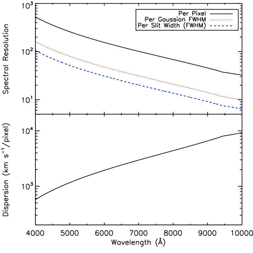
As a dispersing element, a prism is ideal in that it has a very broad transmission curve, extremely high throughput, requires no order blocking filters, and does not exhibit excessive scattered light compared to transmission gratings. Additionally, because of the wide field of view of the f/2 camera, grisms operating at 100 lines mm-1 and below will be strongly affected by zero-order direct images of the slits. A prism does not suffer from this effect. It also has no blaze condition and has a higher throughput over a wider wavelength range compared to gratings and grisms. The low-dispersion prism designed for PRIMUS yields spectra from 3900Å to 1 m that requires only 150 pixels in the spectral direction, a tiny fraction (2%) of the IMACS f/2 field of view. We are therefore able to multiplex both spatially and spectrally to observe galaxies at once. Figure 1 shows the wavelength-dependent spectral resolution (top panel) and dispersion (bottom panel) of the prism, which changes considerably from blue to red. The throughput of the prism is %, and the overall throughput of the prism plus camera, including the telescope but not the atmosphere, peaks at 24% at 6900 Å, is 20% at 5200 and 7600 Å, and is 10% at 4450 and 8500 Å.
4. Fields
PRIMUS primarily targeted regions of the sky with existing deep multi-wavelength imaging. Our goal was to cover all of the southern SWIRE fields that had pre-existing optical photometry from which we could design slitmasks. In order to facilitate being able to observe for full nights over roughly half of the year, we also observed several non-SWIRE fields, some of which have deep Spitzer data. All but one of our fields have GALEX coverage and all but two have X-ray coverage from either Chandra or XMM. These fields are designated as “science fields.” We also targeted a small number of “calibration fields” that have existing high-resolution spectroscopic redshifts from other surveys, which we use to characterize our redshift accuracy and precision.
PRIMUS observed a total of ten independent fields, seven science and three calibration fields. The science fields include the Chandra Deep Field South-SWIRE field (CDFS-SWIRE, which is not centered on the CDFS proper, Giacconi et al. 2001), the 23hr and 02hr DEEP2 fields, the COSMOS field, the European Large Area ISO Survey - South 1 field (ELAIS-S1, Oliver et al. 2000), the XMM-Large Scale Structure Survey field (XMM-LSS, Pierre et al. 2004), and the Deep Lens Survey (DLS, Wittman et al. 2002) F5 field. Of these, SWIRE coverage exists for the CDFS, ELAIS-S1, and XMM-LSS fields, and S-COSMOS (Sanders et al. 2007) provides deep Spitzer coverage of the COSMOS field. X-ray coverage exists for both DEEP2 fields (Chandra), the XMM-LSS field (XMM), and the COSMOS and ELAIS-S1 fields (both Chandra and XMM). The total area with joint PRIMUS and either Spitzer, GALEX or X-ray coverage is 7.18 deg2, 7.47 deg2, and 5.51 deg2, respectively.
Details of the PRIMUS science fields are given in Table 1. Listed are the approximate field centers as observed by PRIMUS, the total area targeted, the number of slitmasks observed, and the number of unique targets and robust redshifts derived in each field, along with the area of each field that contains multi-wavelength coverage. We separately list the number of stars versus galaxies and AGN that have robust redshifts. Robust redshifts are defined as having a redshift confidence flag Q3 or 4; see Section 9 for details. The numbers listed for the primary sample include stars, galaxies, and AGN. The areas listed in Table 1 are the total area that has PRIMUS targets and are conservative in that they do not include regions masked by bright stars, missing photometry, or that fell in between chip gaps on the CCD. If these areas are included then the total area of the survey is 10.78 deg2.
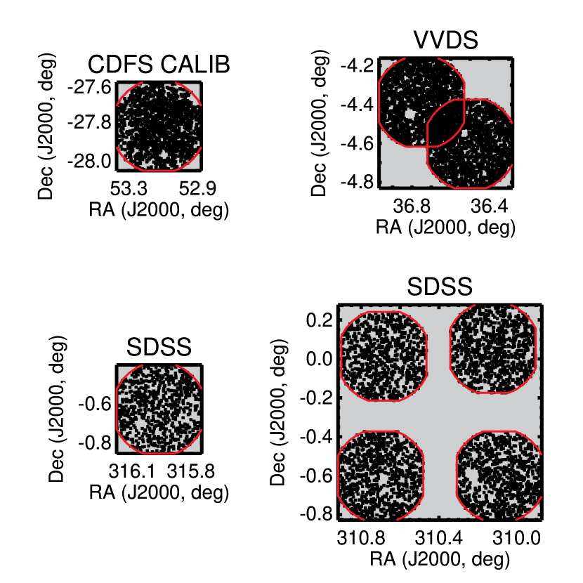
Table 2 provides information on the PRIMUS coverage of the calibration fields, which include the original CDFS (which has high-resolution spectroscopic redshifts from the VVDS), the deep VVDS field, and a portion of the SDSS equatorial Stripe 82 (Abazajian et al. 2009). The DEEP2 02hr and 23hr fields and the COSMOS field are used as both science and calibration fields.
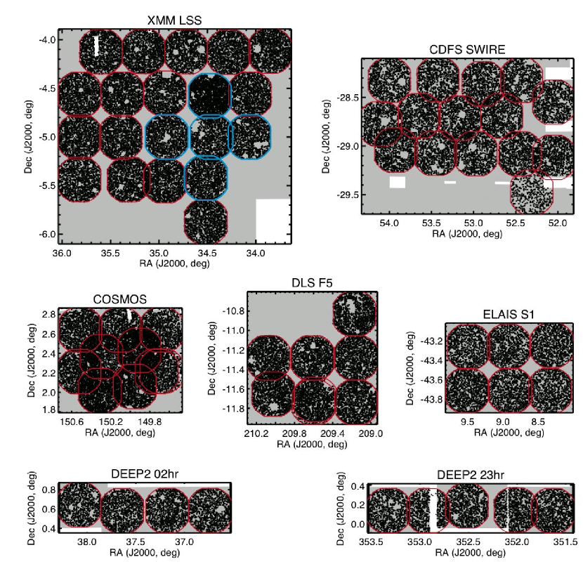
Figures 2 and 3 show the PRIMUS sky coverage in our science and calibration fields. The light grey areas indicate photometric coverage of the catalog used for targeting, red lines outline the observed PRIMUS slitmasks, and the black crosses show PRIMUS targets, where we plot a random 20% of the total targets for clarity in the science fields and 50% of the targets in the calibration fields. In the XMM-LSS field, five PRIMUS pointings are outlined in cyan; in this area we used photometry from the Subaru/XMM-Newton Deep Survey (SXDS, Furusawa et al. 2008) for targeting (see the next section for details). During targeting, areas around bright stars were masked to avoid photometric errors. These regions can be seen as grey areas within the PRIMUS masks that do not have targets.
| \colrule\colrule | |||||||||
|---|---|---|---|---|---|---|---|---|---|
| Field name | RAaaaColumn meanings are identical to Table 1 | Dec | Area | ||||||
| (J2000) | (J2000) | (deg2) | observed | robust z | |||||
| \colrule\colrule | |||||||||
| CDFS-CALIB | 03:32 | -27:49 | 0.15 | 3 | 1,841 | 0 | 82 | 1,197 | 0 |
| SDSS | 20:52 | -00:18 | 0.74 | 5 | 7,571 | 6,100 | 1,773 | 2,572 | 3,534 |
| VVDS | 02:26 | -04:36 | 0.27 | 2 | 5,876 | 0 | 132 | 2,672 | 0 |
| \colrule | |||||||||
| Total | 1.16 | 10 | 15,288 | 6,100 | 1,987 | 6,441 | 3,534 | ||
| \colrule | |||||
| Field name | Telescope | 100% samplingaaaPhotometric band and depth of primary sample used for spectroscopic target selection. See §5.1.1 for details. | 30% sampling | Non-primary limiting | referencebbbReference for photometric catalog |
| mag (AB) | mag range (AB) | mag (AB) | |||
| \colrule\colrule | |||||
| CDFS-SWIREcccThese fields have an additional IRAC 3.6 m flux limit of 10 mJy. See §5.1 for details. | CTIO/Blanco | Lonsdale et al. (2003) | |||
| COSMOS | HST/ACS | dddF814W band | Koekemoer et al. (2007) | ||
| DEEP2 02hr | CFHT | Coil et al. (2004) | |||
| DEEP2 23hr | CFHT | Coil et al. (2004) | |||
| DLS F5 | CTIO/Blanco | Wittman et al. (2006) | |||
| ELAIS S1cccThese fields have an additional IRAC 3.6 m flux limit of 10 mJy. See §5.1 for details. | ESO/WFI | Berta et al. (2006) | |||
| XMM-LSS/CFHTLS | CFHT | T0003 release eeehttp://terapix.iap.fr | |||
| XMM-LSS/SXDS | Subaru | Furusawa et al. (2008) | |||
| \colrule |
5. Target Selection
5.1. Overview of Target Selection
The goal of PRIMUS was to obtain redshifts for a flux-limited, high-density sample of galaxies, spanning all galaxy types, over a wide area to . Pushing to would require higher-resolution spectroscopy than was available with the low-dispersion prism that we used. Additionally, one needs to sample redward of the 4000 Å break reasonably well, and the spectral resolution is particularly low at the red end of our spectra (see Figure 1).
We used existing photometry in each field to choose targets for spectroscopy. The imaging data used in each field for targeting is at least one magnitude deeper than our targeting limit. As the imaging was taken from several different sources (using different cameras on different telescopes), it is not expected to be perfectly homogeneous. The differences in targeting photometric band and depth can and will be accounted for when correcting for the survey completeness and will be performed for all relevant science papers.
In order to maximize the area of the survey, thereby minimizing cosmic variance errors, we limited our total exposure time per slitmask to 1 hour. In the COSMOS field we exposed for 1.5 hours to reach a higher S/N in our spectra and to target to a slightly fainter depth, due to the high-quality, deep ancillary multi-wavelength data and HST imaging in that field.
We generally targeted all galaxies to and sparse-sampled objects with well-defined a priori sampling rates. In this way PRIMUS would not be dominated by galaxies at our faintest flux limits. Because the targeting and selection weights were all tracked and saved, a statistical complete sample to can be created from the PRIMUS data. As the low-dispersion spectroscopy technique we used was experimental, we intentionally targetted fainter galaxies, with the intention of determining the redshift success thresholds from the spectroscopic data. The result is that our success rate is a function of magnitude (as discussed below and in detail in Cool et al. in preparation, and we failed on a fair fraction of the fainter targets below .
Three fields have SWIRE coverage: CDSF-SWIRE, ELAIS-S1, and XMM-LSS. In the CDFS-SWIRE and ELAIS-S1 fields (but not the XMM-LSS field), due to a bug in the design code, at only objects with IRAC counterparts brighter than 10 mJy at 3.6 m in the SWIRE catalog were targeted. This leads to an additional selection effect that will be accounted for in relevant science papers. In all three of the SWIRE fields, we intentionally additionally targeted sources to that were bright at 3.6 m (10 mJy in a 3.8 aperture), and sources to that were detected in the IRAC 5.8, 8.0, or MIPS 24 m bands. In the XMM-LSS field, we initially designed slitmasks in the SXDS area of the field, which had deep publicly-available Subaru imaging prior to the first CFHTLS imaging release; these masks are outlined in cyan in Figure 2. In the rest of the XMM-LSS field, we used CFHTLS imaging for targeting.
In fields that lacked available or band imaging when we designed our slitmasks, we used band photometry and adjusted the magnitude selection limit such that cumulative galaxy number counts at the magnitude limit were comparable across fields. This procedure corrects for the average color difference of galaxies. We used the star-galaxy separation that was available in the targeting catalogs in each field; the details of this separation are therefore field-dependent.
5.1.1 Primary Sample
Table 3 lists information on the photometry that was used in each field to select targets for spectroscopy and the limiting apparent magnitude of the primary sample. The “primary” sample in each field is defined as those objects from which we can create a statistically complete sample. These objects have a well-understood selection function both in terms of their selection magnitude and their location in the plane of the sky, i.e. they have a recoverable spatial selection. This sample can therefore be used for statistical measurements such as the two-point correlation function and luminosity function, as there is little to no bias in terms of the spatial density in this sample.
5.1.2 Sparse Sampling
From the input photometric catalog used for targeting, we defined two selection weights for each object: (1) a magnitude-dependent sparse-sampling weight, which was used to select a fraction of galaxies at random in the 0.5 magnitude interval above our primary sample targeting limit; and (2) a spatial density-dependent weight, which was used to select galaxies in crowded regions of the sky where the spectra of adjacent galaxies would overlap on the detector. We refer to these two selection weights as the (magnitude-dependent) “sparse-sampling weight” and the (spatially-dependent) “density-dependent weight.” Details of the density-dependent sampling are given in Section 6.2.
The sparse-sampling weight is equal to 1 to the “100% sampling limiting magnitude” in each field (generally ) and equal to either 1 (if spatially isolated) or 0.3 (if there are collisions) in the “30% sampling magnitude range” (generally 0.5 magnitude fainter). In defining these weights, we first checked to see if an object had two nearby neighbors that would have created a collision in designing the slitmasks (see Section 6.2 for details on the definition of nearby neighbors). If an object did not have collisions, then it was not sparse-sampled (i.e. the sparse-sampling weight was 1). If an object had two or more nearby neighbors, it was sparse-sampled with a weight of 0.3.
5.1.3 AGN Selection
When choosing galaxies, we kept point sources if their optical and/or IR colors indicated that they may be AGN. Specifically, point sources that passed any of the following Spitzer color cuts were targeted:
| (1) |
Additional optical color thresholds were used to define AGN candidates in most fields, where the color definitions used depended on the available imaging in each passband. In the CDFS, point sources that passed either of the following optical cuts were targeted:
| (2) | |||
| (3) |
In the COSMOS field, point sources in the HST imaging with were targeted, with no color pre-selection applied. In the two DEEP2 fields, we targeted photometrically-selected AGN with and from Richards et al. (2004). In the SXDS area of the XMM-LSS field, objects that were detected by XMM were selected to . In addition, point sources were targeted if their optical colors indicated that they may be AGN, where the following selection was used:
| (4) |
In the rest of the XMM-LSS field, point sources with that passed either of the following optical cuts were targeted:
| (5) | |||
| (6) |
While the targeting weights of AGN identified by their optical colors vary from field to field, for science purposes we will be able to perform completeness corrections within each field. In general, the X-ray imaging data that exists in these fields will be used to define parent AGN samples. We can then account for our targeting selection effects to define a complete sample of X-ray detected AGN.
In instances where the team that provided the targeting photometry requested spectroscopy of small numbers of specific objects, they were added as high priority filler targets.
5.1.4 Additional Targets
We additionally targeted galaxies at lower priority that did not pass the density-dependent sampling or magnitude-dependent sparse-sampling, often to 0.5 magnitude fainter than the “30% sampling magnitude limit”, if they could be placed on slitmasks without colliding with higher priority, primary targets. Empty slits with no objects were milled in all fields except the DEEP2 02hr and COSMOS fields, to test sky subtraction and extraction. We also observed photometrically-selected F stars as spectrophotometric calibrators on each slitmask, where SDSS imaging was used to select F stars where available. See Cool et al. (in preparation) for information on the data reduction and flux calibration of our spectra.
5.2. Selection Details in Calibration Fields
Target selection in our calibration fields depended on the available high-resolution spectroscopic data. Details of the target selection for each of our calibration fields is given below.
5.2.1 CDFS-CALIB
Three slitmasks were observed in the original CDFS, which has high-resolution spectroscopic redshifts from the VVDS. Priority was given to targets with high-quality VVDS redshifts (rank 3 or higher, Le Fèvre et al. 2005) to . We also targeted galaxies with lower-quality VVDS redshifts (rank 1 or 2), as well as objects with spectroscopic redshifts from the Intermediate Mass Galaxy Evolution Sequence survey (IMAGES, Ravikumar et al. 2007) (rank 1 or 2), and COMBO-17 galaxies with .
5.2.2 DEEP2
The two fall DEEP2 fields are used by PRIMUS for both science and calibration. In these fields, high-resolution spectroscopy is available from the DEEP2 survey for galaxies selected in color-color space to be at to a depth of 111http://deep.berkeley.edu/DR3.
In the region of the 02hr field that has DEEP2 spectroscopy (roughly 75% of the photometric area available), PRIMUS targeted a set of galaxies that is complementary to the DEEP2 sample. PRIMUS targeted galaxies with colors indicating redshifts (i.e. exactly those not targeted by DEEP2) with no sparse-sampling to and 100% of the non-collided and 30% of the collided galaxies with . Slitmasks were then filled with galaxies that had DEEP2 redshifts to , to use in characterizing our redshift precision, as well as the rest of the galaxies to that were not initially selected by the density-dependent sampling.
In the region of the 02hr field that did not have DEEP2 spectroscopy (roughly 25% of the PRIMUS area), all galaxies were targeted to and 100% of non-collided and 30% of collided galaxies with , without any color pre-selection. Slitmasks were filled with galaxies to not initially selected by the density-dependent sampling.
In the DEEP2 23hr field in 40% of the area covered by PRIMUS we targeted all color pre-selected galaxies at to and 30% of all galaxies with . In the other 60% of the PRIMUS area we targeted 0.2 magnitudes brighter: 100% of galaxies to and 100% of non-collided and 30% of collided galaxies with . Slitmasks were filled with galaxies with DEEP2 redshifts to and the rest of the galaxies not initially selected by the density-dependent sampling.
In the DEEP2 fields one can therefore coadd the primary PRIMUS sample and the DEEP2 sample, using the normal survey selection functions, to create a full galaxy sample to .
5.2.3 SDSS
In the SDSS calibration field we observed one PRIMUS slitmask per pointing, instead of two slitmasks per pointing as in the other fields. We targeted galaxies (at 100% sparse-sampling) and stars fainter than (at 50% sparse-sampling) to or . Targeting weights were saved for this primary sample. We additionally targeted the remaining faint stars and galaxies that did not pass the density-dependent sampling; these sources are not in the primary sample. As in the DEEP2 fields, we targeted photometrically-selected AGN with and from Richards et al. (2004).
5.2.4 VVDS
Two calibration slitmasks were observed in the deep VVDS region of the XMM-LSS field. We targeted galaxies with high-confidence redshifts (rank 3 or higher) from the VVDS survey, with higher priority given to objects with . At lower priority we targeted galaxies to and galaxies with lower confidence VVDS redshifts, as well as galaxies not observed by VVDS, again with higher priority given to objects with .
6. Mask Design
6.1. Overall Strategy
A single PRIMUS slitmask covers 0.18 deg2 of sky. Slitmasks were designed such that every area of the sky targeted by PRIMUS was observed with two slitmasks; thus every galaxy has two chances of being placed on a slitmask. Within a given field PRIMUS prioritized areas of the sky with existing Spitzer coverage. Slitmask centers are generally chosen such that there is very little overlap between adjacent slitmasks, except in the COSMOS field where the central regions of the field are covered by up to four or six masks. Small irregularities in the overall slitmask layout within a field are due to guide star constraints. The geometry of the slitmasks and bright star regions is tracked using mangle polygons (Hamilton & Tegmark 2004; Swanson et al. 2008).
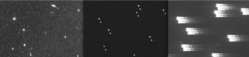
Using nod-and-shuffle (Glazebrook & Bland-Hawthorn 2001), two slits are milled for each target: one for the object and one for sky. We chose to nod in both the RA and Dec directions, instead of in the Dec direction only, as is usually done. In this way, if a bad column on the CCD affects data in one slit at a given wavelength, it will not affect the data in the other slit at the same wavelength. In hindsight, the horizontal nod led to non-negligible data reduction issues due to scattered light within the camera, and is not necessarily recommended. The first 23 (17%) of PRIMUS masks designed had slit widths of either 0.8″ or 1.0″ and slit lengths of 1.2″, with nods of 1.6″ in RA and 3.2″ in Dec and a charge shuffle of 8 pixels. For the bulk of the survey (the remaining 109 masks) these numbers were increased to a slit width of 1.0″ and a slit length of 1.6″ to increase the S/N in the data. The corresponding nods were 2.0″ in RA and 4.0″ in Dec, with a shuffle of 10 pixels. The corresponding area on the detector allowed for each object is two rectangles, each 140 by 20 pixels, shifted with respect to one another by 10 pixels in the RA direction. (Extracted spectra are 150 pixels in length; any overlap with a close neighbor will effectively reduce the spectra by 10 pixels at the blue end.) Figure 4 shows a small portion of imaging in one field, the corresponding slit assignment for one slitmask covering this area (essentially a zeroth-order calibration image), and the dispersed raw data.
Slitmasks typically have 2,500 targets per mask, including alignment stars, spectrophotometric standard stars, galaxy and AGN targets, and empty sky slits. We avoided regions around bright stars due to difficulties in defining targets and due to scattered light. For space-based target imaging in the COSMOS field, we used a smaller bright star mask. The typical number of primary targets per slitmask is 1,600 (note that objects can be observed on multiple slitmasks). Individual targets were allowed to be observed on multiple slitmasks, which often occurred as there are two masks per pointing. In our science fields, 21% of the slits were occupied by “repeat” observations of isolated galaxy and AGN targets that did not have collisions (see below).
Figure 5 shows the layout of an example PRIMUS slitmask in the XMM-LSS field. The grey circular region shows the usable portion of the IMACS field of view in f/2 mode; there is strong vignetting in the corners of the IMACS camera. Each of the colored points shows an object for which a slit was milled on this mask. The black squares mark the locations of alignment stars used to acquire the field. High-priority targets are selected first: primary galaxies are shown in blue and calibration F stars are shown in magenta. The mask is then filled with lower-priority galaxies, shown in yellow, and empty sky slits, shown in red, that are used in our data reduction. During mask design, we optimized slit positions for the local sidereal time (LST) of observation but always designed masks to have a position angle of 0 degrees.
6.2. Density-Dependent Sampling
When designing slitmasks one must take care to not have spectra of adjacent objects overlap on the detectors. The footprint of our spectra on the detectors corresponds to an area of on the sky, and thus any close pairs of galaxies can have only one galaxy of the pair observed on a given slitmask. Observing two slitmasks per pointing greatly alleviates this problem. However, galaxies to are sufficiently clustered in the plane of the sky that even with two slitmasks per pointing we would undersample the densest regions in a way that would be difficult to recover without modeling our completeness using simulations. To alleviate this issue, we employ a density-dependent sampling method in which objects with more neighbors are sparse-sampled. This strategy yields a primary sample in which each object has on average only one close neighbor (within the footprint on the sky). As these sampling rates are known for every object, we know the appropriate weight of each object in our primary sample that we do target. We can therefore recover unbiased two-point correlation functions and environmental statistics after applying the appropriate weights.
To calculate the targeting weight, we first divide the galaxy sample into two groups: group A contains the brighter galaxies to our “100% sampling limiting magnitude” (e.g., ) and group B contains galaxies 0.5 magnitude fainter (e.g., ). The number of potential collisions (objects whose spectra would overlap on the CCD) in the joint A+B sample is calculated for each galaxy in the sample. Any galaxy in group B that has more than two collisions is then sparse sampled at a rate of 30%. As discussed above, this sparse sampling (as a function of magnitude) is done to ensure that the fainter galaxies, which may have higher redshift incompleteness, do not dominate the assigned slits compared to the brighter galaxies.
After the sample of fainter galaxies has been sparse-sampled, we again count the number of potential collisions for every galaxy in the surviving A+B set. Then a density-dependent sampling probability is assigned, which depends on the number of collisions, where
| (7) |
where includes a self-count. Therefore, if , then both galaxies can be observed on separate slitmasks. Only if is a density-dependent sampling weight required.
Galaxies are then assigned to slitmasks using these probabilities, where every galaxy is given a random number between 0 and 1 such that if the random number is smaller than , then the target is assigned a slit. This sample of surviving density- and sparse-sampled objects is our primary sample. The random sampling is performed for each object, so it is possible that some collisions will remain after the subsampling. We use a numerator of 1.8 in equation 7 as a compromise between decreasing the number of surviving triplets (and hence improving completeness) and increasing the size of the primary sample. The advantage of the density-dependent a priori sampling is that most collisions are removed by a process with a well-defined sampling weight.
Using this algorithm we assign slits to 80% of galaxies to (or the equivalent “100% sampling limiting magnitude” in each field) and 96% of the density-dependent sample (the galaxies that passed the density-dependent sampling). As the sampling is done using well-defined weights which are tracked throughout the target selection process and the random seeds are saved, we can apply a “targeting” weight to each object in statistical analyses such as the correlation function or luminosity function, which will account for the fact that not all galaxies could be assigned slits.
7. Observations
The low-dispersion prism was commissioned in January 2006. PRIMUS slitmasks were observed during a total of 37 nights in a series of observing runs spanning two years, from March 2006 to January 2008, in blocks of two to seven nights with time allocated through Arizona, MIT, Harvard, Michigan, and NOAO. A total of 132 slitmasks were observed in science fields as well as 10 additional slitmasks in calibration fields.
Typical integration times for each slitmask were approximately one hour, with the exception of masks in the COSMOS field, which were observed for 1.5 hours to obtain higher S/N spectra and to target to a slightly fainter limiting magnitude. We observed in nod-and-shuffle mode, with 60 second dwell times, in sets of 16 (8 on, 8 off). We used the atmospheric dispersion corrector (ADC) on IMACS for all of our observations. Dome flats through the filters were taken in the afternoon, as well as twilight flats through the filters. Masks were aligned with typically two bright stars per CCD, for a total of 16 alignment stars. Alignment was often checked and corrected for, if needed, after half an hour of exposing. Arcs were taken during the night at the end of science exposures for each slitmask to facilitate wavelength calibration.
The seeing varied from FWHM″to ″, with typical values ″. The S/N of the data was monitored in real time by reducing bright objects on a portion of the mask; masks with low S/N were observed for longer periods of time or again on subsequent nights under better conditions.
8. Merging Photometry


Optical ground-based data in each of the PRIMUS fields was gathered not just for targeting purposes, but to use in fitting for redshifts and in deriving K-corrections (details are given in Cool et al., in preparation). When fitting for the redshift, the photometric data points are not upweighted relative to the spectroscopic data. Every pixel is weighted by its corresponding inverse variance, and each photometric band is treated as one pixel. The spectroscopic data therefore dominate the redshift fit.
Table 4 lists the optical imaging used in each field, in addition to the telescope and camera that it was taken with, as well as zeropoint offsets that were applied (details are given below), and the reference or source of the data. We adopt a minimum error floor to the photometry in each field, between 2%-10% in each band, which is used during redshift determination. For catalogs that were on the Vega system, we applied Vega-to-AB corrections as listed in the table. Catalogs that were on the AB system did not require corrections. Details of the GALEX, Spitzer, and X-ray data in our fields will be given elsewhere.
To test the relative calibration of the photometry in each field we selected stars with good photometry (i.e., unsaturated, high S/N) and constructed color-color diagrams using every combination of the available filters. We then compared the observed position of the stellar locus (corrected for Galactic reddening; Schlegel et al. 1998; O’Donnell 1994) to the locus predicted by the Pickles (1998) stellar library for metal-poor dwarfs (i.e., similar to stars in the Galactic halo; Ivezić et al. (2008) ). When synthesizing photometry we used the best-available filter curves in each field, convolved with the detector quantum efficiency, telescope throughput, and atmospheric transmission (see Table 4).
In several of our fields we found non-negligible systematic offsets between the observed and predicted stellar loci. To correct for these offsets, in the CDFS-SWIRE field we applied the recommended zeropoint corrections from Rowan-Robinson et al. (2008), in COSMOS we applied the offsets derived by Ilbert et al. (2009), and in our XMM-LSS field we used the Erben et al. (2009) recommended offsets. For the DEEP2 fields we adopted a different strategy. First, we retrieved PSF photometry of F stars observed by the SDSS in each field and applied the recommended absolute calibration offsets to the measured magnitudes.222See http://howdy.physics.nyu.edu/index.php/Kcorrect for a description of the absolute AB calibration of the SDSS photometry. We only considered stars with to ensure good measurements and to avoid saturation effects. We then fit the observed photometry with Kurucz (1993) models on a grid of metallicity, Teff, and (Lejeune et al. 1997) and computed synthetic magnitudes. Comparing the observed and synthetic photometry yielded the offsets listed in Table 4. Applying these various corrections to the photometry in each field led to excellent correspondence between the observed stellar locus, and the stellar locus predicted by the Pickles (1998) stellar library.
| \colrule\colruleBand | telescopeaaaCameras used at each telescope: CFHT is Megacam, except for the imaging in the DEEP2 fields, which is CFHT12k. CTIO is MOSAIC on the Blanco 4m, ESO-2.2m is WFI, MMT is Megacam, Subaru is Suprime-Cam, VLT is VIMOS. | zeropoint | min. | VegaAB | ref. | |
| offset | error | |||||
| \colrule\colrule CDFS-SWIRE | ||||||
| CTIO | 3672.0 | 0.049 | 0.05 | 0.708 | bbbLonsdale et al. (2003), http://www.astro.caltech.edu/bsiana/cdfs_opt | |
| CTIO | 4733.3 | -0.034 | 0.05 | -0.080 | bbbLonsdale et al. (2003), http://www.astro.caltech.edu/bsiana/cdfs_opt | |
| CTIO | 6243.0 | -0.095 | 0.05 | 0.168 | bbbLonsdale et al. (2003), http://www.astro.caltech.edu/bsiana/cdfs_opt | |
| CTIO | 7613.2 | -0.010 | 0.05 | 0.393 | bbbLonsdale et al. (2003), http://www.astro.caltech.edu/bsiana/cdfs_opt | |
| CTIO | 8932.3 | -0.030 | 0.05 | 0.531 | bbbLonsdale et al. (2003), http://www.astro.caltech.edu/bsiana/cdfs_opt | |
| \colrule CDFS-CALIB | ||||||
| ESO-2m | 3647.5 | 0.0 | 0.02 | 0.770 | ccfootnotemark: c | |
| ESO-2m | 4554.4 | 0.0 | 0.02 | -0.130 | ccfootnotemark: c | |
| ESO-2m | 5358.1 | 0.0 | 0.02 | -0.020 | ccfootnotemark: c | |
| ESO-2m | 6432.4 | 0.0 | 0.02 | 0.190 | ccfootnotemark: c | |
| ESO-2m | 8523.6 | 0.0 | 0.02 | 0.490 | ccfootnotemark: c | |
| \colrule COSMOS | ||||||
| CFHT | 3805.0 | -0.054 | 0.05 | 0.0 | ddfootnotemark: d | |
| Subaru | 4728.6 | -0.024 | 0.02 | 0.0 | eefootnotemark: e | |
| Subaru | 6249.1 | -0.003 | 0.02 | 0.0 | eefootnotemark: e | |
| CFHT | 7582.6 | 0.007 | 0.02 | 0.0 | ddfootnotemark: d | |
| Subaru | 7646.0 | -0.019 | 0.02 | 0.0 | eefootnotemark: e | |
| Subaru | 9011.0 | 0.037 | 0.02 | 0.0 | eefootnotemark: e | |
| \colrule DEEP2 - 23hr and 02hr | ||||||
| CFHT | 4402.0 | -0.011 | 0.05 | 0.0 | fffootnotemark: f | |
| CFHT | 6595.1 | -0.034 | 0.05 | 0.0 | fffootnotemark: f | |
| CFHT | 8118.7 | 0.035 | 0.05 | 0.0 | fffootnotemark: f | |
| CFHT | 7659.1 | 0.015 | 0.05 | 0.0 | ggfootnotemark: g | |
| CFHT | 8820.9 | 0.025 | 0.05 | 0.0 | ggfootnotemark: g | |
| \colrule | ||||||
| \colrule\colruleBand | telescopeaaaCameras used at each telescope: CFHT is Megacam, except for the imaging in the DEEP2 fields, which is CFHT12k. CTIO is MOSAIC on the Blanco 4m, ESO-2.2m is WFI, MMT is Megacam, Subaru is Suprime-Cam, VLT is VIMOS. | zeropoint | min. | VegaAB | ref. | |
| offset | error | |||||
| \colrule\colrule DEEP2 - 02hr | ||||||
| MMT | 3604.1 | -0.087 | 0.05 | 0.0 | hhfootnotemark: h | |
| MMT | 4763.5 | 0.079 | 0.05 | 0.0 | hhfootnotemark: h | |
| MMT | 7770.5 | -0.036 | 0.05 | 0.0 | hhfootnotemark: h | |
| \colrule DLS | ||||||
| CTIO | 4382.0 | 0.0 | 0.05 | -0.080 | iifootnotemark: i | |
| CTIO | 5398.8 | 0.0 | 0.05 | 0.012 | iifootnotemark: i | |
| CTIO | 6501.5 | 0.0 | 0.05 | 0.212 | iifootnotemark: i | |
| CTIO | 8966.4 | 0.0 | 0.05 | 0.000 | iifootnotemark: i | |
| \colrule ELAIS-S1 | ||||||
| ESO-2m | 4344.1 | 0.0 | 0.05 | -0.090 | jjfootnotemark: j | |
| ESO-2m | 5455.6 | 0.0 | 0.05 | 0.020 | jjfootnotemark: j | |
| ESO-2m | 6441.6 | 0.0 | 0.05 | 0.206 | jjfootnotemark: j | |
| VLT | 8086.3 | 0.0 | 0.10 | 0.456 | kkfootnotemark: k | |
| \colrule SDSS | ||||||
| APO-2.5m | 3546.0 | -0.04 | 0.05 | 0.0 | llfootnotemark: l | |
| APO-2.5m | 4669.6 | 0.01 | 0.02 | 0.0 | llfootnotemark: l | |
| APO-2.5m | 6156.2 | 0.01 | 0.02 | 0.0 | llfootnotemark: l | |
| APO-2.5m | 7471.6 | 0.03 | 0.02 | 0.0 | llfootnotemark: l | |
| APO-2.5m | 8917.4 | 0.04 | 0.03 | 0.0 | llfootnotemark: l | |
| \colrule XMM-LSS and VVDS | ||||||
| CFHT | 3805.0 | -0.10 | 0.05 | 0.0 | ddfootnotemark: d | |
| CFHT | 4824.0 | -0.02 | 0.02 | 0.0 | ddfootnotemark: d | |
| CFHT | 6199.7 | -0.05 | 0.02 | 0.0 | ddfootnotemark: d | |
| CFHT | 7582.6 | -0.05 | 0.02 | 0.0 | ddfootnotemark: d | |
| CFHT | 8793.0 | -0.05 | 0.02 | 0.0 | ddfootnotemark: d | |
| \colrule | ||||||
Wolf et al. (2004) ddfootnotemark: dCFHTLS T0003 release eefootnotemark: eCapak et al. (2007) fffootnotemark: fCoil et al. (2004) ggfootnotemark: gL. Lin, private communication, lihwailin@asiaa.sinica.edu.tw hhfootnotemark: hM. Ashby, private communication, mashby@cfa.harvard.edu iifootnotemark: iWittman et al. (2006) jjfootnotemark: jBerta et al. (2006) kkfootnotemark: kBerta et al. (2008) llfootnotemark: lAbazajian et al. (2009)
9. Data Summary
A summary of the number of objects observed by PRIMUS, and the number with robust redshifts, is given in Table 1. PRIMUS observed a total of 132 slitmasks in our science fields, covering 9.1 deg2, most of which has multi-wavelength coverage from Spitzer, GALEX, XMM or Chandra. The fraction of objects to the “100% targeting magnitude limit” that were observed is very high, 80%. Of the total 270,000 objects targeted to , we obtain robust redshifts for 130,000 unique sources, 90,000 of which are galaxies and AGN in the primary sample. Our redshift success rate of 50% to our full targeting depth of i23.5 is roughly comparable to spectroscopic surveys of similar depth; in DEEP2 the redshift success fraction is 65% and in the first epoch VVDS data it is 80% for “flag 2, 3, 4 or 9” sources, which have a similar redshift quality as our robust (; see below) redshifts here. The redshift success rate of PRIMUS is a function of S/N of the spectrum, which closely correlates with galaxy magnitude. At bright magnitudes () the redshift success rate is 90% and it falls to 70% at , with little dependence on apparent galaxy color. A detailed discussion of the dependence of the redshift success fraction on magnitude and color will be presented in Cool et al. (in preparation) and Moustakas et al. (in preparation).
Example spectra are shown in Figure 6. The resolution of PRIMUS is high enough to allow us to distinguish broad-line AGN (lower panel) from emission line galaxies (middle panel) and to identify continuum features such as the 4000 Å break in early-type galaxies (top panel). However, it is generally not high enough to measure stellar velocity dispersions, emission-line widths, or the strengths of low equivalent width nebular (narrow) lines.
The data reduction and redshift fitting pipelines are described in Cool et al. (in preparation). Briefly, we determine redshifts by fitting the observed spectra and multiwavelength photometry simultaneously with an empirical library of galaxy spectral templates on a coarse redshift grid in the range . For each object, we construct the redshift probability distribution function, , by marginalizing over the galaxy templates and identify the first several maxima. We then refine our search on a finer grid centered on the most likely redshift (i.e., the mode of ) and compute the final redshift and uncertainty, and , as the first and second moments of the refined distribution.
To assess the confidence level of our redshift measurement, we compute a statistic , where is the difference between the first and second minima (maxima) of the () distribution. In effect, is proportional to the narrowness of the distribution around the first maximum and inversely proportional to the relative probability between the two most likely redshifts. Small values of imply a sharply peaked, unimodal distribution, while a distribution with a broad maximum or with a potentially significant second maximum result in large values of .
Using our spectroscopic calibration fields, we correlate with both the cumulative fraction in which PRIMUS measures the “correct” high-resolution redshift (i.e., ) and with the outlier rate, corresponding to the fraction of objects with at a given . We then associate three intervals of the continuous variable with our redshift confidence flag, , such that we maximize the fraction of correct redshifts and minimize the outlier rate.
We also fit each spectrum with a custom suite of AGN templates in the range and with stellar templates drawn from the Pickles (1998) stellar library spanning a wide range of spectral types. We use the differences between the various minima to select among the galaxy, AGN, and stellar templates, with some empirically motivated modifications; see Cool et al. (in preparation), for details.
Figure 7 shows the redshift distributions of PRIMUS galaxies (left panel) and broad-line AGN (right panel). In each figure the solid line shows the redshifts distribution for the full sample and the dashed line for the primary sample. The mean redshift of the survey is .
Figure 8 compares the PRIMUS redshift to a high resolution spectroscopic redshift for sources from either DEEP2, VVDS, or zCOSMOS in our calibration fields. Shown are redshifts for a sample of galaxies with and magnitude in the DEEP2 fields or in the VVDS and zCOSMOS fields. In order to match the observed redshift distribution of sources in the full PRIMUS sample, for this comparison we downweight sources in the DEEP2 fields so as to create a comparable sample with a similar median redshift as our survey. We use only the most robust redshifts from zCOSMOS and VVDS (flag 3 and 4). For each redshift confidence flag, Q, we list the fraction of sources with and with , the redshift accuracy , (where we quote the normalised median absolute deviation, defined as 1.48 median(), and the number of objects with each confidence flag. Objects with a PRIMUS redshift confidence of Q2 are shown in the upper left panel; these sources have =0.036 and we do not consider these sources to have a “robust” redshift. Objects with Q3 are shown in the upper right; these sources have a robust redshift but a higher dispersion than the Q4 sources shown in the lower left. For most science purposes we will use samples with Q3, shown in the lower right panel. The Q4 sample is the purest, with the greatest redshift accuracy and lowest outlier rate, while the Q3 sample is somewhat larger. The redshift accuracy of the Q4 sample is =0.0043, while the accuracy of the Q3 sample is =0.0051. The outlier rate of objects in this sample with is 8% for Q3 and 3% for Q4, while the outlier rate with is 2% for Q3 and 1% for Q4.
The outlier rate varies slightly between fields, depending on the optical photometric bands available, in particular the band. For the vast majority of the sample (90% of our sources), the best fit redshift did not change if the photometric data was or was not used. Including the photometric data helped for only 10% of the objects; these are sources where there is a degeneracy between the Balmer break and the presence of O[II] 3727 Å in our low-dispersion spectra. For these sources the inclusion of photometric data, band in particular, helped to break the degeneracy and the redshift changed by up to 8% in . Details are given in Cool et al. (in preparation).
As an independent check of the redshift precision, Wong et al. (2010) identify close galaxy pairs in PRIMUS within a projected separation of kpc on the plane of the sky and examine the redshift differences between the pairs. They find that 90% of the pair galaxies are separated from their close neighbor by . As almost all galaxies that are this close on the plane of the sky are physically associated (i.e., in the same dark matter halo), the pair galaxies should be at the same redshift modulo peculiar velocities along the line of sight. Therefore the distribution of the redshift differences between close pairs is a strong test of our redshift precision, completely independent of comparisons against high resolution redshifts.
Figure 9 shows the absolute magnitude versus redshift for 116,041 PRIMUS sources between . Restframe magnitudes are computed using the kcorrect software package (Blanton & Roweis 2007), which fits the sum of a set of basis templates at the PRIMUS redshift to the broadband optical photometry available in each field. The basis templates are based on stellar population synthesis models and are constrained to produce a non-negative best-fit template, which is used to estimate the restframe absolute magnitude from the nearest available observed photometric band.
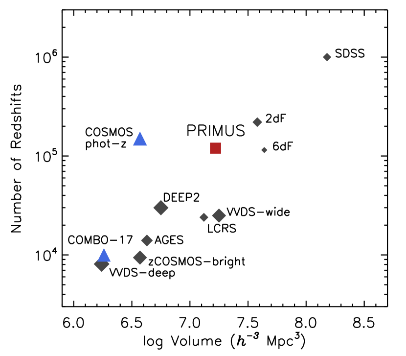
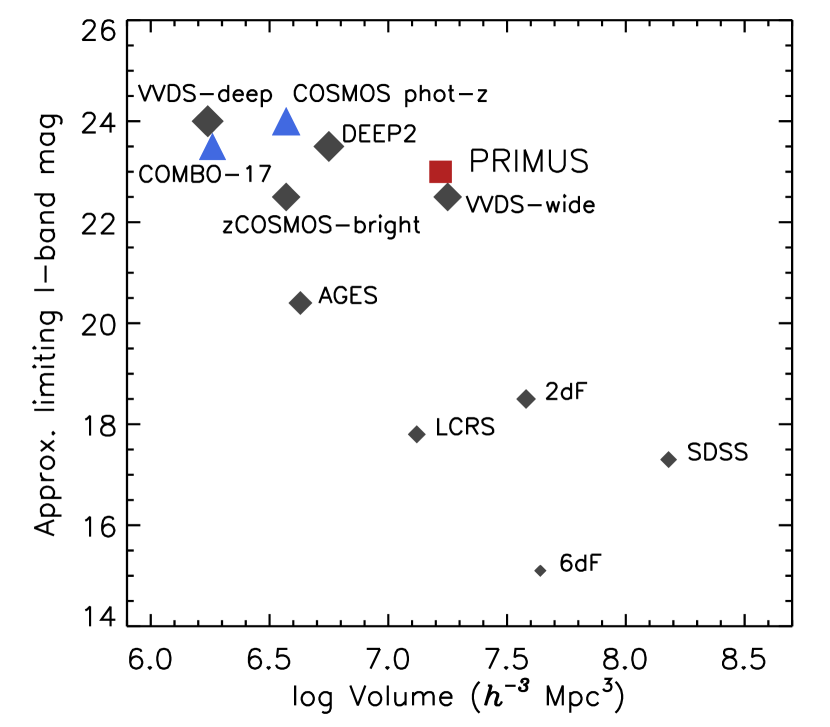
Figure 10 compares PRIMUS to other flux-limited galaxy redshift surveys, in terms of the number of objects, volume, and approximate limiting magnitude of the survey. At lower redshifts, we compare to 2dFGRS (Colless et al. 2001), 6dF (Jones et al. 2009), LCRS (Shectman et al. 1996), and SDSS (York et al. 2000). At higher redshifts we compare to AGES, DEEP2 (Davis et al. 2003, 2007), COMBO-17 (Wolf et al. 2003, 2004), VVDS (Le Fèvre et al. 2005; Garilli et al. 2008), and zCOSMOS (Lilly et al. 2007), as well as the COSMOS 30-band photometric redshifts (Ilbert et al. 2009). In this comparison we use the number of unique objects with robust redshifts for each survey. For SDSS we compare to the main flux-limited galaxy sample and do not include the luminous red galaxy sample. For ongoing surveys (VVDS-Wide, zCOSMOS-bright) we show the projected final numbers with a correction based on the fraction of robust redshifts (flag 2, 3, 4 or 9) in the current release. We limit the PRIMUS data to , which covers a volume of . In the right panel of Figure 10 we compare the various redshift surveys in terms of volume and depth, where we have plotted the IAB-band limiting magnitude or an approximate equivalent for surveys limited in other bands. PRIMUS is the largest-volume, intermediate-redshift spectroscopic galaxy redshift survey undertaken to date. The VVDS-wide survey (Garilli et al. 2008) is the only other survey covering a comparable volume at these redshifts, though it is half a magnitude shallower and has a sample size that is 30% that of PRIMUS. As we show here, PRIMUS requires a similar amount of total telescope time as the COSMOS 30-band photometric redshift survey, but PRIMUS covers 5 times as much area with comparable redshift precision.
The PRIMUS survey will allow for the most robust measurements of galaxy properties and large-scale structure to performed to date. Initial studies include quantifying triggered star formation in close galaxy pairs (Wong et al. 2010), studying obscured star formation on the red sequence (Zhu et al. 2010), and measuring the luminosity functions (Cool et al., in preparation) and stellar mass functions (Moustakas et al., in preparation) of star-forming and quiescent galaxies. The PRIMUS redshift precision of 0.5% allows for clustering and environment studies, which integrate over that amount in redshift space due to peculiar velocities of galaxies within overdense regions. With PRIMUS we will be able to measure the galaxy luminosity function, SFR, and stellar mass density as a function of environment to with low cosmic variance errors. PRIMUS will also lead to more precise determinations of correlation functions for galaxies and AGN at intermediate redshifts than has been previously measured, due to the large survey volume spread across multiple fields on the sky.
We will present the data reduction, redshift fitting, redshift confidence and precision, and survey completeness for PRIMUS in Cool et al. (in preparation), to which we refer the reader for additional details about the survey.
References
- Abazajian et al. (2009) Abazajian, K. N., et al. 2009, ApJS, 182, 543
- Adami et al. (2010) Adami, C., et al. 2010, A&A, 509, A260000+
- Ashby et al. (2009) Ashby, M. L. N., et al. 2009, ApJ, 701, 428
- Berta et al. (2006) Berta, S., et al. 2006, A&A, 451, 881
- Berta et al. (2008) —. 2008, A&A, 488, 533
- Bigelow & Dressler (2003) Bigelow, B. C., & Dressler, A. M. 2003, Proc. SPIE, 4841, 1727
- Blanton & Roweis (2007) Blanton, M. R., & Roweis, S. 2007, AJ, 133, 734
- Brodwin et al. (2006) Brodwin, M., et al. 2006, ApJ, 651, 791
- Budavari et al. (2003) Budavari, T., et al. 2003, ApJ, 595, 59
- Capak et al. (2007) Capak, P., et al. 2007, ApJS, 172, 99
- Coil et al. (2004) Coil, A. L., et al. 2004, ApJ, 617, 765
- Colless et al. (2001) Colless, M., et al. 2001, MNRAS, 328, 1039
- Coupon et al. (2009) Coupon, J., et al. 2009, A&A, 500, 981
- Davis et al. (1982) Davis, M., Huchra, J., Latham, D. W., & Tonry, J. 1982, ApJ, 253, 423
- Davis et al. (2003) Davis, M., et al. 2003, Proc. SPIE, 4834, 161
- Davis et al. (2007) Davis, M., et al. 2007, ApJ, 660, 1
- Eisenhardt et al. (2004) Eisenhardt, P. R., et al. 2004, ApJS, 154, 48
- Erben et al. (2009) Erben, T., et al. 2009, A&A, 493, 1197
- Furusawa et al. (2008) Furusawa, H., et al. 2008, ApJS, 176, 1
- Garilli et al. (2008) Garilli, B., et al. 2008, A&A, 486, 683
- Giacconi et al. (2001) Giacconi, R., et al. 2001, ApJ, 551, 624
- Gladders & Yee (2005) Gladders, M. D., & Yee, H. K. C. 2005, ApJS, 157, 1
- Glazebrook & Bland-Hawthorn (2001) Glazebrook, K., & Bland-Hawthorn, J. 2001, PASP, 113, 197
- Hamilton & Tegmark (2004) Hamilton, A. J. S., & Tegmark, M. 2004, MNRAS, 349, 115
- Ilbert et al. (2009) Ilbert, O., et al. 2009, ApJ, 690, 1236
- Ivezić et al. (2008) Ivezić, Ž., et al. 2008, ApJ, 684, 287
- Jones et al. (2009) Jones, D. H., et al. 2009, MNRAS, 399, 683
- Koekemoer et al. (2007) Koekemoer, A. M., et al. 2007, ApJS, 172, 196
- Kurucz (1993) Kurucz, R. L. 1993, CD-ROM 13, ATLAS9 Stellar Atmosphere Programs and 2 km/s Grid (Cambridge: Smithsonian Astrophys. Obs.)
- Lawrence et al. (2007) Lawrence, A., et al. 2007, MNRAS, 379, 1599
- Le Fèvre et al. (2005) Le Fèvre, O., et al. 2005, A&A, 439, 845
- Lejeune et al. (1997) Lejeune, T., Cuisinier, F., & Buser, R. 1997, A&AS, 125, 229
- Lilly et al. (2007) Lilly, S. J., et al. 2007, ApJS, 172, 70
- Liu et al. (2008) Liu, F., et al. 2008, Proc. SPIE, 7017, 16
- Lonsdale et al. (2003) Lonsdale, C. J., et al. 2003, PASP, 115, 897
- Martin et al. (2005) Martin, D. C., et al. 2005, ApJ, 619, L1
- Mobasher et al. (2004) Mobasher, B., et al. 2004, ApJ, 600, L167
- O’Donnell (1994) O’Donnell, J. E. 1994, ApJ, 422, 158
- Oliver et al. (2000) Oliver, S., et al. 2000, MNRAS, 316, 749
- Padmanabhan et al. (2005) Padmanabhan, N., et al. 2005, MNRAS, 359, 237
- Pelló et al. (2009) Pelló, R., et al. 2009, A&A, 508, 1173
- Pickles (1998) Pickles, A. J. 1998, PASP, 110, 863
- Pierre et al. (2004) Pierre, M., et al. 2004, Journal of Cosmology and Astroparticle Physics, 9, 11
- Quadri et al. (2007) Quadri, R., et al. 2007, AJ, 134, 1103
- Ravikumar et al. (2007) Ravikumar, C. D., et al. 2007, A&A, 465, 1099
- Richards et al. (2004) Richards, G. T., et al. 2004, ApJS, 155, 257
- Rowan-Robinson et al. (2008) Rowan-Robinson, M., et al. 2008, MNRAS, 386, 697
- Sanders et al. (2007) Sanders, D. B., et al. 2007, ApJS, 172, 86
- Schlegel et al. (1998) Schlegel, D. J., Finkbeiner, D. P., & Davis, M. 1998, ApJ, 500, 525
- Shectman et al. (1996) Shectman, S. A. et al. 1996, ApJ, 470, 172
- Skrutskie et al. (1997) Skrutskie, M. F., et al. 1997, in Astrophysics and Space Science Library, Vol. 210, The Impact of Large Scale Near-IR Sky Surveys, ed. F. Garzon, N. Epchtein, A. Omont, B. Burton, & P. Persi, 25
- Steidel et al. (2004) Steidel, C. C., et al. 2004, ApJ, 604, 534
- Swanson et al. (2008) Swanson, M. E. C., et al. 2008, MNRAS, 387, 1391
- van Dokkum et al. (2009) van Dokkum, P. G., et al. 2009, PASP, 121, 2
- Wittman et al. (2006) Wittman, D., et al. 2006, ApJ, 643, 128
- Wittman et al. (2002) Wittman, D. M., et al. 2002, Proc. SPIE, 4836, 73
- Wolf et al. (2003) Wolf, C., et al. 2003, A&A, 401, 73
- Wolf et al. (2004) —. 2004, A&A, 421, 913
- Wong et al. (2010) Wong, K., et al. 2011, ApJ, 728, 119
- York et al. (2000) York, D. G., et al. 2000, AJ, 120, 1579
- Zhu et al. (2010) Zhu, G., et al. 2011, ApJ, 726, 110