A Coverage Study of the CMSSM Based on ATLAS Sensitivity Using Fast Neural Networks Techniques

Abstract:

We assess the coverage properties of confidence and credible intervals on the CMSSM parameter space inferred from a Bayesian posterior and the profile likelihood based on an ATLAS sensitivity study. In order to make those calculations feasible, we introduce a new method based on neural networks to approximate the mapping between CMSSM parameters and weak-scale particle masses. Our method reduces the computational effort needed to sample the CMSSM parameter space by a factor of $\sim 10^{4}$ with respect to conventional techniques. We find that both the Bayesian posterior and the profile likelihood intervals can significantly over-cover and identify the origin of this effect to physical boundaries in the parameter space. Finally, we point out that the effects intrinsic to the statistical procedure are conflated with simplifications to the likelihood functions from the experiments themselves.

1 Introduction

Experiments at the Large Hadron Collider (LHC) will soon start testing many models of particle physics beyond the Standard Model (SM). Particular attention will be given to the Minimal Supersymmetric SM (MSSM) and other scenarios involving softly-broken supersymmetry (SUSY).

We are interested in the statistical properties of the emerging methodology used to infer the parameters of these models. Here we consider a restricted class of SUSY models with certain universality assumptions regarding the SUSY breaking parameters. This scenario is commonly called mSUGRA or the Constrained Minimal Supersymmetric Standard Model (CMSSM) [1, 2]. The model is defined in terms of five free parameters: common scalar ($m_{0}$), gaugino ($m_{1/2}$) and tri–linear ($A_{0}$) mass parameters (all specified at the GUT scale) plus the ratio of Higgs vacuum expectation values $\tan\beta$ and $\text{sign}(\mu)$, where $\mu$ is the Higgs/higgsino mass parameter whose square is computed from the conditions of radiative electroweak symmetry breaking (EWSB).

A common procedure to explore the model’s parameter space consisted of evaluating the likelihood function on a fixed grid, often encompassing only 2 or 3 dimensions at the time [3, 4, 5, 6, 7, 8]. Of course, the number of likelihood evaluations in a grid scan scales exponentially with the dimensionality of the parameter space, making it impractical for a full exploration of the CMSSM parameter space. More recently new approaches based on both Frequentist and Bayesian statistics coupled with Markov Chain Monte Carlo (MCMC) methodology have been applied [9, 10, 11, 12, 13, 14, 15, 16, 17, 18, 19, 20]. The efficiency of the MCMC techniques allow for a full exploration of multidimensional models. However, the likelihood function of these models is complex, multimodal with many narrow features, making the exploration task with conventional MCMC methods challenging often with low sampling efficiency.

More recently, a novel scanning algorithm, called MultiNest [21, 22, 23], has been proposed in the Bayesian context. It is based on the framework of Nested Sampling, recently invented by Skilling [24]. MultiNest has been developed in such a way as to be an extremely efficient sampler of the posterior distribution even for likelihood functions defined over a parameter space of large dimensionality with a very complex structure. It has been applied for the exploration of several models within the MSSM [25, 23, 26, 27, 28, 29, 30, 31, 32] and its minimal extension, the so–called Next-to-Minimal Supersymmetric SM (NMSSM) [33]. Nested sampling has also been shown as a powerful technique for model reconstruction based on LHC data [34].

Having implemented sophisticated statistical and scanning methods, several groups have turned their attention to evaluating the sensitivity to the choice of priors [15, 35, 23] and of scanning algorithms [36]. Those analyses indicate that current constraints are not strong enough to dominate the posterior and that the choice of prior does influence the resulting inference. While confidence intervals derived from the profile likelihood or a chi-square have no formal dependence on a prior, there is a sampling artifact when the contours are extracted from samples produced from MCMC or MultiNest [23].

Given the sensitivity to priors and the differences between the intervals obtained from different methods, it is natural to seek out a quantitative assessment of their performance. A natural quantity for this evaluation is coverage: the probability that an interval will contain (cover) the true value of a parameter. The defining property of a 95% confidence interval is that the procedure that produced it should produce intervals that cover the true value 95% of the time; thus, it is reasonable to check if the procedures have the properties they claim. Coverage is a frequentist concept: one assumes the true parameters take on some specific, unknown values and considers the outcome of repeated experiments. Intervals based on Bayesian techniques are meant to contain a given amount of posterior probability for a single measurement and are referred to as credible intervals to make clear the distinction. While Bayesian techniques are not designed with coverage as a goal, it is still meaningful to investigate their coverage properties. In fact, the development of Bayesian methods with desirable frequentist properties is an active area of research for professional statisticians [37, 38]. Moreover, the frequentist intervals obtained from the profile likelihood or chi-square functions are based on asymptotic approximations and are not guaranteed to have the claimed coverage properties.

In this work we study the coverage properties of both Bayesian and Frequentist procedures commonly used to study the CMSSM. In particular, we consider the coverage of the ATLAS “SU3” CMSSM benchmark point. The task requires extensive computational expenditure, which would be unfeasible with standard analysis techniques. Thus in this paper we explore the use of a class of machine learning devices called Artificial Neural Networks (ANNs) to approximate the most computationally intensive sections of the analysis pipeline. Such techniques have been successfully employed before in the cosmological setting to accelerate inference massively [39]. Within particle physics, ANNs have been used extensively for event classification, but we are not aware of their use in approximating the mapping between fundamental Lagrangian parameters and observable quantities such as a mass spectrum.

This paper will be arranged as follows: in Section 2 we will briefly review the Bayesian methodology and the CMSSM framework that this work operates within while in Section 3 we will outline the use of neural networks to approximate SUSY spectrum calculators. In Section 3.1 we will demonstrate our method, discuss the accuracy of our network predictions against the dedicated spectrum calculator, and demonstrate computational performance improvements. In Section 4 we present the results of a coverage study employing the trained networks. We conclude with a discussion in Section 5.

2 Statistical framework and supersymmetry model

The cornerstone of Bayesian inference is Bayes’ Theorem, which reads

$$p(\Theta|d)=\frac{p(d|\Theta)p(\Theta)}{p(d)}.$$ (1)

The quantity $p(\Theta|d)$ on the l.h.s. of eq. (1) is called the posterior, while on the r.h.s., the quantity $p(d|\Theta)$ is the likelihood (when taken as a function $\Theta$ for fixed data, $d$). The quantity $p(\Theta)$ is the prior which encodes our state of knowledge about the values of the parameters $\Theta$ before we see the data. The state of knowledge is then updated to the posterior via the likelihood. Finally, the quantity in the denominator is called evidence or model likelihood. If one is interested in constraining the model’s parameters, the evidence is merely a normalization constant, independent of $\Theta$, and can therefore be dropped (for further details, see e.g. [40]).

We denote the parameter set of the CMSSM introduced above ($m_{0}$, $m_{1/2}$, $A_{0}$ and $\tan\beta$) by $\theta$ (we fix sgn($\mu$) to be positive, motivated by arguments of consistency with the measured anomalous magnetic moment of the muon), while $\psi$ denotes the “nuisance parameters” whose values we are not interested in inferring, but which enter the calculation of the observable quantities. Here, the relevant nuisance parameters are the SM quantities

$$\psi\equiv\{M_{t},m_{b}(m_{b})^{\overline{MS}},\alpha_{s}(M_{Z})^{\overline{MS}},\alpha_{\text{em}}(M_{Z})^{\overline{MS}}\}\,,$$ (2)

where $M_{t}$ is the pole top quark mass, $m_{b}(m_{b})^{\overline{MS}}$ is the bottom quark mass at $m_{b}$, while $\alpha_{\text{em}}(M_{Z})^{\overline{MS}}$ and $\alpha_{s}(M_{Z})^{\overline{MS}}$ are the electromagnetic and the strong coupling constants at the $Z$ pole mass $M_{Z}$, the last three evaluated in the $\overline{MS}$ scheme. Note that there are no nuisance parameters associated with experimentally related systematics, which would instead be anticipated to be the case in future inference problems based on the results of LHC experiments. We denote the full 8–dimensional set of parameters by

$$\Theta=(\theta,\psi).$$ (3)

The likelihood evaluation in a SUSY particle model analysis involves the computation of the mass spectrum. It implies the use of an iterative procedure in which the renormalization group equations (RGEs) are solved. The current public numerical codes reach a precision at the level of a few percent in computing the spectrum [41]. For it, the RGEs are implemented up two-loop level and the calculation of the physical masses involve the inclusion, at least, of the full one-loop radiative corrections. The typical running time for the spectrum calculator is a few seconds per model point, which can seriously hinder all Monte-Carlo style explorations of the parameter space where $10^{5}-10^{7}$ parameter points need to be examined. In addition these parameter spaces have a unphysical regions which emit tachyonic solutions and/or in which EWSB is not fulfilled. Figure 1 illustrates that these regions can be evenly spread across some projections of the $\theta$ parameter space. Testing and discarding these unphysical points leads to large timing inefficiencies in the scan.

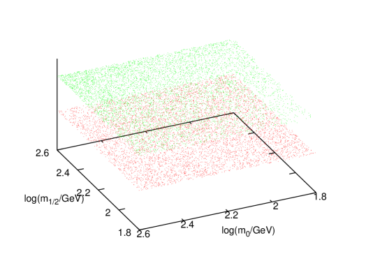
Figure 1: Physical (upper) and unphysical (lower) samples in $m_{0}-m_{1/2}$ space.

3 Approximating the spectrum calculators with neural networks

Any analysis of the CMSSM parameter space must relate the high-scale parameters $\theta$ with observable quantities, such as the sparticle mass spectrum at the LHC. As described above, this is achieved by evolving the RGEs, which is a computationally intensive procedure. We use SoftSusy [42] for calculating the sparticle mass spectrum, and denote the predicted weak-scale sparticle masses by $m$. One can view the RGEs simply as a mapping from $\Theta\to{\mbox{\boldmath$m$}}$, and attempt to engineer a computationally efficient representation of the function. There is a vast literature for multivariate function approximation, which includes techniques such as neural networks [43], radial basis functions [44], support vector machines [45], and regression trees [46, 47].

Here we use a multilayer perceptron (MLPs), a type of feed-forward neural network. We restrict ourselves to three-layer MLPs, which consist of an input layer ($\Theta_{l}$), a hidden layer ($h_{j}$), and an output layer ($y_{i}$). In such a network, the value of the nodes in the hidden and output layers are given by

hidden layer: $$h_{j}=g^{(1)}(f_{j}^{(1)}); f_{j}^{(1)}=\sum_{l}w^{(1)}_{jl}\Theta_{l}+\xi_{j}^{(1)},$$ (4)

output layer: $$y_{i}=g^{(2)}(f_{i}^{(2)}); f_{i}^{(2)}=\sum_{j}w^{(2)}_{ij}h_{j}+\xi_{i}^{(2)},$$ (5)

where the index $l$ runs over input nodes, $j$ runs over hidden nodes and $i$ runs over output nodes. The functions $g^{(1)}$ and $g^{(2)}$ are called activation functions and are chosen to be bounded, smooth and monotonic. The non-linear nature of the former is a key ingredient in constructing a viable network; we use $g^{(1)}(x)=\tanh x$ and $g^{(2)}(x)=x$.

The weights $w$ and biases $\xi$ are the quantities we wish to determine, which we denote collectively by $a$. As these parameters vary, a very wide range of non-linear mappings between the inputs and outputs are possible. In fact, according to a ‘universal approximation theorem’ [48, 49], a standard multilayer feed-forward network with a locally bounded piecewise continuous activation function can approximate any continuous function to any degree of accuracy if (and only if) the network’s activation function is not a polynomial and the network contains an adequate number of hidden nodes. This result applies when activation functions are chosen a priori and held fixed if $a$ is allowed to vary. In practice, one often must empirically find a network architecture with a suitable balance of training requirements, generalization, and prediction accuracy.

Table 1: Parameter ranges chosen for CMSSM parameters $\theta$ and nuisance parameters $\psi$. We have adopted uniform priors on the variables and ranges shown here.

CMSSM parameters: $\theta$

$\log(50)$ $<$ $\log m_{0},\log m_{1/2}$ (GeV) $<$ $\log(500)$

$-4$ $<$ $A_{0}$ (TeV) $<$ $4$

$2$ $<$ $\tan\beta$ $<$ $62$

SM nuisance parameters: $\psi$

$3.92$ $<$ $M_{t}$ $<$ $4.48$

$163.7$ $<$ $m_{b}(m_{b})^{\overline{MS}}$ $<$ $178.1$

$0.1096$ $<$ $\alpha_{em}(M_{Z})^{\overline{MS}}$ $<$ $0.1256$

$127.846$ $<$ $\alpha_{s}(M_{Z})^{\overline{(}MS)}$ $<$ $127.99$

3.1 Network training, accuracy, and performance

The procedure of adjusting the weights and biases of a network (and sometimes the architecture of the network itself) as to approximate the SoftSusy mapping is referred to as training, and requires the use of sophisticated algorithms. The training procedure is usually cast as an optimization problem with respect to some loss function $\mathcal{L}$. A training data set $\mathcal{D}=\{{\Theta}^{(k)},{\mbox{\boldmath$m$}}^{(k)}\}$ was used for this procedure, where $k$ is an index for input-output pairs generated with SoftSusy. The training dataset was typically chosen to have a few thousand points for this application. If the training sample adequately represents the function over the chosen region and the network has good generalization capabilities, then the trained network should approximate the function well on an independent testing sample. Below we describe the training algorithm and assess its accuracy with an independent testing sample.

Any training process requires the quantification of errors between the network outputs $y_{i}$ and the corresponding values from the training via some loss function. In this application we chose a simple squared error objective function in the network parameters $a$:

$$\mathcal{L}(\mathcal{D}|{\mbox{\boldmath$a$}})={\textstyle\frac{1}{2}}\sum_{k}\sum_{i}\left[m^{(k)}_{i}-y_{i}(\Theta^{(k)};{\mbox{\boldmath$a$}})\right]^{2}.$$ (6)

This is a highly non-linear, multi-modal function in hundreds or thousands of dimensions.

The problem of network training is analogous to one of parameter estimation in $a$ with Equation (6) playing the role of the log-likelihood function. For small networks this function can be adequately optimised using a form of gradient descent described as back propagation [50]. A complete Bayesian framework for the training of neural networks has been given by [51]. In this context the log of the posterior probability of $a$ given the training data $\mathcal{D}$ is:

$$\ln P({\mbox{\boldmath$a$}}|\mathcal{D})\propto-\mathcal{L}(\mathcal{D}|{\mbox{\boldmath$a$}})+\ln\Pi({\mbox{\boldmath$a$}})$$ (7)

where $\Pi$ is a prior distribution of the network parameters $a$. While it is conceptually feasible to use conventional Monte Carlo sampling based methods such as Metropolis-Hastings or Nested Sampling to optimise this function and thus recover the optimal set of $a$, the computational expense of this approach would be prohibitively high. In this work we have used an optimising suite of software called MemSys based on the principle of Maximum Entropy.

The MemSys algorithm chooses a positive-negative entropy function $S$ as the prior distribution, $\Pi({\mbox{\boldmath$a$}})$ with a hyperparameter $\alpha$ which controls the relative balance between prior and likelihood within the posterior distribution [52] so that Equation (7) becomes:

$$\ln P({\mbox{\boldmath$a$}}|\mathcal{D})\propto-\mathcal{L}(\mathcal{D}|{\mbox{\boldmath$a$}})+\alpha\ln S({\mbox{\boldmath$a$}}).$$ (8)

For each choice of $\alpha$ there is a set of network parameters $\hat{{\mbox{\boldmath$a$}}}$ that maximises the posterior distribution. As $\alpha$ is varied one obtains a path of maximum posterior solutions $\hat{{\mbox{\boldmath$a$}}}(\alpha)$ called the maximum-entropy trajectory. The MemSys algorithm begins the exploration of the joint distribution of $a$ and $\alpha$ by slowly introducing the likelihood term in the posterior with initially large values of $\alpha$. For each sampled value of $\alpha$ the algorithm converges to the maximum posterior solution $\hat{{\mbox{\boldmath$a$}}}$ via conjugate gradient descent. The parameter $\alpha$ is then slowly reduced via a rate parameter such that the new maximum entropy solution $\hat{{\mbox{\boldmath$a$}}}^{\prime}$ lies close to the previous solution $\hat{{\mbox{\boldmath$a$}}}$, thus ensuring a smooth descent to the optimal point in $a$ and $\alpha$. MemSys then returns an estimate of the maximum posterior network weights and biases. For more complete details of the MemSys algorithm we refer the reader to [53].

(a) $m_{\nu}^{1}$

(b) $m_{\nu}^{2}$

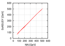
(c) $m_{se}^{R}$

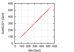
(d) $m_{se}^{L}$

(e) $m_{s\mu}^{R}$

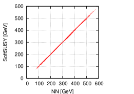
(f) $m_{s\mu}^{L}$

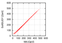
(g) $m_{s\tau}^{1}$

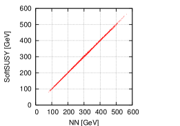
(h) $m_{s\tau}^{2}$

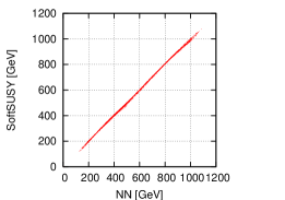
(i) $m_{sd}^{R}$

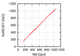
(j) $m_{sd}^{L}$

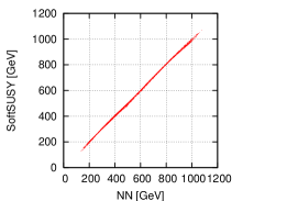
(k) $m_{su}^{R}$

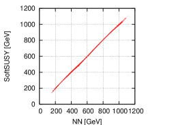
(l) $m_{su}^{R}$

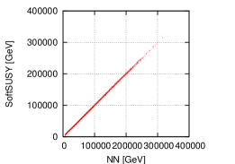
(m) $m_{s\tau}(1,1)$

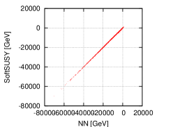
(n) $m_{s\tau}(1,3)$

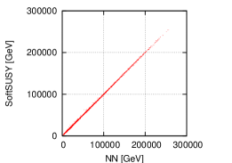
(o) $m_{s\tau}(2,2)$

Figure 2: Correlation plots comparing the mass spectrum [GeV] output of SoftSUSY with the neural network approximations NN. Subfigures (m)-(o) show the components of the mass matrix defining $m_{s\tau}^{1,2}$.

The training data was produced by uniformly sampling roughly 4000 points within the region of parameter space defined by Table 1. Note that the region of parameter space has been restricted to the vicinity of a SUSY benchmark point considered in Section 4. A simple pre-processing step was used to speed up the network optimization: this involves mapping all inputs and outputs linearly so they have zero mean and a variance of one-half. While MemSys provides algorithms for optimising the network architecture, for our function approximation use-case we found empirically that 10 hidden nodes provided a sufficiently accurate and computationally efficient network architecture.

Figure 2 show correlation plots of the SoftSusy outputs with their neural network equivalents. Figures (a) - (l) illustrate the main mass spectrum components and all but $m_{s\tau}^{1}$ (g) demonstrated excellent correlation coefficients of $>$ 0.9999. The training problems for $m_{s\tau}^{1}$ (g), where the best correlation coefficient achieved was no greater than 0.998, was overcome by breaking the problem up into more basic components. In this case we noted that $m_{s\tau}^{1}$ and $m_{s\tau}^{2}$ are eigenvalues of a (symmetric) $2\times 2$ matrix. By asking the network instead to interpolate over the 3 distinct matrix elements (shown in figures (m) -(o)) and then perform the eigenvalue decomposition independently, it was possible to improve the final correlation on $m_{s\tau}^{1}$ to 0.9999.

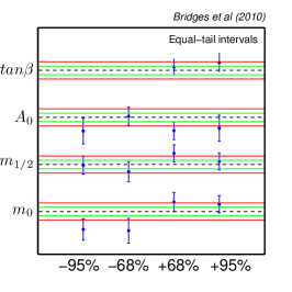
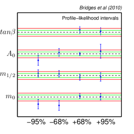
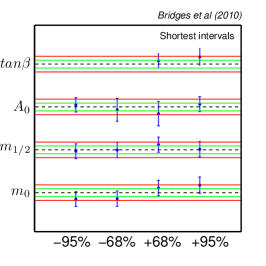
Figure 3: Evaluation of network noise. Horizontal red (green) lines denote error bands for the upper and lower boundaries of 68% (95%) intervals for the CMSSM parameters. The red (green) lines denote $\pm 1\sigma$ ($\pm 2\sigma$) from 100 runs of the SuperBayes fitting package with SoftSusy and quantify numerical/sampling noise. Units of the vertical axis have been rescaled appropriately for display purposes, so that all error bands have the same width. The blue error bars are the corresponding $2\sigma$ error bars based on $10^{4}$ runs using the neural network in place of SoftSusy (with the corresponding rescaling).

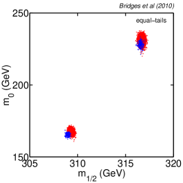
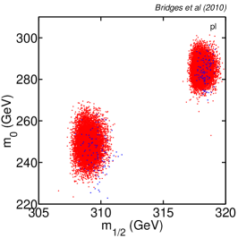
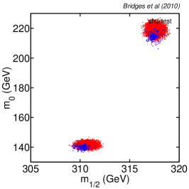
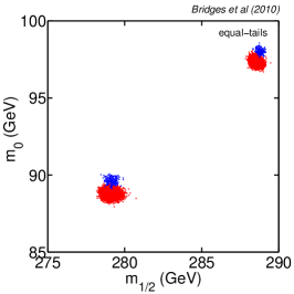
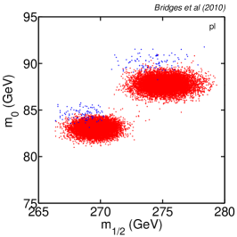
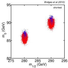
Figure 4: Evaluation of network noise. In the upper (lower) row, red dots give the location of the upper (lower) 68% and 95% intervals for $10^{4}$ runs using the neural network, while blue dots are the locations from 100 runs of the SuperBayes fitting package with SoftSusy.

The impact of replacing SoftSusy with the network is summarized in Fig. 3 and 4. While the approximate mapping will slightly modify the obtained posterior distributions (network noise), this must be compared to the intrinsic variability (sampling noise) in the results due to the finite sampling of techniques such as MCMC and MultiNest. Figure 3 shows that the boundaries of univariate intervals from the two approaches tend to be compatible within about $2\sigma$ of the sampling noise. Figure 4 shows two-dimensional scatter plots of these boundaries. Figure 5 compares the posterior obtained for a single run using the trained network with the posterior obtained with a run using SoftSusy, showing the excellent agreement between the two.

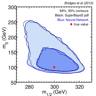
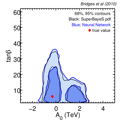
Figure 5: Comparison of Bayesian posteriors between runs of SuperBayes with SoftSusy (black lines, giving 68% and 95% regions) and neural networks (blue lines and corresponding filled regions) obtained using MultiNest, for a typical reconstruction. The agreement between the two methods is excellent, within numerical noise. The red diamond gives the true value for the benchmark point adopted.

The neural network has been trained to perform to high accuracy only in the limited parameter range given in Table 1, since this was sufficient for the specific benchmark point being considered here. If one wanted to consider other regions of the CMSSM parameter space (e.g., the focus point), one would have to extend the network training to include such regions. While we have not experimented with this, based on our experience we believe that this should be straightforward to do.

3.2 A classification network for unphysical parameter values

A very high proportion of points sampled from within the full parameter range are rejected by SoftSusy as unphysical. Furthermore there is no trivial way to identify such points when sampling without resorting to computationally expensive calculations. This is demonstrated by the large degree of overlap seen in Figure 1 between physical (upper points, green) and unphysical (lower points, red) samples in the $m_{0},m_{1/2}$ plane. Such unphysical samples have no valid mass spectrum and so will lie outside of the trained region of the function approximation networks described in the previous section. Thus, we require a means to exclude these points while sampling. Neural networks can be trained to perform for classification such as this, with modification of the training objective function. In this section we will describe classification networks and how they have been implemented for this application.

The aim of classification is to place members of a set into subsets based on inherent properties or features of the individuals, given some pre-classified training data. Formally, classification can be summarised as finding a classifier $\mathcal{C}:\Theta\rightarrow C$ which maps an object from some (typically multi-dimensional) feature space $\Theta$ to its classification label $C$, which is typically taken as one of $\left\{1,...,N\right\}$ where $N$ is the number of distinct classes. Thus the problem of classification is to partition feature space into regions, assigning each region a label corresponding to the appropriate classification. In our context, the aim is to classify points in the parameter space $\Theta$ into one of two classes, physical or unphysical (hence $N=2$), given a set of training data $\mathcal{D}=(\Theta^{(k)},t^{(k)})$, where $t^{(k)}$ is a vector of dimension $N$ that encodes the class label by placing unity in the $C^{\rm th}$ component and zero elsewhere.

In building a classifier using a neural network, it is convenient to view the problem probabilistically. To this end we again consider a 3-layer MLP consisting of an input layer ($\Theta_{l}$), a hidden layer ($h_{j}$), and an output layer ($u_{i}$). In classification networks, however, the outputs are transformed according to the softmax procedure

$$u^{\prime}_{i}=\frac{e^{u_{i}}}{\sum_{i}e^{u_{i}}},$$ (9)

such that they are all non-negative and sum to unity. In this way $u^{\prime}_{i}$ can be interpreted as the probability that the input feature vector $\Theta$ belongs to the $i$th class. A suitable objective function for the classification problem is then

$$\mathcal{L}(\mathbf{b})=\sum_{k}\sum_{i}t^{(k)}_{i}\ln u^{\prime}_{i}(\Theta^{(k)},\mathbf{b}),$$ (10)

where $k$ is an index over the training dataset and $i$ is an index over the $N$ classes. One then wishes to choose network parameters $\mathbf{b}$ so as to maximise this objective function as the training progresses. Training of this network was again performed using the MemSys package as previously described. In our context, the network has just two (transformed) outputs $u^{\prime}_{1}$ and $u^{\prime}_{2}$, which give the probabilities that the input $\Theta$ is physical or unphysical. We partition $\Theta$ space, albeit with some loss of information, by labeling regions according to whether $u^{\prime}_{1}$ or $u^{\prime}_{2}$ exceeds some threshold value.

The training data was taken as a set of uniform samples of roughly 30,000 prior samples equally divided between physical and unphysical status. Again a pre-processing step was carried out so that all inputs were re-mapped to have zero mean and variance of one-half to improve training efficiency. The number of hidden nodes was selected manually and nine hidden nodes were found to perform well.

It is common in signal processing to graphically represent the efficiency of a classifier using a receiver operating characteristic (ROC) curve which plots the true positive rate (TPR) versus the false positive rate (FPR) for increments of the classifiers discrimination threshold. In this case the network outputs $u^{\prime}_{i}$ can be considered probabilities and so one can set a probability threshold above which the classifier should record a positive detection of membership. Variation of this criterion allows classifiers to make a tradeoff between the FPR and the TPR. The left panel of figure 6 shows the ROC curve for the network classifier (solid line). An ideal classifier produces a step-function ROC curve with a TPR of 1 for all values of the threshold whereas a random classifier (black line) always provides equal numbers of true and false positives. For this analysis, adequate results were obtained using a threshold of 0.5, which produces a TPR of $99.8\%$ and a FPR of less than $10\%$. It is possible to obtain arbitrarily small FPR by reducing the threshold (as shown in the right panel of figure 6), however this does result in smaller values of the TPR. Figure 7 demonstrates however that the precise choice of threshold has a minimal effect on the final posteriors obtained.

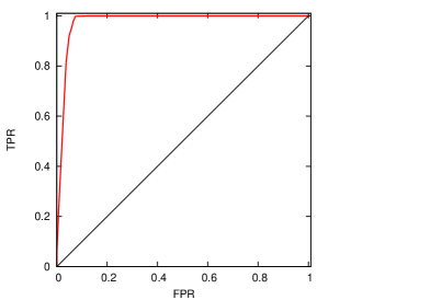
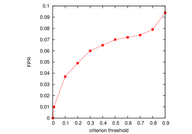
Figure 6: Left panel: Receiver Operating Characteristic (ROC) curve of the neural network classifier for physical and unphysical regions of parameter space (red curve) and a random classifier (black curve). Right panel: False Positive Rate (FPR) as a function of criterion threshold.

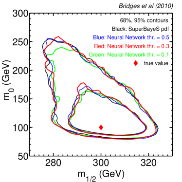
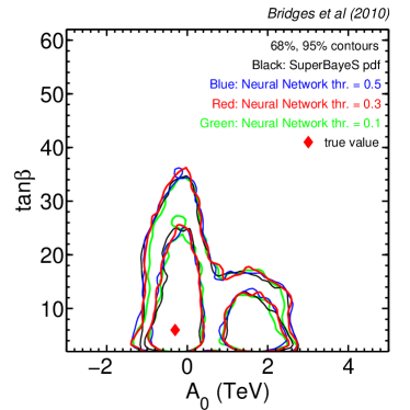
Figure 7: Comparison of Bayesian posteriors between runs of SuperBayes with SoftSusy (black contours, giving 68% and 95% regions) and neural networks for different values of the classification threshold adopted (coloured contours, threshold value according to the legend). The agreement between all posteriors (within numerical noise) demonstrates the classifier’s resiliance to changes in the threshold value.

4 Coverage of intervals at the ATLAS benchmark

Recently the ATLAS collaboration has studied, the so-called “SU3” benchmark point, which is found in the bulk region, assuming an integrated luminosity of 1 $\rm fb^{-1}$ [54]. The analysis considered dilepton and lepton+jets final states from the decay chain ${\widetilde{q}}_{L}\rightarrow\chi^{0}_{2}(\rightarrow\widetilde{l}^{\pm}l^{\mp})q\rightarrow\chi^{0}_{1}l^{+}l^{-}q$ and high-$p_{T}$ and large missing transverse energy from the decay chain ${\widetilde{q}}_{R}\rightarrow\chi^{0}_{1}q$. The aim was to reconstruct the CMSSM (mSUGRA in the ATLAS analysis) model parameters evaluating the accuracy in the reconstruction. For this they have done a MCMC exploration. In a recent work some of us have investigated the analogous constraints using the MultiNest algorithm and the profile likelihood ratio with and without constraints from dark matter relic abundance [34].

	$m_{\chi_{1}^{0}}$	$m_{\chi_{2}^{0}}-m_{\chi_{1}^{0}}$	$m_{\widetilde{q}}-m_{\chi_{1}^{0}}$	$m_{\widetilde{l}}-m_{\chi_{1}^{0}}$
$m_{\chi_{1}^{0}}$	$3.27$	$-12.7$	$-4.89$	$-10.04$
$m_{\chi_{2}^{0}}-m_{\chi_{1}^{0}}$		$476$	$4.23$	$128$
$m_{\widetilde{q}}-m_{\chi_{1}^{0}}$			$8.87$	$8.50$
$m_{\widetilde{l}}-m_{\chi_{1}^{0}}$				$132$

Table 2: Fisher matrix for the ATLAS likelihood employed in the analysis. All entries have been multiplied by $10^{3}$ and are in units of GeV^-2.

Table 2 shows the inverse of the covariance matrix (i.e., the Fisher matrix) for sparticle masses used in this study, which is based on the parabolic approximation of the log-likelihood function reported in Ref. [54]. This likelihood function is based on the measurement of edges and thresholds in the invariant mass distributions for various combinations of leptons and jets in final state of the selected candidate SUSY events. Note that the relationship between the sparticle masses and the directly observable mass edges is highly non-linear, so a Gaussian is likely to be a poor approximation to the actual likelihood function. Furthermore, these edges share several sources of systematic uncertainties, such as jet and lepton energy scale uncertainties, which are only approximately communicated in Ref. [54]. While noting that these approximations to the likelihood function may omit essential information in the data, we proceed to assess the coverage of the intervals in this idealized setting.

In order to assess coverage, we not only need the likelihood function ($P(d|\Theta)$ with $d$ fixed), but we also need the ability to generate pseudo-experiments with $\Theta$ fixed. Here we introduce an additional simplification that $P(d|\Theta)$ is also a multivariate Gaussian with the same covariance structure. For a multivariate Gaussian, one would expect the profile likelihood to have nearly perfect coverage properties, unless there is a breakdown in one of the regularity requirements present in Wilks’s theorem  [55]. Two of the requirements that are most likely to be violated (or lead to a slow convergence to the asymptotic properties assured by Wilks’s theorem) are related to the presence of boundaries on the parameter space or parameters that have no impact on the likelihood function in certain regions of the parameter space. As discussed above, excluding unphysical regions from the CMSSM parameter space imposes complicated boundary conditions. Similarly, in some regions of parameter space, certain interactions can be highly suppressed (either due to quantum effects or phase space considerations), in which case some parameters may have little effect on the likelihood function. In the case of four CMSSM parameters and four non-degenerate measurements, the latter is not an issue, but boundary effects may be relevant.

In addition to the complications due to the structure of the model itself, there are other issues which could spoil the expected coverage properties. First, some algorithmic artifact or shortcoming associated with the procedure that creates the intervals. These are complex, high dimensional problems, so it is possible that the algorithms may not perform in practice as well as they should in principle. Secondly, if the likelihood function is not strong enough to overcome the prior and they prefer different regions of parameter space, one may expect poor coverage properties.

The sensitivity to priors and comparisons with the profile likelihood ratio were considered for the same ATLAS benchmark point in Ref. [34]; reasonable agreement between the different approaches was found, indicating the likelihood function is dominating the inference. Thus, we focus our attention on effects from algorithmic artifacts and the complicated boundaries of the physical CMSSM.

In order to isolate algorithmic effects, we begin by constructing intervals in the weak scale masses $m$ (as opposed to the more fundamental CMSSM parameters $\theta$). The likelihood function is invariant under these reparametrizations, and it is trivial to extend the domain of the weak scale masses so that boundary effects are absent. In total $10^{4}$ pseudo-experiments were analyzed using MCMC using $10^{6}$ samples each. A flat prior was used on the space of $m$. From the MCMC samples, equal-tail and shortest credible intervals were constructed by marginalizing the posterior distribution to each of the four parameters. Additionally, profile likelihood intervals were constructed by maximizing the likelihood across the samples. Figure 8 shows that each of the restricted 1-d intervals covers with the stated rate for each of the methods. Thus, we conclude that our MCMC algorithm is performing as expected for this likelihood function.

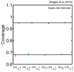
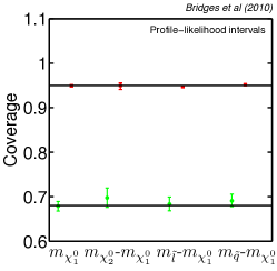
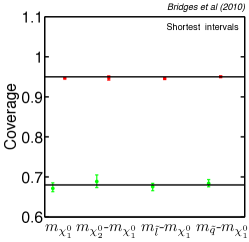
Figure 8: Test of coverage for a toy 8D MCMC model. Green (red) is for the nominal 68% (95%) error. The recovered coverage is compatible with the exact value within the errors due to numerical/sampling noise. Error bars denote the standard deviation from $10^{4}$ reconstructions with MCMC.

To assess the coverage in the restricted space of the physically realizable CMSSM requires several additional ingredients. First, we must introduce the mapping $\Theta\to{\mbox{\boldmath$m$}}$ and the boundaries on $\Theta$ corresponding to physically realizable parameter points. It is not computationally feasible to use SoftSusy for so many repeated likelihood evaluations, thus we rely on the neural network approximation to the mapping and a second network for classification of the physical points. Additionally, we must specify a prior on the space of $\Theta$; for this we used log priors in $m_{0},m_{1/2}$ and note there was little sensitivity to this choice in previous studies based on the same ATLAS likelihood function [34]. We construct $10^{4}$ pseudo-experiments and analyze them with both MCMC (using a Metropolis-Hastings algorithm) and MultiNest. Each realization is run as an independent chain until we gather a total of $10^{6}$ posterior samples in the MCMC chain. For MultiNest, we run until the tolerance criterium is satisfied (with a tolerance parameter 0.5), which results in about 50k posterior samples. Altogether, our neural network MCMC runs have performed a total of $4\times 10^{10}$ likelihood evaluations, in a total computational effort of approximately $2\times 10^{4}$ CPU-minutes. We estimate that the same computation using SoftSusy would have taken about 1100-CPU years, which is at the boundary of what is feasible today, even with a massive parallel computing effort. By using the neural network, we observe a speed-up factor of about $3\times 10^{4}$ compared with scans using the explicit spectrum calculator.

As above, the posterior samples were used to form equal-tailed, central, and profile-likelihood based intervals for each of the four fundamental CMSSM parameters. Coverage was then computed for each type of interval. In order to quantify the uncertainty in the coverage introduced by sampling noise (i.e., the finite length of our MCMC chains) and by the neural network approximation to the full RGE calculation, we proceeded as follows. First, for each lower/upper limit (at a given confidence level) we built the quantity $\sigma_{\text{tot}}=(\sigma^{2}_{\text{SN}}+\sigma^{2}_{\text{NN}})^{1/2}$, where $\sigma_{\text{SN}}$ is the sampling noise standard deviation while $\sigma_{\text{NN}}$ is the standard deviation from the neural network noise for that limit, both of which have been estimated by the pseudo-experiments of section 3.1. We then shifted the intervals uniformly downwards or upwards (keeping the intervals’ length constant) by an amount given by the appropriate $\sigma_{\text{tot}}$. This leads to a higher/lower coverage (depending on the direction of the shift and the limit being considered), which we used as an estimation of the standard deviation of the coverage value itself. This quantity is shown as an errorbar on the coverage values. We note that because of the large number of pseudo-experiments employed, the statistical noise from the binomial process itself is negligible compared with the above uncertainties. For the 2-d intervals we proceeded in a similar fashion, with the direction of the shift (in the 2-d plane) chosen to be parallel to the line connecting the mean value of the 2-d upper/lower limit (i.e., this is the most conservative choice for the error).

The results are shown in Fig. 9, where it can be seen that the methods have substantial over-coverage (are conservative). The coverage of 2-d intervals is also shown in Fig. 10.

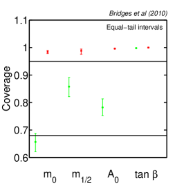
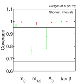
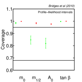
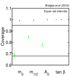
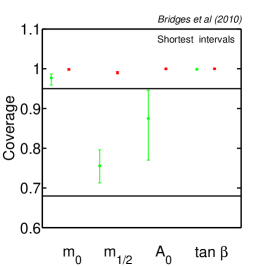
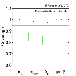
Figure 9: Coverage for various types of intervals for the CMSSM parameters, from $10^{4}$ realizations. The top row employs MCMC for the reconstruction (each pseudo-experiment is reconstructed with $10^{6}$ samples), while to bottom row uses MultiNest (with $5\times 10^{4}$ samples per pseudo-experiment). Green (red) is for the 68% (95%) error.

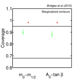
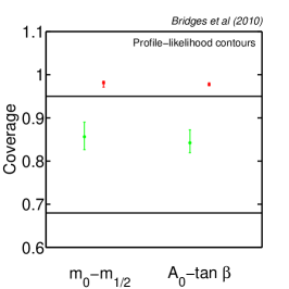
Figure 10: Coverage for various types of two-dimensional intervals for the CMSSM parameters, from $10^{4}$ realizations based on MCMC (with $10^{6}$ samples per pseudo-experiment). Green (red) is for the 68% (95%) error.

4.1 Discussion of coverage results

While it is difficult to unambiguously attribute the over-coverage to a specific cause, the most likely cause is the effect of boundary conditions imposed by the CMSSM. An example of such boundaries and how they compare with the extent of the likelihood function is shown in Fig. 11. This figure shows regions in some of the weak-scale mass combinations entering the likelihood which can be realized within the CMSSM (green shades). The red ellipses are $1\sigma$ contours from the likelihood, and are centered around the benchmark value. It is clear that likelihood extends beyond the boundaries imposed by the CMSSM, which leads to a slow convergence of the profile likelihood ratio to the asymptotic chi-square distribution.

Recall that the profile likelihood ratio is defined as $\lambda(\theta)=L(\theta,\hat{\hat{\psi}})/L(\hat{\theta},\hat{{\psi}})$, where $\hat{\hat{\psi}}$ is the conditional maximum likelihood estimate (MLE) of $\psi$ with $\theta$ fixed, and $\hat{\theta}$, $\hat{\psi}$ are the unconditional MLEs. When the fit is performed in the space of the weak-scale masses, there are no boundary effects, and the distribution of $-2\ln\lambda({\mbox{\boldmath$m$}})$ (when $m$ is true) is distributed as a chi-square with a number of degrees of freedom given by the dimensionality of $m$. Since the likelihood is invariant under reparametrizations, we expect $-2\ln\lambda(\theta)$ to also be distributed as a chi-square. If the boundary is such that ${\mbox{\boldmath$m$}}(\hat{\theta},\hat{\psi})\neq\hat{{\mbox{\boldmath$m$}}}$ or ${\mbox{\boldmath$m$}}(\theta,\hat{\hat{\psi}})\neq\hat{\hat{{\mbox{\boldmath$m$}}}}$, then the resulting interval will modified. More importantly, one expects the denominator $L(\hat{\theta},\hat{\psi})<L(\hat{{\mbox{\boldmath$m$}}})$ since $m$ is unconstrained, which will lead to $-2\ln\lambda(\theta)<-2\ln\lambda({\mbox{\boldmath$m$}})$. In turn, this means more parameter points being included in any given contour, which leads to over-coverage. Evidence for this effect can be seen in Fig. 12, which shows the value of $-2\ln\lambda$ for the scans in $m$ and $\Theta$.

The impact of the boundary on the distribution of the profile likelihood ratio is not insurmountable. It is not fundamentally different than several common examples in high-energy physics where an unconstrained MLE would like outside of the physical parameter space. Examples include downward fluctuations in event-counting experiments when the signal rate is bounded to be non-negative. Another common example is the measurement of sines and cosines of mixing angles that are physically bounded between $[-1,1]$, though an unphysical MLE may lie outside this region. The size of this effect is related to the probability that the MLE is pushed to a physical boundary. If this probability can be estimated, it is possible to estimate a corrected threshold on $-2\ln\lambda$. For a precise threshold with guaranteed coverage, one must resort to a fully frequentist Neyman Construction.

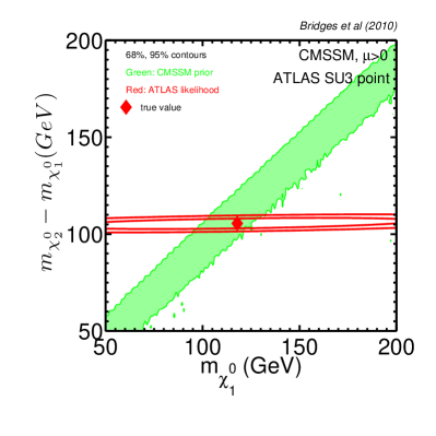
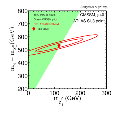
Figure 11: Illustration of the boundary effects coming from the physically realizable CMSSM (green region) with respect to the unconstrained likelihood expressed in the weak-scale masses (red ellipses). The likelihood extends beyond the boundaries imposed by the CMSSM, which leads to a slow convergence of the profile likelihood ratio to the asymptotic chi-square distribution.

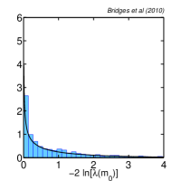
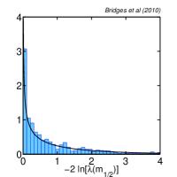
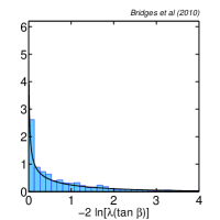
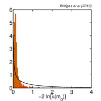
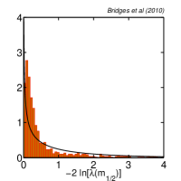
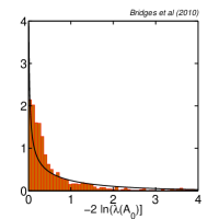
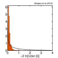
Figure 12: The distribution of $-2\ln\lambda$ for the scans in $m$ (top row) and $\Theta$ (bottom row) from repeated realizations of pseudo-experiments. The solid line is a $\chi^{2}$ distribution with 1 dof expected from Wilks’ theorem. The distributions from scans in the weak-scale masses (top row) follow quite closely the $\chi^{2}$ distribution, while this is not the case for the scans using the CMSSM parameters as fundamental quantities.

5 Summary and conclusions

We have presented a coverage study of state of the art techniques used for supersymmetric parameter estimation based on realistic toy data from an ATLAS sensitivity study. The techniques employ both MCMC and nested sampling to explore the parameter space and the posterior samples can be used to provide both Bayesian credible intervals and profile likelihood-based frequentist confidence intervals. We have tested our coverage analysis pipeline in a simple Gaussian toy model with the same dimensionality as the supersymmetric parameter space under consideration, and have confirmed the reliability of both the Bayesian posterior and profile likelihood intervals in this setting obtained with nested sampling and MCMC.

The likelihood function used in these studies is a simplified representation of the actual likelihood based on the information in the ATLAS publication. We note that in order to perform coverage studies, one not only needs the ability to evaluate the likelihood function based on the pseudo-experiment, but also the ability to generate the pseudo-experiment itself. Both the representation of the likelihood function and the ability to generate pseudo-experiment are now possible with the workspace technology in RooFit/RooStats [57]. We encourage future experiments to publish their likelihoods using this technology. Furthermore, we point out that these likelihood functions should include the nuisance parameters associated with experimental systematics, since they may be correlated across the different measurements entering a global fit.

We observe good coverage properties for intervals based directly on the weak-scale sparticle masses, confirming the reliability of both the Bayesian credible intervals and profile likelihood intervals obtained with nested sampling and MCMC in this setting. In contrast, we observe significant over-coverage in the fundamental CMSSM parameters, which we attribute to boundaries in the parameter space imposed by requirements of physically realizable theories. Our findings are specific to the benchmark point considered in our analysis, and coverage properties of benchmark points in different regions of the CMSSM parameter space might differ substantially. Currently, there is no known way to generalize the results, thus coverage requires a case-by-case analysis. The technique presented in this paper is, however, readily applicable to any benchmark point, provided a suitable likelihood function for LHC data is available, and that the neural network training is extended appropriately.

Coverage studies are computationally expensive to perform, and the most intensive step for an individual likelihood evaluation in this context is the evaluation of the RGEs in the spectrum calculators. Thus, we have introduced a method to approximate the spectrum calculators with neural networks. We observe consistency in the obtained intervals with speed-ups of $10^{4}$ by utilizing neural network approximations. In principle, the same techniques can be applied to accelerate the computation of other observables, such as the relic density.

In order to assess the actual coverage properties of both Frequentist and Bayesian intervals obtained from future data, it will be unavoidable to perform detailed studies using a large number of pseudo-experiments. This paper demonstrated for the first time how neural network techniques can be employed to achieve a very significant speed-up with respect to conventional spectrum calculators. Such methods are necessary in order to cope with the very large number of likelihood evaluations required in coverage studies. Our work is but a first step towards making accelerated inference techniques more widespread and more easily accessible to the community.

Acknowledgements

The authors wish to thank Louis Lyons for many useful discussions and suggestions, the authors of Ref [56] for discussing their work with us prior to publication, Yashar Akrami, Jan Conrad and Pat Scott for helpful comments on a draft of this work and an anonymous referee for useful comments. We would like to thank the PROSPECTS workshop (Stockholm, Sept 2010) organizers, the BIRS Discovery Challenges workshop 2010 (Banff, July 2010) organizers and the CosmoStats09 conference (Ascona, July 2009) organizers for stimulating meetings which offered the opportunity to discuss several of the issues presented in this paper. K.C. is supported by the US National Science Foundation grants PHY-0854724 and PHY-0955626. F.F. is supported by Trinity Hall, Cambridge. R.RDA is supported by the project PROMETEO (PROMETEO/2008/069) of the Generalitat Valenciana and the Spanish MICINN’s Consolider-Ingenio 2010 Programme under the grant MULTIDARK CSD2209-00064. R.T. would like to thank the Galileo Galilei Institute for Theoretical Physics for hospitality and the INFN and the EU FP6 Marie Curie Research and Training Network “UniverseNet” (MRTN-CT-2006-035863) for partial support. The use of Imperial College London High Performance Computing service is gratefully acknowledged. Part of this work was performed using the Darwin Supercomputer of the University of Cambridge High Performance Computing Service (http://www.hpc.cam.ac.uk/), provided by Dell Inc. using Strategic Research Infrastructure Funding from the Higher Education Funding Council for England.

References

- [1] G. L. Kane, C. Kolda, L. Roszkowski, and J. D. Wells, Study of constrained minimal supersymmetry, Phys. Rev. D 49 (June, 1994) 6173–6210, [arXiv:hep-ph/9312272].
- [2] A. Brignole, L. E. Ibáñez, and C. Muñoz, Soft Supersymmetry-Breaking Terms from Supergravity and Superstring Models, in Perspectives on Supersymmetry (G. L. Kane, ed.), p. 125, 1998. arXiv:hep-ph/9707209.
- [3] M. Drees and M. M. Nojiri, Neutralino relic density in minimal N=1 supergravity, Phys. Rev. D 47 (Jan., 1993) 376–408, [arXiv:hep-ph/9207234].
- [4] H. Baer and M. Brhlik, Cosmological relic density from minimal supergravity with implications for collider physics, Phys. Rev. D 53 (Jan., 1996) 597–605, [arXiv:hep-ph/9508321].
- [5] J. Ellis, T. Falk, K. A. Olive, and M. Srednicki, Calculations of neutralino-stau coannihilation channels and the cosmologically relevant region of MSSM parameter space, Astroparticle Physics 13 (May, 2000) 181–213, [arXiv:hep-ph/9905481].
- [6] J. Ellis, T. Falk, G. Ganis, K. A. Olive, and M. Srednicki, The CMSSM parameter space at large /tan, Physics Letters B 510 (June, 2001) 236–246, [arXiv:hep-ph/0102098].
- [7] L. Roszkowski, R. Ruiz de Austri, and T. Nihei, New cosmological and experimental constraints on the CMSSM, Journal of High Energy Physics 8 (Aug., 2001) 24, [arXiv:hep-ph/0106334].
- [8] A. B. Lahanas and V. C. Spanos, Implications of the pseudo-scalar Higgs boson in determining the neutralino dark matter, European Physical Journal C 23 (Mar., 2002) 185–190, [arXiv:hep-ph/0106345].
- [9] E. A. Baltz and P. Gondolo, Markov chain Monte Carlo exploration of minimal supergravity with implications for dark matter, JHEP 10 (2004) 052, [hep-ph/0407039].
- [10] B. C. Allanach and C. G. Lester, Multi-Dimensional mSUGRA Likelihood Maps, Phys. Rev. D73 (2006) 015013, [hep-ph/0507283].
- [11] B. C. Allanach, Naturalness priors and fits to the constrained minimal supersymmetric standard model, Phys. Lett. B635 (2006) 123–130, [hep-ph/0601089].
- [12] R. Ruiz de Austri, R. Trotta, and L. Roszkowski, A Markov chain Monte Carlo analysis of the CMSSM, JHEP 05 (2006) 002, [hep-ph/0602028].
- [13] B. C. Allanach, C. G. Lester, and A. M. Weber, The Dark Side of mSUGRA, JHEP 12 (2006) 065, [hep-ph/0609295].
- [14] L. Roszkowski, R. R. de Austri, and R. Trotta, On the detectability of the CMSSM light Higgs boson at the Tevatron, JHEP 04 (2007) 084, [hep-ph/0611173].
- [15] B. C. Allanach, K. Cranmer, C. G. Lester, and A. M. Weber, Natural priors, CMSSM fits and LHC weather forecasts, JHEP 0708 (2007) 023, [0705.0487].
- [16] L. Roszkowski, R. Ruiz de Austri, and R. Trotta, Implications for the Constrained MSSM from a new prediction for , JHEP 07 (2007) 075, [0705.2012].
- [17] L. Roszkowski, R. R. de Austri, J. Silk, and R. Trotta, On prospects for dark matter indirect detection in the Constrained MSSM, Phys. Lett. B671 (2009) 10–14, [0707.0622].
- [18] B. C. Allanach, M. J. Dolan, and A. M. Weber, Global Fits of the Large Volume String Scenario to WMAP5 and Other Indirect Constraints Using Markov Chain Monte Carlo, JHEP 08 (2008) 105, [0806.1184].
- [19] B. C. Allanach and D. Hooper, Panglossian Prospects for Detecting Neutralino Dark Matter in Light of Natural Priors, JHEP 10 (2008) 071, [0806.1923].
- [20] G. D. Martinez, J. S. Bullock, M. Kaplinghat, L. E. Strigari, and R. Trotta, Indirect Dark Matter Detection from Dwarf Satellites: Joint Expectations from Astrophysics and Supersymmetry, JCAP 0906 (2009) 014, [0902.4715].
- [21] F. Feroz and M. P. Hobson, Multimodal nested sampling: an efficient and robust alternative to MCMC methods for astronomical data analysis, Mon. Not. Roy. Astron. Soc. 384 (2008) 449–463, [0704.3704].
- [22] F. Feroz, M. P. Hobson, and M. Bridges, MultiNest: an efficient and robust Bayesian inference tool for cosmology and particle physics, Mon. Not. Roy. Astron. Soc. 398 (2009) 1601–1614, [0809.3437].
- [23] R. Trotta, F. Feroz, M. Hobson, L. Roszkowski, and R. Ruiz de Austri, The impact of priors and observables on parameter inferences in the constrained MSSM, Journal of High Energy Physics 12 (Dec., 2008) 24, [0809.3792].
- [24] J. Skilling, Nested Sampling for Bayesian Computations, Proc. Valencia/ISBA World Meeting on Bayesian Statistics (2006).
- [25] F. Feroz et al., Bayesian Selection of sign(mu) within mSUGRA in Global Fits Including WMAP5 Results, JHEP 10 (2008) 064, [0807.4512].
- [26] F. Feroz, M. P. Hobson, L. Roszkowski, R. Ruiz de Austri, and R. Trotta, Are BR() and consistent within the Constrained MSSM?, 0903.2487.
- [27] S. S. AbdusSalam, B. C. Allanach, F. Quevedo, F. Feroz, and M. Hobson, Fitting the Phenomenological MSSM, Phys. Rev. D81 (2010) 095012, [0904.2548].
- [28] R. Trotta, R. R. de Austri, and C. P. d. l. Heros, Prospects for dark matter detection with IceCube in the context of the CMSSM, JCAP 0908 (2009) 034, [0906.0366].
- [29] S. S. AbdusSalam, B. C. Allanach, M. J. Dolan, F. Feroz, and M. P. Hobson, Selecting a Model of Supersymmetry Breaking Mediation, Phys. Rev. D80 (2009) 035017, [0906.0957].
- [30] M. E. Cabrera, J. A. Casas, and R. Ruiz d Austri, MSSM Forecast for the LHC, JHEP 05 (2010) 043, [0911.4686].
- [31] G. Bertone, D. G. Cerdeno, M. Fornasa, R. R. de Austri, and R. Trotta, Identification of Dark Matter particles with LHC and direct detection data, Phys. Rev. D82 (2010) 055008, [1005.4280].
- [32] P. Scott et al., Direct Constraints on Minimal Supersymmetry from Fermi-LAT Observations of the Dwarf Galaxy Segue 1, JCAP 1001 (2010) 031, [0909.3300].
- [33] D. E. Lopez-Fogliani, L. Roszkowski, R. R. de Austri, and T. A. Varley, A Bayesian Analysis of the Constrained NMSSM, Phys. Rev. D80 (2009) 095013, [0906.4911].
- [34] L. Roszkowski, R. Ruiz de Austri, and R. Trotta, Efficient reconstruction of constrained MSSM parameters from LHC data: A case study, Phys. Rev. D 82 (Sept., 2010) 055003, [0907.0594].
- [35] R. Lafaye, T. Plehn, M. Rauch, and D. Zerwas, Measuring supersymmetry, European Physical Journal C 54 (Apr., 2008) 617–644, [0709.3985].
- [36] Y. Akrami, P. Scott, J. Edsjo, J. Conrad, and L. Bergstrom, A Profile Likelihood Analysis of the Constrained MSSM with Genetic Algorithms, JHEP 04 (2010) 057, [0910.3950].
- [37] S. M. Moore and C. Leger, Some aspects of matching priors, in Mathematical statistics and applications: Festschrift for Constance van Eeden (Beachwood, OH: Institute of Mathematical Statistics), pp. 31–43. http://projecteuclid.org/ euclid.lnms/1215091929, 2003.
- [38] H. P. L. Lyons and A. de Roeck, Some aspects of matching priors, in Proceedings of the PHYSTAT LHC Workshop on Statistical Issues for LHC Physics (CERN, Geneva, 27-29 June 2007). CERN Yellow Report 2008-001, 2008.
- [39] T. Auld, M. Bridges, M. P. Hobson, and S. F. Gull, Fast cosmological parameter estimation using neural networks, Mon. Not. Roy. Astron. Soc. Lett. 376 (2007) L11–L15, [astro-ph/0608174].
- [40] R. Trotta, Bayes in the sky: Bayesian inference and model selection in cosmology, Contemp. Phys. 49 (2008) 71–104, [0803.4089].
- [41] B. C. Allanach, S. Kraml, and W. Porod, Theoretical uncertainties in sparticle mass predictions from computational tools, JHEP 03 (2003) 016, [hep-ph/0302102].
- [42] B. C. Allanach, SOFTSUSY: A program for calculating supersymmetric spectra, Computer Physics Communications 143 (Mar., 2002) 305–331, [arXiv:hep-ph/0104145].
- [43] G. H. D.E. Rumelhart and R. Williams, Learning representations by backpropagating errors., Nature 323 (1986) 533–536.
- [44] J. C. Mason and M. G. Cox, Radial basis functions for multivariate interpolation: a review, in In Algorithms for Approximation, pp. 143–167. Clarendon Press, 1987.
- [45] V. Vapnik, The Nature of Statistical Learning Theory. Springer, New York, 1995.
- [46] R. O. L. Breiman, J.H. Friedman and C. Stone, Classification and Regression Trees. Wadsworth, Belmont California, 1983.
- [47] J. Friedman, Greedy function approximation: A gradient boosting machine., Ann. Statist. 29 (2001) 1189–1232.
- [48] G. Cybenko, Approximations by superpositions of sigmoidal functions., Mathematics of Control, Signals, and Systems 4 (2001) 303–314.
- [49] A. P. M. Leshno, V. Ya Lin and S. Schocken, Multilayer feedforward networks with a nonpolynomial activation function can approximate any function, Neural Netw. 6 (1993) 861.
- [50] A. Bryson and Y. Ho, Applied optimal control: optimization, estimation, and control. Blaisdell Publishing Company, 1969.
- [51] D. MacKay, Bayesian Methods for Adaptive Models. California Institute of Technology, 1992.
- [52] M. P. Hobson and A. N. Lasenby, The entropic prior for distributions with positive and negative values, Mon. Not. R. Astr. Soc. 298 (Aug., 1998) 905–908, [arXiv:astro-ph/9810240].
- [53] S. Gull and J. Skilling, Quantified maximum entropy: MemSys 5 users’ manual. Maximum Entropy Data Consultants Ltd, Royston,U.K., 1999.
- [54] The ATLAS Collaboration: G. Aad, E. Abat, B. Abbott, J. Abdallah, A. A. Abdelalim, A. Abdesselam, O. Abdinov, B. Abi, M. Abolins, H. Abramowicz, and et al., Expected Performance of the ATLAS Experiment - Detector, Trigger and Physics, ArXiv e-prints (Dec., 2009) [0901.0512].
- [55] S. Wilks, The large-sample distribution of the likelihood ratio for testing composite hypotheses, Ann. Math. (1938) 60–62.
- [56] Y. Akrami, C. Savage, P. Scott, J. Conrad, and J. Edsjö, Statistical coverage for supersymmetric parameter estimation: a case study with direct detection of dark matter, Private communication (2010).
- [57] L. Moneta, K. Belasco, K. Cranmer, A. Lazzaro, D. Piparo, et al., The RooStats Project, Proceedings of Science (2010) Proceedings of the 13th International Workshop on Advanced Computing and Analysis Techniques in Physics Research, India, [arXiv:1009.1003].