A Spectroscopic Method to Measure the Superfluid Fraction of an Ultracold Atomic Gas

Abstract

We perform detailed analytical and numerical studies of a recently proposed method for a spectroscopic measurement of the superfluid fraction of an ultracold atomic gas [N. R. Cooper and Z. Hadzibabic, Phys. Rev. Lett. 104, 030401 (2010)]. Previous theoretical work is extended by explicitly including the effects of non-zero temperature and interactions, and assessing the quantitative accuracy of the proposed measurement for a one-component Bose gas. We show that for suitably chosen experimental parameters the method yields an experimentally detectable signal and a sufficiently accurate measurement. This is illustrated by explicitly considering two key examples: First, for a weakly interacting three-dimensional Bose gas it reproduces the expected result that below the critical temperature the superfluid fraction closely follows the condensate fraction. Second, it allows a clear quantitative differentiation of the superfluid and the condensate density in a strongly interacting Bose gas.

I Introduction

Ultracold atomic gases provide a highly controllable experimental setting for studies of many-body quantum phenomena such as Bose-Einstein condensation Anderson1995 and superfluidity ColdgasSF1 ; ColdgasSF2 ; ColdgasSF3 (for a review see RevModPhys2008 ). The physical phenomena studied in these systems are often analogous to those occurring in other many-body systems, in particular solid state materials and liquid helium. Moreover, the flexibility in experimentally designing the geometry and interactions in atomic gases offers the possibility to experimentally access physical regimes which are of theoretical interest but could so far not be observed. At the same time, the experimental probes used in atomic physics are often quite different from those traditionally used in condensed matter experiments and discussed in the theoretical literature. In particular, for atomic gases there is no general experimentally established method allowing a quantitative measurement of the superfluid fraction, which is traditionally defined through the fluid’s response to rotation and the emergence of a non-classical moment of inertia Leggett1999 . In classic experiments on liquid helium Andronikashvili1946 , under rotation of the walls of the container a perfect superfluid remains metastable in the zero angular momentum state as long as the rotation rate does not exceed the critical velocity for a superfluid flow. More generally, the fraction of the fluid which does not rotate with the walls quantitatively defines the superfluid fraction.

Only very recently some ideas on how to measure the superfluid fraction of an ultracold atomic gas have been formulated Riedl2009 ; HoZhou2009 ; CooperHadzibabic2010 . Specifically, in Ref. CooperHadzibabic2010, a spectroscopic method was proposed, which closely follows the traditional definition of the superfluid density but allows a signal readout which plays to the strengths of atomic physics. This proposal builds on the recent developments in the use of optical fields to induce artificial gauge fields for ultracold atoms dalibardreview . The key idea is that if slow rotation of the gas is induced by an optical gauge field, this creates a natural coupling between the external (angular momentum) and the internal (hyperfine) atomic degrees of freedom. Measuring the populations of hyperfine states in an atomic cloud then allows a direct readout of the angular momentum induced by the rotation, and thus a measurement of the moment of inertia and the superfluid fraction.

The basic connection between the hyperfine populations and the superfluid fraction was pointed out in Ref. CooperHadzibabic2010, by considering the difference between a perfect superfluid with no angular momentum and a fully relaxed gas which exhibits the classical value of the moment of inertia. Here we extend this theoretical work in several ways. First, we include in our calculations the effects of non-zero temperature and interactions in the gas, which broaden the distribution of angular momenta around zero for a metastable superfluid, and around the classical value set by the imposed rotation for a fully relaxed gas. This allows us to assess the quantitative accuracy of the proposed measurement, and to estimate the experimental parameters which in practice would allow a good compromise between the theoretical accuracy of the method and the experimentally relevant size of the readout signal. Second, we explicitly calculate the expected experimental signal in two important cases: For a weakly interacting Bose gas we show that the spectroscopically deduced superfluid fraction closely follows the condensate fraction below the critical temperature; this confirms that the proposed method gives the expected result in this well understood limit. On the other hand, in the limit of strong interactions the superfluid and the condensate fraction of the gas can be quite different, as is known from the case of liquid helium Griffin1996 . We show that in this limit the spectroscopic measurement is sufficiently accurate to allow a clear experimental distinction between the two quantities.

The paper is organized as follows. In Section II we lay out the theoretical background on the concept of superfluid density and its connection to hyperfine populations in an atomic cloud rotated with use of optically induced gauge potentials. In Section III we give some more details on a specific implementation of gauge fields in an atomic system. In Section IV we discuss the quantitative theoretical corrections to the mapping between the hyperfine populations and the superfluid fraction. To illustrate the effect of these corrections we first consider a normal gas at non-zero temperature; this already allows us to anticipate suitable experimental parameters which lead to sufficiently small theoretical inaccuracies and sufficiently large experimental signals. In Section V we extend our calculations to interacting gases, at both zero and non-zero temperature. Our results for the expected experimental signals in both weakly and strongly interacting gases are presented in Section VI. Finally, Section VII contains a summary of the paper.

II Superfluid density

The concept of a superfluid density, or superfluid fraction, originates in the two-fluid model for the hydrodynamics of superfluid ⁴He, proposed by Tisza tisza1 ; tisza2 and Landau Landau . The fluid, of total density $\rho$, is assumed to consist of a superfluid component, of density $\rho_{s}$, which has vanishing viscosity and flows without dissipation, and a normal component, of density $\rho_{n}=\rho-\rho_{s}$. Landau proposed Landau how to measure these separate components. He envisaged taking superfluid helium at rest in its container, and slowly rotating the walls at a constant angular velocity $\omega$. The normal component equilibrates and moves along with the rotating walls; however, the superfluid component is unaffected and remains at rest. Since only the normal component moves, the moment of inertia of the fluid is determined by $\rho_{n}$, and its ratio to the expected classical moment of inertia (defined by the total density $\rho$) provides the normal fraction $\rho_{n}/\rho$ and hence the superfluid fraction $1-\rho_{n}/\rho$. Note that it is necessary that the trap is not perfectly rotationally symmetric (i.e. the walls must be rough), so that the normal fluid can relax into the steadily rotating state and come into equilibrium by changing its angular momentum.

This method was implemented for superfluid helium in the classic experiments by Andronikashvili Andronikashvili1946 . In those experiments it was not the container that was rotated, but a stack of disks embedded in the fluid. Still, the disks drag just the normal fluid, so measurements of the moment of inertia of the disks (using a torsional oscillator) allowed a determination of the normal and superfluid fractions.

The non-classical moment of inertia arising from the superfluid component provides the standard definition of the superfluid fraction Leggett1999 . To discuss this theoretically, it is customary to consider the fluid to be contained in a ring-shaped toroidal vessel with a radius $R$ much larger than its transverse dimensions $\Delta R$, cf. Fig. 1.

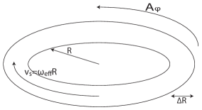
Figure 1: Geometry of the vessel considered in this paper: a torus of radius $R$ with transverse dimensions $\Delta R\ll R$. $A_{\varphi}$ is the gauge potential introduced by light fields, corresponding to rotation with angular frequency $\omega_{\textrm{eff}}$. This induces a superfluid flow with speed $v_{s}$ in the direction opposite to $A_{\varphi}$.

In this case, the classical moment of inertia for $N$ atoms of mass $M$ is given by $I_{\textrm{cl}}=NMR^{2}$. We shall assume this geometry throughout this paper — in part for theoretical simplicity, but also for practical reasons discussed further below. The superfluid fraction is then defined Leggett1999 by the average angular momentum $\langle L\rangle$ picked up under rotation of the vessel with an angular frequency $\omega$:

$$\frac{\rho_{s}}{\rho}\equiv 1-\lim_{\omega\to 0}\left(\frac{\langle L\rangle}{I_{\textrm{cl}}\omega}\right).$$ (1)

The limit $\omega\to 0$ of slow rotation of the vessel is required such that the velocity of the walls of the container, $\omega R$, does not exceed the critical velocity of the superfluid, $\omega R<v_{\rm crit}$. Since finite-size effects can be much more important in ultracold atomic gases than in typical experiments on superfluid helium, it is helpful to expand further on this point. For a very small rotation rate, namely when $\omega<\hbar/2MR^{2}$, even an ideal Bose gas shows a non-classical moment of inertia, and could thus be considered to be superfluid blatt1955 . (For $\omega<\hbar/2MR^{2}$, the lowest-energy single particle state remains the state with vanishing angular momentum, so an ideal condensate has $L=0$.) We define superfluidity in the strongest sense of Ref. blatt1955, , which is the sense that is conventionally applied: the angular momentum is measured with an imposed rotation frequency in the range $\hbar/2MR^{2}<\omega<v_{\rm crit}/R$. The lower limit excludes the ideal Bose gas as a superfluid. For a large system, $R\gg\hbar/Mv_{\rm crit}$, this constitutes a wide range of frequencies. For a weakly interacting Bose gas, $v_{\rm crit}\sim\hbar/M\xi$ (where $\xi$ is the healing length, which will be further considered in Section V), and so the range of frequencies is wide for $R\gg\xi$.

This method could, in principle, be applied to ultracold atomic gases, using a rotating deformation of the trap to represent the rotating walls of the container. However, in practice this is difficult, as a measurement of the induced angular momentum or mass flow is difficult for ultracold gases. For harmonically trapped gases, an ingenious method of measuring the angular momentum has been applied zambelli1998 ; chevy2000 ; Riedl2009 . A theoretical proposal has shown how the superfluid density could be extracted more generally if local imaging is possible HoZhou2009 . In this paper we explore an alternative theoretical proposal CooperHadzibabic2010 in which the rotation is simulated by an optically induced gauge field. A key feature of this method is that it allows one to measure the angular momentum spectroscopically and hence deduce the superfluid fraction of an ultracold atomic gas.

The basis of the idea is the coupling of light with orbital angular momentum LaserPhotonOAM to internal atomic spin states, thereby creating an azimuthal gauge field $A_{\varphi}$ juzeliunasoam . The azimuthal gauge leads to the same effects as rotation, albeit in a slightly different manner. In the presence of the gauge field one must make a distinction between the canonical momentum ${\bm{p}}_{\rm can}$ and the kinetic momentum ${\bm{p}}={\bm{p}}_{\rm can}-{\bm{A}}$. In the absence of a gauge field, a superfluid that is at rest in the toroidal vessel has no winding number of its phase (no vortices) and corresponds to the case of vanishing canonical momentum ${\bm{p}}_{\rm can}=0$. This does not change when the gauge field is introduced. However, as the gauge field is turned on, the superfluid picks up a non-zero velocity ${\bm{p}}/M=-{\bm{A}}/M$. On the other hand, for a normal fluid, as the gauge field is switched on, the fluid will always stay at rest with the walls of the container (provided they are rough). Thus, compared to the rotating container discussed above, here it is the superfluid that moves while the normal fluid stays at rest. The case of the gauge field is, in fact, exactly equivalent to a rotating vessel, but where one views the system in the rotating frame of reference and so experiences the trap (and normal fluid) to be at rest.

To make this discussion more precise, note that when the optically induced gauge field is on, the atoms experience an effective dispersion relation which can be written as

$$E\simeq E_{0}+\frac{\hbar^{2}}{M^{*}R^{2}}\left(\frac{\ell^{2}}{2}-\ell\ell^{*}\right)+{\cal O}(\ell^{3}),$$ (2)

where $\ell$ is the angular momentum in units of $\hbar$, such that it is quantized to integer values. $M^{*}$ is a new effective mass of the atoms, and $\ell^{*}$ is the rotational shift due to the gauge field. (We will derive this in the next section.) This effective dispersion is equivalent to an azimuthal gauge field $A_{\varphi}=\hbar\ell^{*}/R$. It corresponds to being in a frame of reference rotating with an effective angular velocity

$$\omega_{\rm eff}=\frac{\hbar\ell^{*}}{M^{*}R^{2}},$$ (3)

e.g. a particle with $\ell=0$ will have an angular group velocity $(1/\hbar)dE/d\ell=-\omega_{\textrm{eff}}$. Following the above discussion, if $\omega_{\rm eff}$ is slowly increased from zero, the superfluid will remain in its original state with $\langle L\rangle=0$ but will flow with speed $v_{s}=\omega_{\textrm{eff}}R$ in the direction opposite to $A_{\varphi}$. In contrast, the normal fluid will pick up an average angular momentum of $\hbar\ell^{*}$ per particle but will retain zero average velocity.

A key feature of the proposal CooperHadzibabic2010 is that since the gauge field is generated by mixing internal hyperfine states of the atoms, this provides a natural coupling between internal and external degrees of freedom. Spectroscopically measuring the population of the different internal spin states allows the average angular momentum per atom $\hbar\langle\ell\rangle$ to be deduced. We will focus on the population difference of the hyperfine states $\left|{+1}\right>$ and $\left|{-1}\right>$ in a three-level system (with amplitudes $\psi_{+1}$ respectively $\psi_{-1}$), but this could be adapted to other internal structures. (The three-level system will be described in further detail in the next section.) For a single atom with angular momentum $\ell$ we define the population difference as

$$\Delta p_{\ell}\equiv\left|\psi_{-1}(\ell)\right|^{2}-\left|\psi_{+1}(\ell)\right|^{2}.$$ (4)

A measurement of the populations $N_{+1}$ and $N_{-1}$ for a gas of such atoms leads to the fractional population difference $\Delta p$, which may be expressed in terms of $\Delta p_{\ell}$ as

$$\Delta p\equiv\frac{N_{-1}-N_{+1}}{N} =\frac{\sum_{\ell}\langle n_{\ell}\rangle\left[\left|\psi_{-1}\right|^{2}-\left|\psi_{+1}\right|^{2}\right]}{\sum_{\ell}\langle n_{\ell}\rangle}$$

$$=\frac{\sum_{\ell}\langle n_{\ell}\rangle\Delta p_{\ell}}{\sum_{\ell}\langle n_{\ell}\rangle}.$$ (5)

Within the assumption that $\Delta p_{\ell}$ can be expanded to first order,

$$\Delta p_{\ell}\simeq\Delta p_{0}+\Delta p^{\prime}\ell+{\cal O}(\ell^{2}),$$ (6)

one can deduce the angular momentum expectation value

$$\frac{\langle L\rangle}{N\hbar}\equiv\langle\ell\rangle\equiv\frac{\sum_{\ell}\langle n_{\ell}\rangle\ell}{\sum_{\ell}\langle n_{\ell}\rangle}\simeq\frac{\Delta p-\Delta p_{0}}{\Delta p^{\prime}}.$$ (7)

Putting this back into Eq. (1), one gets

$$\frac{\rho_{s}}{\rho}\simeq 1-\lim_{\ell^{*}\to 0}\frac{\Delta p-\Delta p_{0}}{\Delta p^{\prime}\ell^{*}},$$ (8)

where the appropriate moment of inertia $I_{\textrm{cl}}=NM^{*}R^{2}$ has been used. For a perfect superfluid we would expect to find $\Delta p\equiv\Delta p_{0}$, whereas for a normal fluid we would expect to find $\Delta p\equiv\Delta p_{0}+\Delta p^{\prime}\ell^{*}$, thus allowing us to distinguish between the two.

The main goal of this paper will be to analyse the quantitative accuracy of (8), allowing for corrections that arise from the higher-order terms that are neglected in Eqs. (2,6). However, for now, note that the spectroscopic technique should show a clear qualitative signature of superfluidity. For a normal fluid (or the normal fraction), it does not matter in which order one increases $\ell^{*}$ and cools the gas to its final temperature: that is, these two operations “commute”. However, for the superfluid fraction these operations do not commute: if one first cools at $\ell^{*}=0$ and then imposes non-zero $\ell^{*}$, the superfluid is pushed into a (metastable) state in which it is moving with respect to the walls of the container; if one first imposes non-zero $\ell^{*}$ and then cools, the superfluid will be formed at rest with respect to the walls. Thus, depending on the order, the system is led either to the non-relaxed metastable superfluid condensed in a state of vanishing (canonical) angular momentum $\ell_{c}=0$, which we label “SF”, or to the relaxed superfluid, condensed in the ground state $\ell_{c}=\ell^{*}$, which we label “RSF”. The two cases will have different fractional hyperfine populations, $\Delta p^{\mathrm{RSF}}\neq\Delta p^{\mathrm{SF}}$, so the change in population allows a clear qualitative signature of metastable superfluid flow.

III Optically dressed states

There are several well-established theoretical proposals for how optical fields can be used to create fictitious gauge fields in neutral atomic gases dalibardreview . The scheme we follow here is closely related to that implemented in the experiments of the NIST group Spielman2009 ; LinSpielman2009 . However, it is adapted to generate an azimuthal vector potential, by using optical beams with orbital angular momentum juzeliunasoam . As described above, throughout this work we assume that the gas is confined in a toroidal trap (Fig. 1) with radius $R$ large compared to its transverse dimensions $\Delta R$. This simplifies the experimental implementation of the azimuthal gauge field, as it will be sufficient to require that the optical fields are uniform only over the range $\Delta R$.

We consider atoms with three hyperfine levels Spielman2009 in their electronic ground state, e.g. ²³Na with $F=1$. The degeneracy of the three hyperfine states $M_{F}=0,\pm 1$ is lifted by applying a weak external magnetic field $B$, thereby inducing a Zeeman shift $\Delta E=Z\cdot M_{F}$ with an energy gap $Z=g_{F}\mu_{B}B$ between the hyperfine states. These states are coupled by two co-propagating Laguerre-Gauss beams with frequencies $\omega_{1},\,\omega_{2}$ and orbital angular momenta $\ell_{1},\,\ell_{2}$. The frequencies are chosen such that they are detuned from any actual electronic transition, thus single-photon transitions are suppressed. Instead, the hyperfine states are coupled by two-photon Raman transitions, cf. Fig. 2.

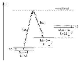
Figure 2: Sketch of a two-photon Raman transition between hyperfine levels, adapted from Spielman et al. Spielman2009 ; LinSpielman2009 .

For every two-photon transition the atom experiences a net change in its centre of mass angular momentum of $\Delta\ell=\ell_{1}-\ell_{2}$, while the change in linear momentum can be neglected. Hence there exists a coupling between $|M_{F}=-1,\ell-\Delta\ell\rangle$ and $|M_{F}=0,\ell\rangle$ as well as between $|M_{F}=0,\ell\rangle$ and $|M_{F}=+1,\ell+\Delta\ell\rangle$. The two light beams are slightly detuned from the Raman two-photon resonance, with detuning $\delta\equiv(\omega_{1}-\omega_{2})-Z/\hbar$. Including the kinetic energies of the different angular momentum states and applying the rotating wave approximation Spielman2009 , one arrives at the full Hamiltonian, $\hat{H}(\ell)/\hbar$,

$$\left(\begin{array}[]{ccc}\frac{\hbar}{2MR^{2}}(\ell+\Delta\ell)^{2}-\delta&\Omega_{R}/2&0\\ \Omega_{R}/2&\frac{\hbar}{2MR^{2}}\ell^{2}&\Omega_{R}/2\\ 0&\Omega_{R}/2&\frac{\hbar}{2MR^{2}}(\ell-\Delta\ell)^{2}+\delta\end{array}\right).$$ (9)

The $\ell$ dependence has been made explicit; each atomic state is defined by the amplitudes of the three hyperfine states and its angular momentum $\ell$. Here $\Omega_{R}$ is the two-photon Rabi frequency which describes the coupling between hyperfine states. The effect of the Zeeman splitting is given by $\delta$ footnote1 . For each $\ell$ there are three energy eigenvalues of (9), corresponding to three dressed energy bands.

In Fig. 3, we show the results of a numerical diagonalization of the Hamiltonian (9).

Figure 3: Coupled (solid lines) and uncoupled (dashed lines) energy bands of a three-level system, from Ref. CooperHadzibabic2010, , with the parameter $\delta=0.5\hbar(\Delta\ell)^{2}/MR^{2}$. The smooth curves interpolate between the allowed integer values of $\ell$.

The three uncoupled energy levels for $\Omega_{R}=0$ are shown as dotted lines. When the light is on, $\Omega_{R}\neq 0$, these levels are mixed and lead to the energy levels of the dressed states (solid lines). For non-zero detuning $\delta$ the minimum of the lowest band is displaced to a non-zero angular momentum $\ell^{*}$. Provided that all atoms are restricted to states in the lowest-energy dressed band, the atoms experience an effective dispersion relation of the form (2) in which the non-zero $\ell^{*}$ plays the role of an azimuthal gauge field.

Throughout this paper, we assume that only this lowest dressed band is occupied. This is justified if the chemical potential $\mu$ and temperature $kT$ are small compared to the band splitting, which is of order $\hbar\Omega_{R}$. Hence we require that $\Omega_{R}$ be sufficiently large. The lowest band will be referred to as $\epsilon^{0}_{\parallel}(\ell)$ in Section V. To obtain the results shown in Section VI, we determine $\epsilon^{0}_{\parallel}(\ell)$ by numerical solution of (9). However, to allow an understanding of the general trends, we derive some analytic expressions which are valid for large $\Omega_{R}$, where the bands are far apart from each other and the lowest band is nearly parabolic. Perturbation theory in $1/\Omega_{R}$ shows CooperHadzibabic2010 that the minimum of the dispersion relation is shifted from $\ell=0$ to

$$\ell^{*}\simeq-\sqrt{2}\frac{\delta}{\Omega_{R}}\Delta\ell+{\cal O}(1/\Omega_{R}^{2})\,,$$ (10)

and the bare mass is increased to an effective mass $M^{*}$, with

$$M^{*}\simeq M\left(1+\frac{\sqrt{2}\hbar(\Delta\ell)^{2}}{MR^{2}\Omega_{R}}\right)+{\cal O}(1/\Omega_{R}^{2}).$$ (11)

Similarly, perturbative calculations of $\left|\psi_{-1}(\ell)\right|^{2}$ and $\left|\psi_{+1}(\ell)\right|^{2}$ show that they have equal and opposite contributions linear in $\ell$. The difference $\left|\psi_{-1}(\ell)\right|^{2}-\left|\psi_{+1}(\ell)\right|^{2}$ can indeed be written as a series in $\ell$, as in Eq. (6), with

$$\Delta p_{0} \simeq\frac{\delta}{\Omega_{R}}\left[\sqrt{2}-\frac{\hbar(\Delta\ell)^{2}}{MR^{2}\Omega_{R}}\right]+{\cal O}(1/\Omega_{R}^{3}),$$ (12)

$$\Delta p^{\prime} \simeq-\sqrt{2}\frac{\hbar\Delta\ell}{MR^{2}\Omega_{R}}+{\cal O}(1/\Omega_{R}^{2}).$$ (13)

As parameters representative of experiments, throughout this paper we consider sodium with $M=23\,m_{p}$ (where $m_{p}$ is the proton mass) in a trap of radius $R=10\,\mathrm{\mu m}$. A typical value of the effective mass is $M^{*}\approx 1.15M$ (at a two-photon Rabi frequency $\Omega_{R}=2\pi\times 100\,\mathrm{kHz}$ and for $\Delta\ell=50$).

IV Corrections

In the preceding sections, we have summarised the theoretical proposal of Ref. CooperHadzibabic2010, . This showed how to relate the superfluid fraction to a spectroscopically determined hyperfine population imbalance [see Eq. (8)]. The quantitative accuracy of this relation relies on the validity of the termination of the Taylor expansions in Eqs. (2) and (6) at quadratic and linear orders respectively. If these (terminated) expansions were exact, the superfluid fraction would be perfectly determined by Eq. (8). In practice, higher-order corrections do exist, i.e.

$$E =E_{\textrm{parabolic}}+c\ell^{3}+\dots$$ (14)

$$\Delta p_{\ell} =(\Delta p_{\ell})_{\textrm{linear}}+c^{\prime}\ell^{2}+\dots$$ (15)

where $E_{\textrm{parabolic}}$ and $(\Delta p_{\ell})_{\textrm{linear}}$ correspond to the lower-order expansions (2) and (6).

The higher-order corrections have two major implications.

Firstly, corrections to $\Delta p_{\ell}$ of quadratic or higher order in $\ell$ lead to a deviation of the spectroscopic measurement [the right-hand side of Eq. (7)] from the actual average angular momentum $\langle\ell\rangle$.

Secondly, corrections to the effective kinetic energy $E$ of cubic or higher order in $\ell$ mean that even the very definition of the superfluid fraction, Eq. (1), breaks down. A basic assumption of this definition is that the rotational properties of a (normal) gas are entirely characterised by its moment of inertia. This is correct provided the kinetic energy is a quadratic function of the angular momentum. Then, under a transformation to a frame rotating at angular frequency ${\bm{\omega}}$, the interaction energy is unchanged, and the (parabolic) kinetic energy transforms as $E\to E^{\prime}=E+{\bm{\omega}}\cdot\langle{\bm{L}}\rangle+\frac{1}{2}I_{\textrm{cl}}\omega^{2}$. Thus, for a state of given average angular momentum, the only material property characterising the net energy change is the moment of inertia $I_{\textrm{cl}}$. For non-parabolic kinetic energy, however, the kinetic energy does not transform in any simple way, but depends on the populations of the individual angular momentum states and hence also on how interactions and/or temperature have distributed particles among these levels. The moment of inertia of even a normal gas cannot be assumed simply to be a constant $I_{\textrm{cl}}$.

We now turn to estimate the quantitative effects of these two forms of correction.

First we consider the effects of the higher-order corrections to $\Delta p_{\ell}$, Eq. (15). Because of the departure of $\Delta p_{\ell}$ from its linear expansion, we find $\Delta p^{\prime}\ell^{*}\neq\Delta p_{\ell^{*}}-\Delta p_{0}$. This difference is illustrated for different combinations of $\Omega_{R}$ and $\Delta\ell$ in Fig. 4, where the dashed lines show $\Delta p^{\prime}\ell^{*}$ and the circles show the actual difference $\Delta p_{\ell^{*}}-\Delta p_{0}$. As a consequence, Eq. (8) would give a systematically incorrect result even in the $T\to 0$ limit. In practice this can be corrected by replacing the denominator in (8) by $\Delta p_{\ell^{*}}-\Delta p_{0}$.

A more serious problem arises from the fact that non-zero temperature and/or interactions populate a range of $\ell$ states. Due to this broadening of the distribution function, the higher-order corrections to $\Delta p_{\ell}$ in Eq. (15) lead to the situation that for a normal gas (or a relaxed superfluid) with average momentum $\langle\ell\rangle=\ell^{*}$, the spectroscopic signal $\Delta p$ is not just determined by the signal of the state at $\ell^{*}$, but depends on the overall distribution function, so $\Delta p\neq\Delta p_{\ell^{*}}$. Similarly, for the (metastable) superfluid with $\langle\ell\rangle=0$, one has $\Delta p\neq\Delta p_{0}$. Hence one would incorrectly determine the superfluid fraction. In order to estimate the size of this error, we here consider the effect of temperature using the example of an ideal Boltzmann gas. (Interactions will be considered in Sections V and VI.) We populate the different $\ell$ states in the lowest band (see Fig. 3) according to a Boltzmann distribution $n_{\ell}\propto\exp[-\epsilon^{0}_{\parallel}(\ell)/kT]$. The results are shown for a range of temperatures by the solid lines in Fig. 4. If the effects of thermal broadening were negligible, all these curves would agree with $\Delta p_{\ell^{*}}-\Delta p_{0}$ (the circles in Fig. 4).

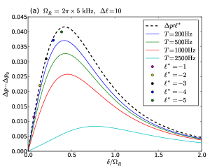
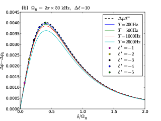
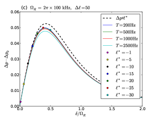
Figure 4: (Color online) Results for a normal gas: Ideal signal size $\Delta p^{\prime}\ell^{*}$ and temperature-dependent deviation from this as a function of the detuning, $\delta/\Omega_{R}$. Data are for a classical Boltzmann gas at several values of $\Omega_{R}$ and $\Delta\ell$. Circles denote the zero-temperature limit $(\Delta p_{\ell^{*}}-\Delta p_{0})$ at different values of $\ell^{*}$. The curves are labelled from top to bottom, and $\ell^{*}$ is labelled from left to right.

Increasing $\Omega_{R}$ decreases the relevance of higher-order corrections, but also diminishes the signal size $\Delta p^{\prime}\ell^{*}$ and thus leads to a bigger experimental uncertainty. Increasing $\Delta\ell$ has the opposite effect. One goal of this paper is to find parameters for which a good compromise can be reached, such that there is both a large experimental signal and small systematic inaccuracies.

For $\delta/\Omega_{R}\ll 1$, the influence of $\Omega_{R}$ and $\Delta\ell$ on signal strength and higher-order corrections can be seen in the expressions from perturbation theory. Using the perturbative expansions in $1/\Omega_{R}$ (cf. Section III), the signal size is given by

$$\Delta p^{\prime}\ell^{*}\simeq 2\frac{\delta}{\Omega_{R}}\frac{\hbar}{MR^{2}\Omega_{R}}(\Delta\ell)^{2}+{\cal O}(1/\Omega_{R}^{3}),$$ (16)

and considering the corrections to $\Delta p_{\ell}$ in (15), the second-order coefficient $c^{\prime}$ is given by

$$c^{\prime}\simeq-3\sqrt{2}\frac{\delta}{\Omega_{R}}\left(\frac{\hbar}{MR^{2}\Omega_{R}}\right)^{2}(\Delta\ell)^{2}+{\cal O}(1/\Omega_{R}^{4}).$$ (17)

These expressions show that increasing $\Delta\ell$ is an effective way to increase the signal size, but also has an adverse effect on the accuracy. Accuracy is improved by increasing $\Omega_{R}$, but at a reduction in signal size. As a trade-off one would thus try to make $\Delta\ell$ as high as possible, and then increase $\Omega_{R}$ as long as the signal size remains big enough. As a reasonable, and experimentally feasible, compromise we choose $\Delta\ell=50$ and $\Omega_{R}=2\pi\times 100\,\mathrm{kHz}$ [as in Fig. 4 (c)]. These are the values we will use through the remainder of this paper.

Second, and finally, we return to the definition of superfluidity in Eq. (1), and estimate its adequacy. Measuring the relative deviation $(\langle\ell\rangle-\ell^{*})/\ell^{*}$ is a way to assess the departure from parabolicity due to the terms of $E$ which are odd in $\ell$. For the Boltzmann gas of Fig. 4, the relative deviation is maximal at $\ell^{*}\sim\delta\to 0$ (with a maximum value $\propto 1/\Omega_{R}^{2}$) and decreases with higher $\delta$. At $T=1000\,\mathrm{Hz}$ footnotet , the maximum value of the deviation at $\delta\to 0$ is about $0.3\%$. To further quantify the size of non-parabolic corrections to the dispersion relation, we have carried out fourth-order perturbation theory Fernandez2001 in $1/\Omega_{R}$. The next terms in the series in $\ell$ are

$$E\simeq E_{\textrm{parabolic}} -\sqrt{2}\frac{\delta}{\Omega_{R}}\frac{\hbar^{4}(\Delta\ell)^{3}}{(MR^{2})^{3}\Omega_{R}^{2}}\ell^{3}$$

$${}+\frac{1}{2\sqrt{2}}\frac{\hbar^{5}(\Delta\ell)^{4}}{(MR^{2})^{4}\Omega_{R}^{3}}\ell^{4}+{\cal O}(\ell^{5}),$$ (18)

where both coefficients have higher-order contributions of ${\cal O}(1/\Omega_{R}^{4})$. The contributions of cubic and quartic term relative to the parabolic term ($\hbar^{2}\ell^{2}/2M^{*}R^{2}$) are of order $10^{-4}\ell\,$ and $10^{-7}\ell^{2}$, respectively. This is on the same order as the $0.3\%$ estimated above: For $T=1000\,\mathrm{Hz}$ and $\ell^{*}=1$, the root mean square angular momentum is $\sqrt{\langle\ell^{2}\rangle}\sim 16$, so we would expect the relative correction due to the cubic term to be about $0.2\%$. This deviation of the dispersion relation from parabolicity sets an upper bound to the accuracy with which one can determine the superfluid fraction.

V Interactions

In addition to the effects of non-zero temperature on a normal fluid, we want to know what happens to $\Delta p$ due to interactions in a superfluid. It is important to note that a gas is only superfluid because of interactions; in the limit of vanishing interaction strength, the critical velocity (see below, Section V.3) goes to zero, so a metastable superfluid flow cannot be maintained.

Here we do not attempt a full model of the interacting gas in a trap. Rather, we aim to use a method that includes interactions in the simplest way. We therefore consider an interacting gas with uniform density. The density inhomogeneity near the walls is on the scale of the healing length $\xi=(8\pi na)^{-1/2}$, which is the distance over which the condensate recovers its bulk value from zero density at the walls. We assume that $\xi\ll\Delta R$ and that we can thus neglect the density inhomogeneity. We therefore model the gas in a ring-like trap by considering a torus of radius $R$ and with a rectangular cross-sectional area $A=L\times L$, cf. Fig. 5.

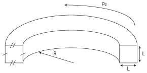
Figure 5: The system geometry employed in this section, a toroidal trap with hard walls and a cross-sectional area $L\times L$. For the radius $R\gg L$, angular momentum $\ell$ can be unrolled unto the $p_{z}$ direction, $p_{z}=\hbar\ell/R$, which then has effective periodic boundary conditions. Thus $\ell$ and $p_{z}$ will be used interchangeably.

Since we neglect density inhomogeneities, we consider the system to be uniform and impose periodic boundary conditions in the transverse directions. For $L\sim\Delta R\ll R$ we can unroll the angular momentum from the circumferential direction of the torus onto a line with periodic boundary conditions, equivalent to a linear momentum $p_{z}=(\hbar/R)\ell$, where $\ell$ is the angular momentum (in units of $\hbar$) defined above. With this understanding we will use $\ell$ and $p_{z}$ interchangeably.

We are only interested in the azimuthal motion, $p_{z}$ or $\ell$, in which we would like to measure superfluidity. Therefore we will integrate out the two transverse directions ${\bm{p}}_{\perp}$. These have a simple kinetic energy dispersion, $p_{\perp}^{2}/2M$. In the azimuthal direction we allow for a general dispersion relation $\epsilon^{0}_{\parallel}(p_{z})$, set by the energy of the lowest band of the Hamiltonian (9). The total dispersion relation is given by

$$\epsilon^{0}({\bm{p}})=\frac{1}{2M}{\bm{p}}_{\perp}^{2}+\epsilon_{\parallel}^{0}(p_{z}).$$ (19)

Later on we will compare the superfluid fraction with the condensate fraction, so it is instructive to determine the number of excited particles $N_{\textrm{ex}}$. Here, we will determine this for an ideal non-interacting gas, as many of the features will carry over to the interacting case discussed below. In a non-interacting gas the number of excited particles is given by

$$N_{\text{ex}}=\sum_{{\bm{p}}\neq 0}n_{B}\left(\epsilon^{0}({\bm{p}})\right),$$ (20)

where $n_{B}(\epsilon)=[\exp(\epsilon/kT)-1]^{-1}$ is the Bose-Einstein distribution in the condensed system (for which the chemical potential vanishes, $\mu=0$). We split the sum,

$$N_{\text{ex}}=N_{\text{ex}}^{\perp}(p_{z}=0)+\sum_{p_{z}\neq 0}N_{\text{ex}}^{\perp}(p_{z}),$$ (21)

defining

$$N_{\text{ex}}^{\perp}(p_{z})\equiv\sum_{{\bm{p}}_{\perp}\neq 0}n_{B}\left({\bm{p}}_{\perp}^{2}/2M+\epsilon_{\parallel}^{0}(p_{z})\right).$$ (22)

Here we assume without loss of generality that the energy minimum is at $\epsilon_{\parallel}^{0}(p_{z}=0)=0$. We switch to an integral representation according to $\sum_{p}\to\frac{L}{2\pi\hbar}\int dp$. The term $N_{\textrm{ex}}^{\perp}(p_{z})$ with $p_{z}\neq 0$ does not pose any problems. However, when evaluating the $p_{z}=0$ contribution, we find

$$N_{\text{ex}}^{\perp}(p_{z}=0) =\frac{A}{(2\pi\hbar)^{2}}\int d^{2}{\bm{p}}_{\perp}n_{B}({\bm{p}}_{\perp}^{2}/2M)$$

$$=\frac{2\pi A}{(2\pi\hbar)^{2}}\int_{0}^{\infty}dp\,p\,n_{B}(p^{2}/2M),$$ (23)

which is infrared divergent. For $p\to 0$, the integrand is approximately given by $p/(p^{2}/2M\,kT)\sim 1/p$, thus the indefinite integral at small momenta is $\sim-\log(p_{\rm min})$. Fortunately, in the thermodynamic limit this logarithmic divergence is unproblematic. Noting that the low-momentum cut-off is $p_{\text{min}}\sim\frac{1}{L}$, one finds $N_{\text{ex}}^{\perp}(p_{z}=0)\sim(A/\lambda_{T}^{2})\log(L/\lambda_{T})$, where $\lambda_{T}$ is the thermal de Broglie wavelength. The other contributions are extensive, $N_{\text{ex}}^{\perp}(p_{z}\neq 0)\sim(V/\lambda_{T}^{3})$, so

$$\frac{N_{\text{ex}}^{\perp}(p_{z}=0)}{N_{\text{ex}}^{\perp}(p_{z}\neq 0)}\sim\frac{\lambda_{T}}{R}\log(L/\lambda_{T}),$$ (24)

and $N_{\text{ex}}^{\perp}(p_{z}=0)$ can be neglected in the limit $\lambda_{T}\ll R$. The same reasoning applies when taking interactions into account, so from now on we will drop the $p_{z}=0$ contribution to $N_{\text{ex}}$ and replace $\sum_{{\bm{p}}\neq 0}$ by $\sum_{p_{z}\neq 0}\sum_{{\bm{p}}_{\perp}\neq 0}$.

V.1 Weak interactions with asymmetric dispersion

In the following we consider an interacting gas, with a general, possibly asymmetric, non-interacting dispersion relation $\epsilon^{0}({\bm{p}})$. Since we study atoms in the ultracold limit, all interactions can be treated as contact interactions, $U_{\text{eff}}({\bm{r}},{\bm{r^{\prime}}})=U_{0}\delta({\bm{r}}-{\bm{r^{\prime}}})$. Here we take $U_{0}=4\pi\hbar^{2}a/M$, assuming for simplicity that the scattering length $a$ is independent of the internal state. The Hamiltonian in the momentum basis is

$$\hat{H}= \sum_{i,{\bm{p}}}\epsilon_{i,{\bm{p}}}^{0}\hat{a}_{i,{\bm{p}}}^{+}\hat{a}_{i,{\bm{p}}}$$

$${}+\frac{1}{2V}U_{0}\sum_{ijkl}\sum_{{\bm{p}},{\bm{p}}^{\prime},{\bm{q}}}\hat{a}_{i,{\bm{p}}+{\bm{q}}}^{+}\hat{a}_{j,{\bm{p}}^{\prime}-{\bm{q}}}^{+}\hat{a}_{k,{\bm{p}}^{\prime}}\hat{a}_{l,{\bm{p}}}.$$ (25)

The indices $i,j,k,l$ stand for internal states, e.g. one of the three hyperfine bands. As we assume that only the lowest band is occupied (cf. Section III), we can ignore inter-band mixing and simplify Eq. (25) to the Hamiltonian we will consider hereafter:

$$\hat{H}=\sum_{{\bm{p}}}\epsilon^{0}({\bm{p}})\hat{a}_{{\bm{p}}}^{+}\hat{a}_{{\bm{p}}}+\frac{U_{0}}{2V}\sum_{{\bm{p}},{\bm{p}}^{\prime},{\bm{q}}}\hat{a}_{{\bm{p}}+{\bm{q}}}^{+}\hat{a}_{{\bm{p}}^{\prime}-{\bm{q}}}^{+}\hat{a}_{{\bm{p}}^{\prime}}\hat{a}_{{\bm{p}}}.$$ (26)

V.1.1 Bogoliubov transformation

We assume that the condensate has only one macroscopically occupied state ${\bm{p}}_{c}=0$. Should the condensate be in a state ${\bm{p}}_{c}\neq 0$, we can shift all momenta by relabelling the states to ${\bm{p}}^{\prime}\equiv{\bm{p}}-{\bm{p}}_{c}$ with energy $\epsilon^{0\prime}({\bm{p}}^{\prime})=\epsilon^{0}({\bm{p}}_{c}+{\bm{p}}^{\prime})$. We note that, for a superfluid, the state ${\bm{p}}_{c}$ is not necessarily the ground state: for example, as in the protocol described above, a superfluid may remain condensed in $\ell=0$ even after a gauge field is applied such that the lowest-energy single particle state has $\ell^{*}\neq 0$. Our discussion in this section also applies to these metastable superfluid states.

The creation and annihilation operators of the ground state are $\hat{a}_{0}^{+}$ and $\hat{a}_{0}$, respectively. We have $\langle\hat{a}_{0}^{+}\hat{a}_{0}\rangle=N_{0}$, where $N_{0}$ is the number of particles in the condensate. For $N_{0}\gg 1$, we can therefore neglect the commutator $[\hat{a}_{0},\hat{a}_{0}^{+}]_{-}=1$ compared to the operator $\hat{a}_{0}^{+}\hat{a}_{0}$, and replace the ground state operators by a c-number: $\hat{a}_{0}\simeq\hat{a}_{0}^{+}\simeq\sqrt{N_{0}}$. Expanding the interaction term and only keeping terms of order $\mathcal{O}(N_{0})$ or higher (i.e. assuming the only relevant interactions are with the condensate state), one finds

$$\hat{H} \simeq N\epsilon^{0}(0)+\frac{U_{0}N^{2}}{2V}$$ (27)

$${}+\sum_{{\bm{p}}\neq 0}\left[\epsilon^{0}({\bm{p}})-\epsilon^{0}(0)+U_{0}n_{0}\right]\hat{a}_{{\bm{p}}}^{+}\hat{a}_{{\bm{p}}}$$

$${}+\frac{U_{0}n_{0}}{2}\sum_{{\bm{p}}\neq 0}\left(\hat{a}_{{\bm{p}}}^{+}\hat{a}_{-{\bm{p}}}^{+}+\hat{a}_{{\bm{p}}}\hat{a}_{-{\bm{p}}}\right)$$

$$= \sum_{{\bm{p}}\neq 0}^{\prime}\left\{[\epsilon^{0}({\bm{p}})-\epsilon^{0}(0)+\epsilon_{1}]\,\hat{a}_{{\bm{p}}}^{+}\hat{a}_{{\bm{p}}}\right.$$

$$\left.{}+[\epsilon^{0}(-{\bm{p}})-\epsilon^{0}(0)+\epsilon_{1}]\,\hat{a}_{-{\bm{p}}}^{+}\hat{a}_{-{\bm{p}}}\right\}$$

$${}+\sum_{{\bm{p}}\neq 0}^{\prime}\epsilon_{1}\left(\hat{a}_{{\bm{p}}}^{+}\hat{a}_{-{\bm{p}}}^{+}+\hat{a}_{{\bm{p}}}\hat{a}_{-{\bm{p}}}\right)+E_{\text{offset}},$$

where the prime on the sum denotes that we only sum over (an arbitrary) half of momentum space. Here $n_{0}\equiv N_{0}/V$ is the condensate density, and we have defined $\epsilon_{1}\equiv U_{0}n_{0}=4\pi\hbar^{2}an_{0}/M$, which sets the chemical potential, $\mu=\epsilon_{1}$. The constant terms have been absorbed into $E_{\text{offset}}$.

We diagonalize the Hamiltonian using the Bogoliubov transformation

$$\hat{\alpha}_{{\bm{p}}} :=u\hat{a}_{{\bm{p}}}+v\hat{a}_{-{\bm{p}}}^{+},$$

$$\hat{\alpha}_{-{\bm{p}}}\equiv\hat{\beta}_{{\bm{p}}} :=u\hat{a}_{-{\bm{p}}}+v\hat{a}_{{\bm{p}}}^{+},$$ (28)

with $[\hat{\alpha},\hat{\alpha}^{+}]_{-}=[\hat{\beta},\hat{\beta}^{+}]_{-}=u^{2}-v^{2}=1$. The Hamiltonian (27) is diagonalized by choosing $u^{2}=\frac{1}{2}\left(\frac{\bar{\epsilon}}{\epsilon}+1\right)$ and $v^{2}=\frac{1}{2}\left(\frac{\bar{\epsilon}}{\epsilon}-1\right)$, leading to

$$\hat{H}=E_{\text{offset}}+\sum_{{\bm{p}}\neq 0}\frac{1}{2}\left(\epsilon-\bar{\epsilon}\right)+\sum_{{\bm{p}}\neq 0}\underbrace{\left(\epsilon+\bar{\gamma}\right)}_{\epsilon_{\text{exc}}}\hat{\alpha}_{{\bm{p}}}^{+}\hat{\alpha}_{{\bm{p}}},$$ (29)

where $\epsilon_{\text{exc}}({\bm{p}})=\epsilon({\bm{p}})+\bar{\gamma}({\bm{p}})$ is the energy of Bogoliubov excitations. We have defined footnote3

$$\gamma({\bm{p}}) =\frac{1}{2}\left[\epsilon^{0}({\bm{p}})+\epsilon^{0}(-{\bm{p}})\right]-\epsilon^{0}(0),$$

$$\bar{\gamma}({\bm{p}}) =\frac{1}{2}\left[\epsilon^{0}({\bm{p}})-\epsilon^{0}(-{\bm{p}})\right],$$

$$\bar{\epsilon}({\bm{p}}) =\gamma({\bm{p}})+\epsilon_{1},$$

$$\epsilon({\bm{p}}) =\sqrt{\bar{\epsilon}^{2}-\epsilon_{1}^{2}}=\sqrt{\gamma(\gamma+2\epsilon_{1})}.$$ (30)

$\gamma({\bm{p}})$ denotes the symmetric part of the non-interacting dispersion relation, shifted such that $\gamma({\bm{p}}_{c})=0$. $\epsilon({\bm{p}})$ is the symmetric part of the Bogoliubov excitation energy. $\bar{\gamma}({\bm{p}})$ denotes the asymmetric part of the excitation energy, and is the same for both non-interacting and interacting cases. As opposed to the standard case of a symmetric dispersion relation, we find $\bar{\gamma}\neq 0$ and a dependence of the energy $\epsilon_{\textrm{exc}}$ of Bogoliubov excitations on $\ell^{*}$. We shall use this in Section V.3 to determine the critical velocity at which the metastable superfluid becomes unstable.

V.1.2 Depletion of the condensate

We can write the operator for the total number of particles as

$$\hat{N}=N_{0}+\sum_{{\bm{p}}\neq 0}\hat{a}_{{\bm{p}}}^{+}\hat{a}_{{\bm{p}}}.$$ (31)

When we apply the Bogoliubov transformation, we find

$$N\simeq N_{0}+\sum_{{\bm{p}}\neq 0}\frac{1}{2}\left(\frac{\bar{\epsilon}}{\epsilon}-1\right)+\sum_{{\bm{p}}\neq 0}\frac{\bar{\epsilon}}{\epsilon}\left\langle\hat{\alpha}_{{\bm{p}}}^{+}\hat{\alpha}_{{\bm{p}}}\right\rangle,$$ (32)

where we have already taken the expectation value. At zero temperature,

$$N(T=0)=N_{0}+\sum_{{\bm{p}}\neq 0}\frac{1}{2}\left(\frac{\bar{\epsilon}}{\epsilon}-1\right).$$ (33)

After changing the sum to an integral, we can analytically integrate out the transverse directions. In terms of the number density $n=N/V$ we get

$$n(T=0)=n_{0}+\frac{n_{0}a}{2\pi R}\sum_{p_{z}\neq 0}\left[1+\frac{\gamma}{\epsilon_{1}}\left(1-\sqrt{1+2\frac{\epsilon_{1}}{\gamma}}\right)\right],$$ (34)

where $\gamma$ is evaluated at ${\bm{p}}_{\perp}=0$; $\gamma=\gamma(p_{z};{\bm{p}}_{\perp}=0)$. Each term of the sum gives the corresponding $\ell$-state occupation $n_{\ell}(T=0)$.

To find the temperature-dependent depletion, we calculate the expected excitation number: $\langle\hat{\alpha}_{{\bm{p}}}^{+}\hat{\alpha}_{{\bm{p}}}\rangle=n_{B}\left(\epsilon_{\text{exc}}({\bm{p}})\right)$. The energy of such thermal excitations is given by $\epsilon_{\textrm{exc}}=\epsilon+\bar{\gamma}$. Changing the integral over transverse directions into an integration over the dimensionless $x=p_{\perp}^{2}/(2M\epsilon_{1})$ leads to

$$n(T)-n(T=0)$$

$$=\frac{n_{0}a}{\pi R}\sum_{p_{z}\neq 0}\int_{0}^{\infty}dx\frac{x+1+\gamma/\epsilon_{1}}{\sqrt{(x+1+\gamma/\epsilon_{1})^{2}-1}}\times$$

$$\quad\times\frac{1}{\exp\left[\left(\epsilon_{1}\sqrt{(x+1+\gamma/\epsilon_{1})^{2}-1}+\bar{\gamma}\right)/kT\right]-1},$$ (35)

again with $\gamma=\gamma(p_{z};{\bm{p}}_{\perp}=0)$. In general, this integral has to be evaluated numerically. Similarly to above, the terms of this sum give the finite-temperature distribution function $n_{\ell}(T)-n_{\ell}(T=0)$.

V.2 Popov approximation

To extend the validity of our approximation to higher temperatures, we employ the Popov approximation. In the homogeneous system, the Popov approximation leads to the same Hamiltonian as in the Bogoliubov theory, except for a simple excitation-independent energy offset. Thus the distribution function stays the same — the only difference is that now we need to determine $n_{0}$ self-consistently, both at zero and at non-zero temperature PethickSmith2008 ; Popov1988Functional .

As the zero-temperature distribution (34) is symmetric around $\ell=0$, at $T=0$ the average angular momentum is always zero, $\langle\ell\rangle\equiv 0$, for any interaction strength. This recovers the expectation that $\rho_{s}/\rho=1$ even if the condensate is depleted by interactions. We calculate the zero-temperature depletion for a parabolic dispersion relation $\epsilon^{0}_{\parallel}=\frac{\hbar^{2}\ell^{2}}{2MR^{2}}=\gamma$. We approximate the sum in Eq. (34) by an integral,

$$\frac{n-n_{0}}{n_{0}}=\frac{a}{2\pi R}\frac{2\pi R}{2\pi\hbar}\int_{0}^{\infty}dp_{z}\left[1+\frac{\gamma}{\epsilon_{1}}\left(1-\sqrt{1+2\frac{\epsilon_{1}}{\gamma}}\right)\right],$$ (36)

which can be evaluated analytically, giving

$$\frac{n-n_{0}}{n_{0}} =\frac{a\sqrt{2M}}{2\pi\hbar}\sqrt{\frac{4\pi\hbar^{2}an_{0}}{M}}\left(+\frac{4}{3}\sqrt{2}\right)$$

$$=\frac{8}{3\sqrt{\pi}}\left(n_{0}a^{3}\right)^{1/2},$$ (37)

where we substituted $\epsilon_{1}=4\pi\hbar^{2}an_{0}/M$. The resulting expression for the condensate fraction,

$$\frac{n_{0}}{n}\simeq\left[1+\frac{8}{3\sqrt{\pi}}\left(n_{0}a^{3}\right)^{1/2}\right]^{-1},$$ (38)

is not in a closed form; we have to find a self-consistent solution for $n_{0}$ numerically. At small depletions $n_{\textrm{ex}}/n\ll 1$, Eq. (38) simplifies to the Bogoliubov result PethickSmith2008 , $n_{0}/n\simeq 1-\frac{8}{3\sqrt{\pi}}(na^{3})^{1/2}$.

According to this theory, one would simply occupy the lowest band as stated in the interacting distribution function given by Eq. (35) until convergence is achieved. For a parabolic dispersion relation, Eq. (35) has an asymptotic behaviour $n_{\ell}\propto 1/\ell^{2}$ at large momenta, $\ell\gg 1$, and thus extends to very high $\ell$. However, the physical distribution of atoms does not extend beyond $\ell_{\textrm{max}}\sim R/R_{e}$, where $R_{e}$ is the range of the interaction potential (in practical terms, this is of the same order as the scattering length $a$). Thus we do not trust the expression for $n_{\ell}$, Eq. (35), for $\ell/R\gtrsim 1/R_{e}\sim 1/a$, and so it is pointless to do the whole sum. In any case, all the important physics characterising the superfluid response is contained in $p\lesssim\hbar/\xi$ (equivalent to $\ell\lesssim R/\xi$). Hence we introduce a cut-off by ignoring states with $\ell>\ell_{\rm cut}$. We choose $\ell_{\rm cut}\sim 10\times 2\pi R/\xi$, for which the relative error in $\Delta p^{\mathrm{RSF}}-\Delta p^{\mathrm{SF}}$ due to the cut-off with respect to $\ell_{\textrm{cut}}=\infty$ is on the order of $10^{-4}$.

V.3 Critical velocity

In order that the system is (meta)stable, the minimum of the excitation energy $\epsilon_{\text{exc}}=\epsilon+\bar{\gamma}$ has to be positive: $\min_{\ell}\epsilon_{\text{exc}}(\ell)>0$. This leads to a critical angular momentum shift $\ell^{*}_{\textrm{crit}}$ above which, for $|\ell^{*}|>\ell^{*}_{\textrm{crit}}$, the superfluid flow is unstable. (This is the Landau criterion for stable superfluid flow.) The determination of the critical $\ell^{*}$ in the general case requires a full (numerical) determination of the dispersion relation of the lowest dressed band, $\epsilon^{0}_{\parallel}(p_{z})$. In the limit in which the non-interacting dispersion relation can be taken to be parabolic [cf. Eq. (2)], the symmetric and antisymmetric parts of $\epsilon^{0}_{\parallel}$ are given by $\gamma(\ell)=\frac{\hbar^{2}}{2M^{*}R^{2}}\ell^{2}$ and $\bar{\gamma}(\ell)=-\frac{\hbar^{2}\ell^{*}}{M^{*}R^{2}}\ell$. Then the lowest-energy Bogoliubov excitation at given $\ell$ is

$$\epsilon_{\rm exc}({\bm{p}}_{\perp}=0)=\epsilon+\bar{\gamma}\simeq\sqrt{\frac{\hbar^{2}\epsilon_{1}}{M^{*}R^{2}}}|\ell|-\frac{\hbar^{2}\ell^{*}}{M^{*}R^{2}}\ell\,.$$ (39)

This is positive for all $\ell$ only if

$$\hbar^{2}|\ell^{*}|/M^{*}R^{2}<\sqrt{\hbar^{2}\epsilon_{1}/M^{*}R^{2}}\,.$$

Substituting $\epsilon_{1}=4\pi\hbar^{2}an_{0}/M$, this corresponds to

$$|\ell^{*}|<\ell^{*}_{\rm crit}=\sqrt{4\pi R^{2}an_{0}\frac{M^{*}}{M}}\,.$$ (40)

If $|\ell^{*}|<\ell^{*}_{\rm crit}$, then $\epsilon_{\rm exc}(\ell)>0$ for all $\ell$. On the other hand, if $|\ell^{*}|>\ell^{*}_{\rm crit}$, then there always is some $\ell$ such that $\epsilon_{\rm exc}(\ell)<0$ and hence the system is thermodynamically unstable. It will relax due to the introduction of vortices. Eq. (40) shows that the metastable superfluid will become unstable when the condensate density is too low (i.e. when the temperature is too high), when interactions are too weak, or when $\ell^{*}$ is too large.

VI Results

In order to present the results of our calculations for an interacting gas, we consider two scenarios. In the first one, we study a Bose-Einstein condensate (BEC) with weak interactions, Section VI.1, for which we show that the proposed measurement technique gives the expected feature that the superfluid density and condensate density are almost the same. In the second scenario, Section VI.2, we turn to the more interesting case of a BEC with strong interactions, for which the condensate fraction and superfluid fraction are significantly different from each other. We show that the measurement protocol can distinguish the superfluid fraction from the condensate fraction. Finally, we will analyse the trade-off between signal strength and accuracy in Section VI.3.

As described above, in our studies the condensate is assumed to be uniform and boundary effects are neglected. When discussing temperature dependences, we shall also assume that the density $n$ is kept constant. For a harmonically trapped gas, with falling temperature the peak density quickly rises by more than an order of magnitude from near the transition point to when most of the atoms are in the condensate. We ignore this effect, since we are primarily interested in the low temperature properties of the BEC and less in the behaviour around the transition point. In the results we present, we choose the following parameters: $M=23\,m_{p}$, $R=10\,\mathrm{\mu m}$, $\Omega_{R}=2\pi\times 100\,\mathrm{kHz}$, $\Delta\ell=50$, and $n=10^{14}\,\mathrm{cm^{-3}}$. These are typical parameters achievable with current technology.

VI.1 Weakly interacting BEC

For a new experimental technique, it is important to establish that it works in a situation where the result is known. To that end, it will be valuable to see the results for a weakly interacting BEC, which can be well described by mean-field theories. Here we present the signal that one can expect to measure in such an experiment, for a weakly interacting BEC with $na^{3}=10^{-4}$. The condensate fraction at $T=0$ is approximately $99\%$, showing negligible depletion.

As described in Section II, the appearance of superfluidity displays a clear qualitative signal in this measurement technique. The processes of cooling and of imposing non-zero gauge field $\ell^{*}$ do not “commute” for a superfluid, so its response is hysteretic. First introducing $\ell^{*}$ (by increasing the Raman detuning $\delta$) and then cooling the gas leads to a condensate in the new ground state, $\ell_{c}=\ell^{*}$. This is the “relaxed superfluid” (RSF), with spectroscopic signal $\Delta p^{\mathrm{RSF}}$. On the other hand, cooling to below the transition point at $\ell^{*}=\delta=0$ creates the superfluid in $\ell_{c}=0$. Subsequently increasing $\delta$ leads to a metastable (non-relaxed) superfluid (SF), with spectroscopic signal $\Delta p^{\mathrm{SF}}$. Hence it is possible to measure two separate curves, $\Delta p^{\mathrm{RSF}}$ respectively $\Delta p^{\mathrm{SF}}$. In contrast, for a normal fluid, cooling and increasing $\delta$ do commute.

In Fig. 6 (a), we show the spectroscopic signatures of the metastable superfluid ($\Delta p^{\mathrm{SF}}$) and the relaxed superfluid ($\Delta p^{\mathrm{RSF}}$) at temperatures below the BEC transition temperature $T_{c}$. (The raw signal has been scaled by $\ell^{*}$ so that the numbers are of the same order.) One can see that the curves of the metastable superfluid ($\Delta p^{\mathrm{SF}}$) terminate at certain temperatures. This termination happens at a temperature (below the transition temperature) when the condensate becomes sufficiently depleted so that $|\ell^{*}|>\ell^{*}_{\textrm{crit}}$. Thus curves with higher $|\ell^{*}|$ break off at lower temperatures. The difference in the signals $\Delta p^{\mathrm{RSF}}\neq\Delta p^{\mathrm{SF}}$ below this temperature is a clear signature of the metastable superfluid flow.

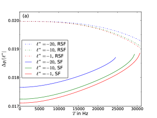
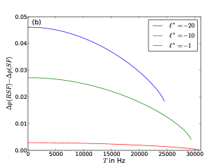
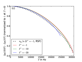
Figure 6: (Color online) Qualitative behaviour of the proposed superfluidity measurement as a function of temperature (in terms of the ideal gas transition temperature $T_{c}\approx 31.1\,\mathrm{kHz}$) at $na^{3}=10^{-4}$: (a) the raw $\Delta p$ signal scaled by $|\ell^{*}|$; (b) difference signal $\Delta p^{\mathrm{RSF}}-\Delta p^{\mathrm{SF}}$; (c) difference signal normalised to $1$ at $T=0$, and comparison with the condensate fraction $n_{0}/n$. Curves break off due to reaching $|\ell^{*}|>\ell^{*}_{\textrm{crit}}\simeq\sqrt{4\pi R^{2}an_{0}}$. The curves are labelled from top to bottom.

In order to extract a quantitative measure of the superfluid fraction from these results, one could take the curves for the metastable superfluid $\Delta p^{\mathrm{SF}}$ and use these in Eq. (8). Application of Eq. (8) requires knowledge of $\Delta p_{0}$ and $\Delta p^{\prime}$. As we have discussed, the result will also include some quantitative corrections from higher-order terms in the Taylor expansions of $E_{\ell}$ and $\Delta p_{\ell}$ (15). In view of these facts, it is helpful to take the difference $\Delta p^{\mathrm{RSF}}-\Delta p^{\mathrm{SF}}$. This removes the dependence on $\Delta p_{0}$ and also removes additive systematic errors. The differences $\Delta p^{\mathrm{RSF}}-\Delta p^{\mathrm{SF}}$ are shown in Fig. 6 (b). Finally, we scale these differences by the value of the same quantity that is obtained at $T=0$ for a weakly interacting gas,

$$\Delta p^{\mathrm{RSF}}(T=0,na^{3}\approx 0)-\Delta p^{\mathrm{SF}}(T=0,na^{3}\approx 0)\,.$$

[Since here we consider $na^{3}=10^{-4}$, this is almost identical to scaling by the $T=0$ limit of the curves in Fig. 6 (b).] These measurements are for states in which we know the system should be completely condensed and perfectly superfluid at $T=0$. They provide a direct measurement of the quantity $\Delta p^{\prime}\ell^{*}$, while also removing some multiplicative systematic errors.

The final scaled curves are shown in Fig. 6 (c). These show what the spectroscopic measurement would give for the superfluid fraction of the weakly interacting BEC as a function of temperature. The different values of $\ell^{*}$ correspond to different effective rotation rates. For comparison, the dashed line shows the numerically determined condensate fraction $n_{0}/n$ footnote2 . In this case, of a weakly interacting BEC, it is expected that the condensate and superfluid fractions should coincide. Fig. 6 (c) shows that this result is recovered to a very good accuracy by the spectroscopic measurement of the superfluid fraction. Furthermore, in a practical experimental measurement with a harmonically trapped gas we expect to find even better agreement between the spectroscopic measurement and $\rho_{s}/\rho$: here we chose $n=10^{14}\,\mathrm{cm^{-3}}$, which is a representative value for the density in the BEC, but this leads to a transition temperature which is several times higher than that found in experiments. In a typical experiment, the density would vary such that $T_{c}$ is lower, so $kT/\hbar\Omega_{R}$ would be smaller and quantitative corrections should have less of an effect.

VI.2 Strongly interacting BEC

We will now consider how the spectroscopic method can be used to provide an accurate quantitative measurement of the superfluid fraction in a regime where the condensate fraction $n_{0}/n$ and the superfluid fraction are significantly different. To this end, we shall consider a relatively strongly interacting BEC, with an interaction parameter up to $na^{3}=0.1$. We cannot trust Popov theory to be an accurate quantitative theory of an atomic gas in regimes of strong interactions. However, we can still use the results of Popov theory to assess the accuracy of the spectroscopic method of measuring the superfluid fraction. Specifically, we know that, even for a strongly interacting gas, in the low temperature limit the superfluid fraction should be $\rho_{s}/\rho=1$, while the condensate fraction can be significantly depleted. Here we wish to demonstrate that the difference between condensate fraction and superfluid fraction can be observed using the spectroscopic measurement method.

As described in Section IV, while considering an accurate quantitative measurement of $\rho_{s}/\rho$, we face problems coming from higher-order corrections, which even cause the usual definition of superfluidity to break down. For this reason, in order to proceed we follow the protocol that was outlined in Section VI.1. We propose to define a spectroscopically measured superfluid fraction by

$$\frac{\rho_{s}^{\text{spec}}}{\rho}\equiv\frac{\Delta p^{\mathrm{RSF}}(T,na^{3})-\Delta p^{\mathrm{SF}}(T,na^{3})}{\Delta p^{\mathrm{RSF}}(T=0,na^{3}\approx 0)-\Delta p^{\mathrm{SF}}(T=0,na^{3}\approx 0)}.$$ (41)

The denominator gives the reference signal at zero temperature and with negligible interactions, where the system is completely condensed into the ground state and $100\%$ superfluid. (The interactions cannot be exactly zero, since one requires $|\ell^{*}|<\ell^{*}_{\textrm{crit}}\simeq\sqrt{4\pi R^{2}an_{0}}$ for metastability of the superfluid flow.) In principle, all four $\Delta p$ values in Eq. (41) can be measured in one experimental system by using a Feshbach resonance Chin2010 to tune $a$. All measurements need to be taken at the same values for $\Omega_{R}$, $\Delta\ell$ and $\ell^{*}$. One should take the limit $\ell^{*}\to 0$, analogous to $\omega\to 0$ in the definition (1).

As described in Section IV, all higher-order corrections vanish for $\Omega_{R}\to\infty$, so in this limit the definition (1) coincides with the spectroscopic definition (41). Thus, the superfluid fraction is obtained from the spectroscopic signal (41) by taking the limit

$$\frac{\rho_{s}}{\rho}\equiv\lim_{\Omega_{R}\to\infty}\left(\frac{\rho_{s}^{\text{spec}}}{\rho}\right).$$ (42)

Evaluating Eq. (41) at different values of $\Omega_{R}$ gives a way to assess the influence of non-parabolic corrections. Furthermore, this offers the possibility of improving the measurement by extrapolating to $\Omega_{R}\to\infty$.

To analyse the quantitative accuracy of this method, we at first keep $T=0$, i.e. we consider the accuracy of the method for the case of a perfect superfluid where we know that $\langle\ell\rangle=0$ (or $\ell^{*}$ in the relaxed SF). We wish to show that at an interaction strength where the BEC is reasonably depleted, e.g. $n_{\textrm{ex}}/n\sim 0.1$, the $100\%$ superfluidity is still recovered by the spectroscopic method. The numerical results are shown in Fig. 7, as a function of increasing dimensionless interaction strength $na^{3}$ while keeping the density $n$ fixed.

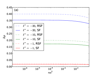
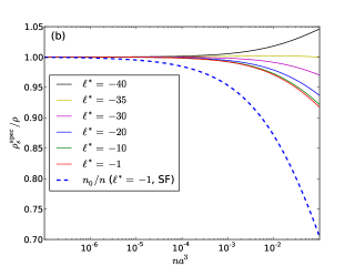
Figure 7: (Color online) Quantitative analysis of interaction effects at zero temperature: (a) raw $\Delta p$ signal; (b) spectroscopically determined superfluid fraction $\rho_{s}^{\rm spec}/\rho$, and comparison with the condensate fraction $n_{0}/n$. Note that the condensate depletion is significantly higher than the deviation of $\rho_{s}^{\rm spec}/\rho$ from 1. The curves are labelled from top to bottom.

Fig. 7 (a) shows the raw $\Delta p$ results for the relaxed ($\Delta p^{\mathrm{RSF}}$) and metastable ($\Delta p^{\mathrm{SF}}$) superfluids. Fig. 7 (b) shows the resulting spectroscopically determined superfluid fraction, from Eq. (41), using $na^{3}=10^{-7}$ to represent $na^{3}\approx 0$. For comparison, in Fig 7 (b) the dashed line shows the numerically determined condensate fraction $n_{0}/n$ for the SF footnote4 . The departure of the spectroscopic measurement of the superfluid fraction from $1$ [the solid lines in Fig. 7 (b)] shows that the error in determining the superfluid fraction by the spectroscopic method increases with interaction strength. However, this error is much smaller than the excited fraction $n_{\text{ex}}/n$. Therefore, the spectroscopic method allows one to distinguish clearly between the condensate fraction and the superfluid fraction in a strongly interacting BEC.

VI.3 Optimal experimental parameters

In the preceding sections we have shown that the spectroscopic method is capable of providing both a qualitative signature of superfluidity and a quantitatively accurate way to measure the superfluid fraction. We now turn to discuss the experimental parameters to use to optimise this technique as a quantitative measurement of superfluid fraction.

As was discussed in Section IV, there is a trade-off between the signal size and the quantitative accuracy of the method. In particular, we showed that it is advantageous to have as large a value of $\Delta\ell$ as possible, and then to increase $\Omega_{R}$ as much as possible to improve accuracy but not so much as to make the signal $\Delta p$ too small. From these considerations we were led to choose $\Delta\ell=50$ (from practical considerations of achieving beams of high angular momentum), and we settled on a compromise value of $\Omega_{R}=2\pi\times 100\,\mathrm{kHz}$. However, there still remains the question of what is the best detuning $\delta$ (and therefore value of $\ell^{*}$) to use. Formally, following Eq. (8) we should consider the limit $\ell^{*}\to 0$, such that the superfluid remains metastable even very close to $T_{c}$. But in this limit the signal becomes very small. What is a reasonable value of $\ell^{*}$ to use?

To explore this question, in Fig. 8 we present the results of calculations at zero temperature and $na^{3}=10^{-2}$, corresponding to a condensate depletion of about $12\%$.

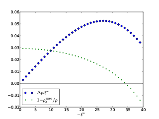
Figure 8: (Color online) Trade-off between signal size and accuracy at zero temperature. Signal size is assumed to be given by $\Delta p^{\prime}\ell^{*}$; compare Fig. 4 (c). Accuracy is determined by the deviation of the spectroscopic measurement (41) from the expected unity. This deviation has been calculated at $na^{3}=10^{-2}$ (corresponding to a condensate depletion $n_{\textrm{ex}}/n\approx 12\%$), amounting to a vertical slice through Fig. 7 (b) at $na^{3}=10^{-2}$.

In Fig. 8 the diamonds show the signal strength, as given by $\Delta p^{\prime}\ell^{*}$. This is the ideal difference between the signals of a normal fluid and a superfluid at $T=0$, neglecting higher-order corrections to $\Delta p_{\ell}$. As in Fig. 4 (c), this is a good approximation to the actual signal. These results show that, for the parameters chosen, the fractional imbalance $\Delta p$ must be measured to an accuracy of about $0.01$ to $0.05$. While this is a small fractional imbalance, it should be feasible to detect signals of this size by averaging over many shots.

The circles in Fig. 8 display the inaccuracy in the spectroscopic measurement of the superfluid fraction, i.e. the relative deviation of $\rho_{s}^{\rm spec}/\rho$ from the expected value of $1$ at $T=0$. Hence the circles in Fig. 8 correspond to a vertical slice through Fig. 7 (b) at $na^{3}=10^{-2}$. Here, an inaccuracy of $0.03$ means that a $100\%$ superfluid would be misinterpreted as only having $97\%$ superfluid fraction. In contrast, recall that the condensate fraction is about $88\%$. So this still allows a clear distinction between superfluid and condensate fraction.

The results in Fig. 8 would suggest picking $|\ell^{*}|\approx 35$, where the inaccuracy passes through zero. However, one should note that these results only show the inaccuracy at zero temperature. In Fig. 9 we plot the ratio $\rho^{\rm spec}_{s}/\rho_{s}$ as a function of temperature. Here $\rho_{s}^{\rm spec}$ is the spectroscopically measured superfluid density and $\rho_{s}$ is the expected superfluid density, as computed from the usual definition of superfluidity (1), $\rho_{s}/\rho=1-\langle\ell\rangle/\ell^{*}$.

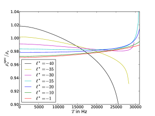
Figure 9: (Color online) Comparison of $\rho_{s}^{\rm spec}/\rho$ and $\rho_{s}/\rho=1-\langle\ell\rangle/\ell^{*}$ at $na^{3}=10^{-2}$ as a function of temperature (in terms of the ideal gas transition temperature $T_{c}\approx 31.1\,\mathrm{kHz}$). As in Fig. 6, the curves break off for $|\ell^{*}|>\ell^{*}_{\textrm{crit}}\simeq\sqrt{4\pi R^{2}an_{0}}$. The curves are labelled from top to bottom at the left-hand edge of the graph. Each curve starts at the $y$-value corresponding to the one in Fig. 7 (b) at $na^{3}=10^{-2}$.

The ratio stays close to one over a wide temperature range, showing that the spectroscopic method provides a good measure of the superfluid fraction.

Combining the issue of signal size and accuracy over a range of temperatures, we find that (for the parameters studied), a good choice is $|\ell^{*}|$ between $20$ and $30$. In this range, the signal size is $\simeq 0.05$; the spectroscopically measured superfluid fraction is accurate to about $0.02$ (much less than the depleted fraction of $0.12$); the accuracy remains at this level up to $\simeq 0.9T_{c}$.

VII Summary

In summary, we have assessed the feasibility of a recent proposal CooperHadzibabic2010 to measure the superfluid fraction of atomic BECs. This proposal involves the use of optically induced gauge fields to simulate rotation, and allows the superfluid response to appear in a spectroscopic signal. We have calculated the expected spectroscopic signatures for three-dimensional BECs with uniform density. One conclusion of our studies is the demonstration that this technique can be used to obtain a qualitative experimental signature of the superfluid response (by comparing the spectroscopic signals when the order of turning on the gauge field and cooling the gas is reversed), with a spectroscopic signal that is large enough to be detectable in experiment. Furthermore, and most importantly, we have shown that the technique can be used to extract a quantitative measurement of the superfluid density. The accuracy of the measurement technique can be improved at the expense of the size of the signal. Using realistic values for the experimental parameters, we have shown that a compromise can be reached where both (i) the signal is sufficiently large to be feasible to measure and (ii) the superfluid density is determined to sufficient accuracy to allow quantitatively useful information to be extracted. Notably, our results show that the technique can allow a clear experimental measurement of the distinction between condensate and superfluid fraction of a strongly interacting Bose gas. Our results support the usefulness of this technique CooperHadzibabic2010 for measuring the superfluid fraction, and provide guidance for the parameters required in future experimental implementations.

- (1) M. H. Anderson et al., Science 269, 198 (1995).
- (2) C. Raman et al., Phys. Rev. Lett. 83, 2502 (1999).
- (3) K. W. Madison, F. Chevy, W. Wohlleben, and J. Dalibard, Phys. Rev. Lett. 84, 806 (2000).
- (4) C. Ryu et al., Phys. Rev. Lett. 99, 260401 (2007).
- (5) I. Bloch, J. Dalibard, and W. Zwerger, Rev. Mod. Phys. 80, 885 (2008).
- (6) A. J. Leggett, Rev. Mod. Phys. 71, S318 (1999).
- (7) E. Andronikashvili, J. Phys. USSR 10, 201 (1946).
- (8) S. Riedl et al., ArXiv e-prints, arXiv:0907.3814v2 (2009).
- (9) T. Ho and Q. Zhou, Nature Physics 6, 131 (2009).
- (10) N. R. Cooper and Z. Hadzibabic, Phys. Rev. Lett. 104, 030401 (2010).
- (11) J. Dalibard, F. Gerbier, G. Juzeliūnas, and P. Öhberg, ArXiv e-prints, arXiv:1008.5378v1 (2010).
- (12) Bose-Einstein Condensation, edited by A. Griffin, D. W. Snoke, and S. Stringari (Cambridge University Press, Cambridge, 1996).
- (13) L. Tisza, Nature 141, 913 (1938).
- (14) L. Tisza, Phys. Rev. 72, 838 (1947).
- (15) L. D. Landau, J. Phys. USSR 5, 71 (1941).
- (16) S. Franke-Arnold, L. Allen, and M. Padgett, Laser & Photonics Reviews 2, 299 (2008).
- (17) J. M. Blatt and S. T. Butler, Phys. Rev. 100, 476 (1955).
- (18) F. Zambelli and S. Stringari, Phys. Rev. Lett. 81, 1754 (1998).
- (19) F. Chevy, K. W. Madison, and J. Dalibard, Phys. Rev. Lett. 85, 2223 (2000).
- (20) G. Juzeliūnas, P. Öhberg, J. Ruseckas, and A. Klein, Phys. Rev. A 71, 053614 (2005).
- (21) I. B. Spielman, Phys. Rev. A 79, 063613 (2009).
- (22) Y.-J. Lin et al., Phys. Rev. Lett. 102, 130401 (2009).
- (23) For simplicity, we neglect any quadratic Zeeman effect, assuming that the magnetic field is small.
- (24) For easy comparison with other parameters, for example the Rabi frequency, we express temperatures in frequency units, such that .
- (25) F. M. Fernndez, Introduction to perturbation theory in quantum mechanics (CRC Press, Boca Raton, FL, 2001).
- (26) Since we assumed that the condensate is in , the last term of in (30) refers to the condensate state; in general the argument to has to be changed appropriately: .
- (27) C. J. Pethick and H. Smith, Bose-Einstein Condensation in Dilute Gases; 2nd ed. (Cambridge University Press, Cambridge, 2008).
- (28) V. N. Popov, Functional Integrals and Collective Excitations (Cambridge University Press, Cambridge, 1988).
- (29) The condensate fraction deviates from the behaviour expected in an ideal Bose gas due to weak interactions as considered within the Popov approximation.
- (30) C. Chin, R. Grimm, P. Julienne, and E. Tiesinga, Rev. Mod. Phys. 82, 1225 (2010).
- (31) For the parameters used, this is indistinguishable from the condensate density determined by self-consistently solving Eq. (38) for , showing that non-parabolic corrections are irrelevant when considering the condensate fraction.