A Stable Explicit Scheme for Solving Inhomogeneous Constant Coefficients Differential Equation using Green’s Function

Abstract

A numerical explicit method to evaluates transient solutions of linear partial differential inhomogeneous equation with constant coefficients is proposed. A general form of the scheme for a specific linear inhomogeneous equation is shown. The method is applied to the wave equation and the diffuse equation and is investigated by simulating simple models. The numerical solutions of the proposed method show good agreement to the exact solutions. Comparing with explicit FDM, FDM shows the instability by the violation of CFL condition whereas the proposed method is always stable irrespective of any time step width.

1 Introduction

Many numerical method have been proposed to solve partial differential equations. Many of the proposed method is for spatial modeling. In spite of the variety of the spatial modeling, temporal modelings may not have been proposed so many.

As for the temporal modeling, when you solve a harmonic oscillating model in time, the time differentiation can be replace with $i\omega$. When you solve a transient model in time, the time differentiation is replaced with finite differentiation. The finite differentiation can be said to be the most popular method for the transient numerical solution.

The finite differentiation can be classified roughly into two categories. One is the explicit scheme and the rest is the implicit scheme [2]. The explicit scheme is easy to program and the amounts of computation for advancing one time step is smaller than the implicit method. One of the bad things is the time step width must be small enough to satisfy a condition otherwise numerical instability may occur. As for the implicit scheme, the computation is generally large for one time step but it is always stable for any time step width. From the user’s point of view the explicit method may be comfortable for programming.

In the meantime, Green’s functions are well used in theoretical physics but are not used in the numerical transient problems. This is because if you adopt Green’s function to solve a certain transient problem you have to integrate all over the history in time and space for each time step. Although the Green’s function may not be suitable for numerical simulation, the Green’s function is the response function of the basic equation against Dirac’s $\delta$ function or another functions. This means that the Green’s function gives the exact time variation of the system against a certain stimulation.

The reason of the instability of the explicit Finite Difference Method (FDM) is caused from the difficulty of the approximation of $\partial/\partial t$ with the several order of polynomials of $\Delta t$. There is no physical or mathematical inevitability for the approximation. Whereas the Green’s function is the exact solution of the basic equation so the time variation predicted by the Green’s function has the inevitability. It is a big motivation that the benefit of the Green’s function is to be integrated into the explicit time advancing to formulate a stable explicit scheme irrespective of any time step width.

The present paper describes a new scheme for transient solutions using Green’s function to solve inhomogeneous linear differential equation with constant coefficients. Although the scheme is a explicit scheme, it is always stable irrespective of any time step width different from the explicit FDM.

The preliminary works was applied to electromagnetics and diffuse equations [3][4][5]. In the present paper the general formulation of the scheme is described.

In the paper, generalized basic formulation is derived in section 2. Section 3 describes specific formulations for wave and diffuse equations. Numerical simulation using the proposed method is investigated in section 4 to show the effectiveness of the presented method. The numerical accuracy and stability is discussed in section 5.

2 Basic Formulation

Suppose a partial differential equation,

$${\cal D}_{t}u+{\cal D}_{x}u=S(x,t),$$ (1)

where ${\cal D}_{t},{\cal D}_{x}$ and $u$ are partial differential operator with respect to time $t$, space ${\bf x}=(x,y,z)$ and a certain physical value, respectively. The partial differential operators ${\cal D}_{t},{\cal D}_{x}$ are represented as,

$${\cal D}_{t} = \sum_{n}a_{n}\frac{\partial^{n}}{\partial t^{n}},$$ (2)

$${\cal D}_{x} = \sum_{l,m,n}b_{lmn}\frac{\partial^{l}}{\partial x^{l}}\frac{\partial^{m}}{\partial y^{m}}\frac{\partial^{n}}{\partial z^{n}},$$ (3)

where $a_{n},b_{lmn}$ are constant values. The authors are now interested in solving Eq.(1) to obtain the transient solution $u$ for the given source function $S({\bf x},t)$.

To solve the Eq.(1) by the proposed method, Fourier transformation is applied to the basic equation at first. A physical value can be expressed with integral form of Fourier components as,

$$A({\bf x},t)=\frac{1}{(2\pi)^{3/2}}\int_{-\infty}^{\infty}\tilde{A}({\bf k},t)e^{i{\bf k}{\bf x}}d{\bf k},$$ (4)

where ${\bf k}=(k_{x},k_{y},k_{z})$ is the wave number. Substituting Eq.(4) into Eq.(1) we have,

$${\cal D}_{t}\tilde{u}({\bf k},t)+{\cal K}\tilde{u}({\bf k},t)=\tilde{S}(k,t),$$ (5)

where

$${\cal K}=\sum_{l,m,n}b_{lmn}(ik_{x})^{l}(ik_{y})^{m}(ik_{z})^{n},$$ (6)

$\tilde{u}$ and $\tilde{S}$ is Fourier components with respect to $u$ and $S$, respectively.

Suppose a homogeneous equation relating Eq.(5),

$$({\cal D}_{t}+{\cal K})\tilde{u}({\bf k},t)={\cal L}(D)\tilde{u}({\bf k},t)=0,$$ (7)

where $D=d/dt$. The general solution of Eq.(7) is obtained as,

$$\tilde{u}({\bf k},t)=\sum_{j}\sum_{l=0}^{m-1}c_{lj}t^{l}e^{\lambda_{j}t},$$ (8)

where $m$ is the multiplicity of the solution $\lambda_{j}$, $\lambda_{j}$ is the solution of ${\cal L}(\lambda)=0$ which is the eigen equation of Eq.(7).

Let $m$ be 1, which means there is no multiplicity we have simplified general solution of Eq.(7).

$$\tilde{u}({\bf k},t)=\sum_{j}c_{j}e^{\lambda_{j}t}.$$ (9)

To obtain explicit scheme for the numerical solution of Eq.(5) we should have a recurrence formulation with respect to time step $t_{n}$. The explicit scheme is obtained directly from Eq.(9) as,

$$\tilde{u}({\bf k},t_{n}) = \sum_{j}c_{j}e^{\lambda_{j}t_{n}}$$

$$= \sum_{j}c_{j}e^{\lambda_{j}(t_{n-1}+\Delta t_{n})}$$

$$= \sum_{j}c_{j}e^{\lambda_{j}t_{n-1}}e^{\lambda_{j}\Delta t_{n}},$$

where

$$\Delta t_{n}=t_{n}-t_{n-1}.$$ (10)

Here the authors introduce a state variable $F_{n}^{j}$ for numerical formulation, which is defined as,

$$F_{n}^{j}=c_{j}e^{\lambda_{j}t_{n}}.$$ (11)

Then the authors have explicit scheme for the Eq.(7),

$$\tilde{u}({\bf k},t_{n}) = \sum_{j}F_{n}^{j},$$ (12)

$$= \sum_{j}F^{n-1}_{j}\cdot e^{\lambda_{j}\Delta t_{n}}.$$

General solution of Eq.(7) have been evaluated with a condition of no-multiplicity of the eigen values. The derived formulation is recursive with respect to time step. This means $\tilde{u}({\bf k},t_{n})$ can be obtained from the state variable of one time step before.

Now the authors consider the general solution of Eq.(7). The authors introduce an impulse function in order to obtain the general numerical solution of the inhomogeneous equation (5),

$$I(t,t_{n};\Delta t_{n})=\left\{\begin{array}[]{ll}0&(t\leq t_{n-1})\\ 1&(t_{n-1}<t<t_{n})\\ 0&(t_{n}\leq t)\end{array}\right..$$ (13)

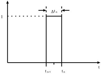
Figure 1: Impulse function for the Green’s function.

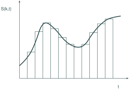
Figure 2: Approximation with the superposition of the Impulse functions.

Suppose the Green’s function $G_{n}(t)$ of Eq.(5) with respect to the impulse function which satisfies the equation;

$${\cal D}_{t}G_{n}(t)+{\cal K}G_{n}(t)=I(t;t_{n},\Delta t).$$ (14)

A certain source function $S({\bf k},t)$ can be approximated with superposition of the impulse functions as,

$$\tilde{S}({\bf k},t)\approx\sum_{n=0}^{N}\tilde{S}_{n}({\bf k},t_{n-1/2})I(t;t_{n},\Delta t),$$ (15)

where the time series $\tilde{S}_{n}({\bf k},t_{n-1/2})$ is given.

Equation (14) is a linear equation so a superposition of the solutions is also its solution. From Eqs.(15),(14) we obtain a superposed solution as,

$$\tilde{u}({\bf k},t)\approx\tilde{u}_{N}({\bf k},t)=\sum_{n=0}^{N}\tilde{S}_{n}({\bf k},t_{n})G_{n}(t),$$ (16)

where $t\geq t_{N}$.

The authors split summation in Eq.(16) into two parts to obtain an explicit scheme for the Eq.(5),

$$\tilde{u}_{N}({\bf k},t)=\sum_{n=0}^{N-1}\tilde{S}_{n}({\bf k},t_{n-1/2})G_{n}(t)+\tilde{S}_{N}({\bf k},t_{N-1/2})G_{N}(t).$$ (17)

If $t\geq t_{N}$, the first term of the right hand of the Eq.(17) is the solution of Eq.(7). So the first term can be described as,

$$\sum_{n=0}^{N-1}\tilde{S}_{n}({\bf k},t_{n-1/2})G_{n}(t) = \sum_{j}c_{j}e^{\lambda_{j}t},$$ (18)

$$= \sum_{j}F^{j}_{N-1}\cdot e^{\lambda_{j}(t-t_{N-1})}.$$

Now we have the explicit scheme to solve Eq.(5) with the proposed method in a general form.

$$\tilde{u}_{N}({\bf k},t)=\sum_{j}F^{j}_{N-1}\cdot e^{\lambda_{j}(t-t_{n-1})}+\tilde{S}_{N}({\bf k},t_{N-1/2})G_{N}(t).$$ (19)

In the following section we will investigate two concrete examples using the proposed scheme.

3 Formulation Examples

We present two examples of the proposed formulation for solving partial differential equations which is derived in the present section. First one is a wave equation and second is a diffuse equation. They both have constant coefficients.

3.1 Wave Equation

Here we consider a wave equation of constant coefficients.

$$\frac{1}{c^{2}}\frac{\partial^{2}u({\bf x},t)}{\partial t^{2}}-\nabla^{2}u({\bf x},t)=S({\bf x},t),$$ (20)

where $u$ is a physical value, ${\bf x}$ and $t$ are the coordinates in space and time respectively, $c$ is the speed of the wave propagation. $S$ is a source function and is given. We shows the formulation procedure of Eq.(20) in the following.

Applying Fourier transform to Eq.(20) gives,

$$\frac{1}{c^{2}}\frac{\partial^{2}\tilde{u}({\bf k},t)}{\partial t^{2}}+k^{2}\tilde{u}({\bf k},t)=\tilde{S}({\bf k},t),$$ (21)

where $k^{2}=k_{x}^{2}+k_{y}^{2}+k_{z}^{2}$. Now we have an ordinary differential equation instead of partial differential equation.

Consider the Green’s function of Eq.(21) against the impulse function (Eq.(13)), we have an equation,

$$\frac{1}{c^{2}}\frac{\partial^{2}G_{n}(t)}{\partial t^{2}}+k^{2}G_{n}(t)=I(t,t_{n};\Delta t_{n}).$$ (22)

Then the eigen equation can be obtained as,

$$L(\lambda)=(\lambda^{2}+(kc)^{2})=0,$$ (23)

so we have the eigen solutions.

$$\lambda=\pm ikc.$$ (24)

According to Eq.(19) the solution can be described as,

$$\tilde{u}_{N}({\bf k},t) = F^{+}_{N-1}\cdot e^{ikc(t-t_{N-1})}+F^{-}_{N-1}\cdot e^{-ikc(t-t_{N-1})}$$ (25)

$$+\tilde{S}_{N}({\bf k},t_{N})G_{N}(t),$$

where $F_{N}^{+}$ and $F_{N}^{-}$ are the state variables for $\lambda=ikc$ and $\lambda=-ikc$, respectively.

Equation (22) can be solved analytically as,

$$G_{N}(t) = -i\frac{\sin(kc\Delta t_{N}/2)}{k^{2}}\left[e^{ikc(t-t_{N}+\Delta t_{N}/2)}-e^{-ikc(t-t_{N}+\Delta t_{N}/2)}\right],$$

$$(t\geq t_{N}).$$

Equation (3.1) is the Green’s function which satisfies Eq.(22).

We redefine the state variable $F_{N}$ as,

$$F^{\pm}_{N}=F^{\pm}_{N-1}\cdot e^{\pm ikc\Delta t_{N}}+\tilde{S}(k,t_{N-1/2})e^{\pm ikc\Delta t_{N}/2}\sin\frac{kc\Delta t_{N}}{2}.$$ (27)

Then we have the formulation by the proposed scheme.

$$\tilde{u}(k,t)=-\frac{i}{k^{2}}\left[e^{ikc(t-t_{N})}F^{+}_{N}-e^{-ikc(t-t_{N})}F^{-}_{N}\right]\hskip 14.22636pt(t\geq t_{N}).$$ (28)

3.2 Diffuse Equation

Suppose a diffuse equation with constant diffusion coefficient as,

$$\frac{\partial u({\bf x},t)}{\partial t}-c\nabla^{2}u({\bf x},t)=S({\bf x},t),$$ (29)

where $c$ is the diffusion coefficient, $u({\bf x},t)$ and $S({\bf x},t)$ are functions of space ${\bf x}$ and time $t$. Applying Fourier transformation to the Eq.(29) to get the Fourier transformed equation.

$$\frac{\partial\tilde{u}({\bf k},t)}{\partial t}+ck^{2}\tilde{u}({\bf k},t)=\tilde{S}({\bf k},t).$$ (30)

Same as the procedure deriving the formulation for the wave equation we have an equation to consider as,

$$\frac{\partial G_{n}(t)}{\partial t}+ck^{2}G_{n}(t)=I(t,t_{n};\Delta t).$$ (31)

Equation (31) can be solved analytically and then we have,

$$G_{N}(t)=\Delta t_{N}\frac{\sinh ck^{2}\Delta t_{N}/2}{ck^{2}\Delta t_{N}/2}e^{-ck^{2}(t-t_{N}+\Delta t_{N}/2)}.$$ (32)

Same as the formulation of the wave equation we have the explicit form of the solution as,

$$\tilde{u}_{N}({\bf k},t)=F^{N}({\bf k},t_{N})e^{-ck^{2}(t-t_{N})},$$ (33)

where

$$F^{N}({\bf k}) = F^{N-1}({\bf k})e^{-ck^{2}\Delta t_{N}}$$

$$+ \Delta t\frac{\sinh ck^{2}\Delta t_{N}/2}{ck^{2}\Delta t_{N}/2}e^{-ck^{2}\Delta t_{N}/2}\tilde{S}({\bf k},t_{N-1/2}).$$

In the next section we will verify the effectiveness of the obtained formulations by applying to a simple one dimensional problems.

4 Numerical Experiments

A numerical experiments by the proposed scheme are shown here. For reader’s understanding simple one dimensional examples are shown but the scheme can be applied to multi-dimension straightforwardly.

The source term is given and the same source function is used for both examples. The source function adopted here is a Gaussian distribution in space and sinusoidal in time.

$$S(x,t)=\left\{\begin{array}[]{ll}0&(t<0)\\ e^{-\frac{({\bf x}-{\bf x}_{0})^{2}}{2\Delta x^{2}}}\sin\omega_{0}t&(t\geq 0)\end{array}\right.,$$ (34)

where $x_{0},\Delta x$ are the centre and the half-value width of the Gaussian distribution, respectively.

The Fourier transformed Gaussian function $\tilde{S}({\bf k})$ is analytically evaluated as,

$$\tilde{S}(k)=(2\pi\Delta x^{2})^{1/2}e^{-k^{2}\Delta x^{2}/2}e^{-i{\bf k}{\bf x}_{0}}.$$ (35)

Figure 3(a) and 3(b) shows the distribution of the function in space and time, respectively. The common data in both wave and diffuse equations is shown in Table 1.

Table 1: Common Parameters for the Simulation

Grid Number	Length of the system	Grid Width $\Delta x$
64	10.0	10.0/63

(a) Spatial distribution of the source function.

(b) Temporal variation of the source function.

Figure 3: The source function.

The proposed method is denoted as transient Green method (hereafter TGM) for convenience.

4.1 Wave Equation

A simple one dimensional numerical simulation is performed in order to investigate the characteristics of the TGM. The basic equation to solve is Eq. (21) and finite difference solution is also calculated for comparison.

The analytical solution of the basic equation can be obtained and we have,

$$\tilde{u}_{E}(k,t)=\frac{e^{-k^{2}\delta_{x}^{2}/2-ikx_{0}}}{\omega_{0}^{2}-(ck)^{2}}\left[\frac{\omega}{ck}\sin ckt-\sin\omega_{0}t\right].$$ (36)

The particular parameters for the wave equation is listed in Table 2.

Table 2: Parameters for wave equation.

Wave Speed ($c$)	Time Step Width $\Delta t$	Frequency ($\omega/2\pi$)
1.0	0.01	3.14159

Figure 4: Snapshot of $u_{N}({\bf x},t)$ and $u_{E}({\bf x},t)$ at $t=1.0$.

The snapshot at $t=1.0$ is shown in Fig.4. Although time advancing is performed in ${\bf k}$ space, the figure shows the real space distribution by inverse Fourier transformation to help the reader’s understanding. Fast Fourier Transform is used to calculate. The result shows the good agreement with TGM and exact solution.

Figure 5: Standard deviation of TGM and FDM from the exact solution as a function of $\Delta t$.

Figure 5 shows the standard deviation from the exact solutions in ${\bf k}$ space as a function of time step width ($\Delta t$).

$$Er(t;\Delta t)=\sqrt{\sum_{k}(u({\bf k},t;\Delta t)-u_{E}({\bf k},t))^{2}}.$$ (37)

In Fig.5 the FDM and TGM show error with ${\cal O}(\Delta t^{2})$. When the time step width $\Delta t$ becomes big enough to violate the CFL condition the result of FDM shows the numerical instability. While TGM doesn’t show any numerical instability. It seems to be always stable irrespective of any time step width.

4.2 Diffuse Equation

Same as Sec. 4.1, numerical simulation is performed with TGM and FDM for solving a simple one dimensional diffuse equation problem. The equation to solve is a diffuse equation (Eq.(30)). The analytical exact solution is obtained for this equation, which is:

$$\tilde{u}_{E}(k,t) = \frac{e^{-k^{2}\delta_{x}^{2}/2-ikx_{0}}}{(ck^{2})^{2}+\omega_{0}^{2}}$$

$$\times \left[\omega_{0}e^{-ck^{2}t}+ck^{2}\sin\omega_{0}t-\omega_{0}\cos\omega_{0}t\right].$$

The particular parameters adopted in the experiment is listed in Table 3.

Table 3: Parameters particularly used for Diffuse Equation.

Diffuse Coeff. ($c$)	Time Step Width $\Delta t$	Frequency ($\omega/2\pi$)
3.0	0.001	20.0

The snapshot at $t=0.1$ is shown in Fig.6. The solution computed by TGM and exact solution indicate good agreement.

Figure 6: Snapshot of $u_{N}({\bf x},t)$ and $u_{E}({\bf x},t)$ at $t=0.1$.

The errors of the TGM and the FDM are shown in Fig.7. The error is evaluated form Eq.(37) same as the case of wave equation.

Figure 7: Standard deviation of TGM and FDM from the exact solution as a function of $\Delta t$.

Figure 7 shows numerical instability is occurred with the violation of CFL condition whereas the results of the TGM doesn’t show any numerical instability irrespective of any time step width.

The FDM is the Euler’s scheme so the error is ${\cal O}(\Delta t)$. According to the Fig.7, TGM has accuracy of ${\cal O}(\Delta t^{2})$.

5 Discussion

5.1 Numerical Accuracy

The numerical error of the proposed scheme potentially contains the discretization errors in time and space.

The spatial accuracy of TGM is determined by the Fourier transformation. If the Fast Fourier Transformation is adopted the data can be transformed exactly. This means the transformed data contains no truncation error essentially.

The temporal accuracy of the proposed method depend upon the accuracy of the integration method of the source term $S({\bf k},t)$. In the presented scheme here (Eqs.(28),(33)) rectangle mid-point rule is adopted for time integration (Eq.(15)). So discretization error of Eqs.(28),(33) is ${\cal O}(\Delta t^{2})$. If you adopt more accurate integration scheme the accuracy of the proposed scheme also becomes more accurate.

5.2 Numerical Stability

The numerical stability of the proposed method is discussed in the section.

As for the finite difference method the explicit scheme is unstable unless the time step width $\Delta t$ is small enough to satisfy a condition. The criteria is well known as Courant Friedrichs and Lewy (CFL) condition. For instance CFL condition of the simple explicit scheme for diffuse equation (29) is;

$$\Delta t<\frac{2\Delta x^{2}}{c}.$$

If the condition is violated the simulation result may be far from the exact solution which you want to obtain. The unstableness comes from the difficulty in approximating the solution with first or second order polynomials. While the proposed method is derived from the superposition of the Green’s function which are analytical solutions.

Now we consider the numerical stability of the TGM solution for Eq.(7). The TGM formulation is given by Eq.(12). The general solution of Eq.(7) is already given by Eq.(9). The state variable $F_{n}^{j}$ also given by Eq.(11).

When $F^{j}_{n-1}$ satisfy the equation:

$$F^{j}_{n-1}=c_{j}e^{\lambda_{j}t_{n-1}}.$$

The $F^{j}_{n}$ can be in TGM formulation as,

$$F^{j}_{n} = F^{j}_{n-1}\cdot e^{\lambda_{j}\Delta t_{n}},$$

$$= c_{j}e^{\lambda_{j}t_{n-1}}\cdot e^{\lambda_{j}\Delta t_{n}},$$

$$= c_{j}e^{\lambda_{j}t_{n}}.$$

So we find the TGM solution is exactly identical with the analytical solution. This is always true irrespective of any time step width $\Delta t$. This result indicates the TGM formulation is always stable with any time step width as is shown in section 4

6 Conclusion

A numerical method to compute explicitly for transient solution of linear partial differential inhomogeneous equation with constant coefficients is proposed. It is shown that the proposed method gives the transient solution from the state variables at the one time step before explicitly and always numerically stable irrespective of any time step width.

References

- [1] R. Courant, K.O. Friedrichs, and H. Lewy, Math. Ann., 100, 1928, 32.
- [2] D.A. Anderson, J.C.Tannehill, and R.H.Pletcher, Computational Fluid Mechanics and Heat Transfer, McGraw-Hill, 1984, p108.
- [3] Hiroshi Abe, Transaction on Information Processing Society of Japan, 1992, p.1006.
- [4] Hiroshi Abe, Digests of the Fifth Biennial IEEE Conference on Electromagnetic Field Computation, Harvey Mudd College, Claremont, CA, USA, 1992, MP39.
- [5] Hiroshi Abe, Annual Meeting of Japan Society of Industry and Applied Mathematics, 1993.