Escape Process and Stochastic Resonance Under Noise Intensity Fluctuation

Abstract

We study the effects of noise-intensity fluctuations on the stationary and dynamical properties of an overdamped Langevin model with a bistable potential and external periodical driving force. We calculated the stationary distributions, mean-first passage time (MFPT) and the spectral amplification factor using a complete set expansion (CSE) technique. We found resonant activation (RA) and stochastic resonance (SR) phenomena in the system under investigation. Moreover, the strength of RA and SR phenomena exhibit non-monotonic behavior and their trade-off relation as a function of the squared variation coefficient of the noise-intensity process. The reliability of CSE is verified with Monte Carlo simulations.

I Introduction

Langevin models have become increasingly important in modeling systems subject to fluctuations. These models have a wide range of applications in physics, chemistry, electronics, biology, and financial market analysis. In many applications, fluctuations are modeled in terms of white noise, which has a delta function correlation with constant noise intensity. In general, fluctuations are space-time dependent phenomena; hence, the noise intensity fluctuates temporally and/or spatially. Nevertheless, white noise has been be used to model fluctuations because at the typical level of physical description, variations in noise intensity can be ignored. However, if the variation in the noise intensity fluctuations is large and if it occurs in time scales comparable to the physical description of interest, the effects of such fluctuations have to be taken into account. Noise intensity fluctuations due to environmental variations are particularly important in biological applications. For instance, the stochasticity of a gene expression mechanism is derived from intrinsic (discreteness of particle number) and extrinsic (noise sources external to the system) fluctuations. Because extrinsic fluctuations are subject to biological rhythms with different time scales Novak:2008:BiochemOsc , their noise intensity varies temporally.

In financial market analysis, stochastic volatility models (e.g., the Hull & White model and Heston model) incorporate temporal noise intensity fluctuations Hull:1987:SV ; Heston:1993:Volatility ; Dragulescu:2002:Heston ; Andersson:2003:SV . The stochastic volatility models assume that noise variance is governed by stochastic processes. In physics, superstatistics Wilk:2000:NEXTParam ; Beck:2001:DynamicalNEXT ; Beck:2003:Superstatistics ; Beck:2006:SS_Brownian ; Beck:2009:RecentSS ; Beck:2010:GStatMech take spatial and/or temporal environmental fluctuations into account. Superstatistics has been applied to stochastic processes, and it has introduced noise intensity fluctuations Beck:2001:DynamicalNEXT ; Beck:2006:SS_Brownian ; Jizba:2008:SuposPD ; Queiros:2008:SSMultiplicative ; Hasegawa:2010:qExpBistable ; Rodriguez:2007:SS_Brownian ; Straeten:2010:SkewedSS , by calculating stationary distributions in a Bayesian manner. A previous study Queiros:2005:VolatilityNEXT indicates the similarity between distributions of a stochastic volatility model and Tsallis statistics, which has the same stationary distribution ($q$-Gaussian distribution) as superstatistics in specific cases.

Most discussions on stochastic volatility models are limited to linear drift terms; hence, the application of such models to physical, chemical, or biological systems, accompanied by nontrivial drift terms and multiplicative noise, is nontrivial. In our previous paper Hasegawa:2010:SIN , we proposed an approximation scheme that can be applied to general drift terms. We considered Langevin equations where the white Gaussian noise intensity is governed by the Ornstein–Uhlenbeck process:

$$\frac{dx}{dt} = f(x)+s\xi_{x}(t),$$ (1)

$$\frac{ds}{dt} = -\gamma(s-\alpha)+\sqrt{\gamma}\xi_{s}(t),$$ (2)

where $f(x)$ is a drift term ($f(x)=-\partial_{x}U(x)$, where $U(x)$ is a potential), $\gamma$ is the relaxation rate, and $\xi_{x}(t)$, $\xi_{s}(t)$ denote white Gaussian noise with the correlation [$\left\langle\xi_{x}(t)\xi_{x}(t^{\prime})\right\rangle=2D_{x}\delta(t-t^{\prime})$ and $\left\langle\xi_{s}(t)\xi_{s}(t^{\prime})\right\rangle=2D_{s}\delta(t-t^{\prime})$]. In the present paper, we call the term $s\xi_{x}(t)$ the stochastic intensity noise (SIN) because the noise intensity is governed by a stochastic process. In Ref. Hasegawa:2010:SIN , we obtained a time evolution equation using adiabatic elimination with an eigenfunction expansion Kaneko:1976:AdiabaticElim . Although the previously developed method Hasegawa:2010:SIN can be applied to nonlinear drift terms, its application is limited to $\gamma\gg 1$ [$\gamma$ is the relaxation rate in Eq. (2)]. At the same time, we showed that the time evolution equation of $P(x;t)$ is a higher order Fokker–Planck equation (FPE) having derivatives of orders higher than two Hasegawa:2010:SIN . Analytic calculations of dynamical quantities such as mean-first passage time (MFPT) and stochastic resonance (SR) are mainly developed for one-variable FPEs; hence, their use in higher-order FPEs is nontrivial. Accordingly, in this paper, we investigate the dynamical properties of the coupled equations (1) and (2), expanding functions of interest (stationary distributions and eigenfunctions) in terms of an orthonormal complete set. This technique is extensively used to solve FPEs numerically (e.g., the matrix continued fraction method. For details, please see Ref. Risken:1989:FPEBook and the references therein). Complete set expansion (CSE) can be applied to polynomial drift terms, and it can, in principle, solve for the entire range of $\gamma$; on the other hand, the adiabatic elimination based method is limited to $\gamma\gg 1$ Hasegawa:2010:SIN .

In the present paper, we investigate MFPT and SR with a bistable potential [see Eq. (3)]. As stated above, SIN is particularly important in biological mechanisms. In a zeroth-order approximation, many important biological mechanisms, such as neuron and gene expression, can be modeled with a bistable potential. MFPT and SR have also been extensively investigated in such biological mechanisms. In the calculation of MFPT, we show that MFPT, as a function of $\gamma$, has a minimum around $\gamma\simeq 1$, which is equivalent to resonant activation (RA) Doering:1992:ResonantActivation ; Zurcher:1993:ResoAct ; Marchi:1996:ResoAct ; Boguna:1998:RAproperties ; Mantegna:2000:ExpRA ; Fiasconaro:2011:AsymRA . Furthermore, by changing $\rho$ (the squared variation coefficient of noise intensity fluctuations [see Eq. (11)]), MFPT also has a minimum around $\rho\simeq 1$. In the calculation of SR, we show that the SR effect is smaller for smaller $\gamma$, which indicates that the SR effect is maximized under white noise. In addition, the spectral amplification factor, as a function of $\rho$, has a minimum around $\rho\simeq 1$. These results show that the strength of RA and SR effects cannot be maximized simultaneously. All the calculations are performed using CSE, whose reliability is evaluated via Monte Carlo (MC) simulations.

The remainder of this paper is organized as follows. In Sec. II, we describe the model adopted in this study. In Sec. III, stationary distributions are calculated using CSE. In Sec. IV, we calculate MFPT, which is approximated by the smallest non-vanishing eigenvalue. In Sec. V, we investigate the spectral amplification factor of SR by using the linear response approximation. In Sec. VI, we discuss the effects of noise intensity fluctuations on RA and SR. Finally, in Sec. VII, we conclude the paper.

II The Model

We consider the Langevin equations given by Eqs. (1) and (2) with the bistable potential

$$U(x)=\frac{x^{4}}{4}-\frac{x^{2}}{2},$$ (3)

i.e., $f(x)=x-x^{3}$. In this paper, we investigate the $\gamma>0$ case for Eq. (2) because $s(t)$ is constant ($s(t)=s(0)$) for $\gamma=0$, and the resulting SIN is equivalent to conventional white Gaussian noise.

By interpreting Eqs. (1) and (2) in the Stratonovich sense, a probability density function $P(x,s;t)$ of $(x,s)$ at time $t$ is governed by the FPE:

$$\frac{\partial}{\partial t}P(x,s;t)=\mathscr{L}_{0}P(x,s;t),$$ (4)

where $\mathscr{L}_{0}$ is an FPE operator defined as

$$\mathscr{L}_{0}=\mathscr{L}_{x}+\gamma\mathscr{L}_{s},$$ (5)

with

$$\mathscr{L}_{x}=-\frac{\partial}{\partial x}f(x)+s^{2}D_{x}\frac{\partial^{2}}{\partial x^{2}},$$ (6)

$$\mathscr{L}_{s}=\frac{\partial}{\partial s}(s-\alpha)+D_{s}\frac{\partial^{2}}{\partial s^{2}}.$$ (7)

For the asymptotic case $\gamma\rightarrow\infty$, we used the adiabatic elimination technique to obtain the FPE operator Hasegawa:2010:SIN

$$\mathscr{L}_{0}=-\frac{\partial}{\partial x}f(x)+Q\frac{\partial^{2}}{\partial x^{2}}\hskip 10.00002pt(\mathrm{for}\,\,\,\,\gamma\rightarrow\infty),$$ (8)

where $Q$ is the effective noise intensity given by

$$Q=D_{x}(D_{s}+\alpha^{2}).$$ (9)

Equation (9) is in agreement with the noise intensity of the correlation function, i.e., $\left\langle s(t)\xi_{x}(t)s(t^{\prime})\xi_{x}(t^{\prime})\right\rangle=2Q\delta(t-t^{\prime})$ (see the Appendix).

From Eq. (7), the stationary distribution $P_{st}(s)$ of the intensity-modulating term $s$ is given by

$$P_{st}(s)=\frac{1}{\sqrt{2\pi D_{s}}}\exp\left\{-\frac{1}{2D_{s}}(s-\alpha)^{2}\right\}.$$ (10)

Here, we introduce the squared variation coefficient of the noise intensity fluctuation for later use. The squared variation coefficient $\rho$ is defined as

$$\rho=\frac{D_{s}}{\alpha^{2}},$$ (11)

where $\rho$ denotes the squared ratio between the standard deviation and mean of Eq. (10), similar to the Fano factor. Figure 1 shows some trajectories of SIN with (a) $\rho=0.01$, (b) $\rho=0.1$, (c) $\rho=1$, and (d) $\rho=100$. These trajectories have the same effective noise intensity $Q$. As $\rho\rightarrow 0$, SIN reduces to white Gaussian noise with noise intensity $Q=D_{x}\alpha^{2}$.

In the present paper, the FPE of Eq. (4) is solved using CSE and MC. MC is performed by adopting the Euler forward method with time resolution $\Delta t=10^{-4}$ (for details of the method, see Ref. Risken:1989:FPEBook ).

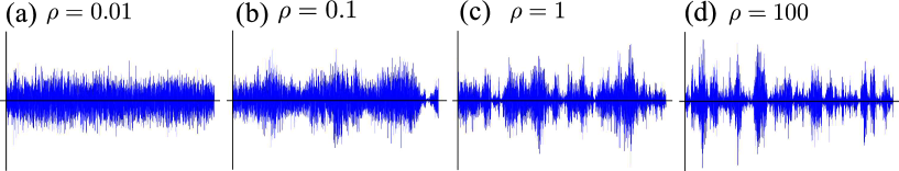
Figure 1: (Color online) Trajectories of SIN for four parameter values of $\rho$ (squared variation coefficient): (a) $\rho=0.01$, (b) $\rho=0.1$, (c) $\rho=1$, and (d) $\rho=100$. We varied $\rho$ while keeping the effective intensity $Q$ constant.

III Stationary Distributions

We calculate the stationary distributions of the coupled Langevin equations (1) and (2), which have been discussed previously Hasegawa:2010:SIN for $\gamma\gg 1$. The method adopted in this paper is different from the previous one Hasegawa:2010:SIN in the range of $\gamma$ (previously Hasegawa:2010:SIN , it was limited to $\gamma\gg 1$). In the following, we first investigate the effects of noise intensity fluctuations on the stationary distributions. Then, the calculations of the stationary distributions are used for the spectral amplification factor in SR (Sec. V).

The stationary distribution $P_{0}(x,s)$ of $(x,s)$ has to satisfy the differential equation:

$$\mathscr{L}_{0}P_{0}(x,s)=0,$$ (12)

where $\mathscr{L}_{0}$ is an FPE operator defined in Eq. (4). In order to solve Eq. (12), we employ CSE, which expands $P_{0}(x,s)$ in terms of an orthonormal complete set. This technique is extensively used in stochastic processes (e.g., the matrix continued fraction method Risken:1989:FPEBook ). CSE can handle systems with polynomial drift terms and it can, in principle, handle the entire range of $\gamma$. However, in practical calculations, we are restricted to $\gamma\geq 0.3$ because of numerical instability. Considering the symmetry $x\rightarrow-x$ in $\mathscr{L}_{0}$ and the relation $\varphi_{2k}(-x)=\varphi_{2k}(x)$, the stationary distribution $P_{0}(x,s)$ admits the even parity expansion:

$$P_{0}(x,s)=\varphi_{0}(x)\psi_{0}(s)\sum_{k=0}^{K}\sum_{\ell=0}^{L}C_{k,\ell}\varphi_{2k}(x)\psi_{\ell}(s),$$ (13)

with

$$\varphi_{k}(x)=\sqrt{\frac{\zeta}{2^{k}k!\sqrt{\pi}}}H_{k}(\zeta x)\exp\left(-\frac{1}{2}\zeta^{2}x^{2}\right),$$ (14)

$$\psi_{\ell}(s)=\left(\frac{1}{2\pi D_{s}}\right)^{1/4}\sqrt{\frac{1}{2^{\ell}\ell!}}H_{\ell}\left(\eta\right)\exp\left(-\frac{1}{2}\eta^{2}\right).$$ (15)

Here, $C_{k,\ell}$ are expansion coefficients, $\eta=\sqrt{1/(2D_{s})}(s-\alpha)$, $H_{n}(z)$ is the $n$th Hermite polynomial, and $\zeta$ is a (positive) scaling parameter that affects the convergence of CSE. $K$ and $L$ are truncation numbers which provide the precision of the obtained solutions. The orthonormality and complete relations read

$$\int dx\,\varphi_{k^{\prime}}(x)\varphi_{k}(x)=\delta_{k^{\prime},k},\hskip 10.00002pt\int ds\,\psi_{\ell^{\prime}}(s)\psi_{\ell}(s)=\delta_{\ell^{\prime},\ell},$$ (16)

where $\delta_{k^{\prime},k}$ is Kronecker’s delta function. The term $\psi_{0}(s)\psi_{\ell}(s)$ forms eigenfunctions of $\mathscr{L}_{s}$ [Eq. (7)], i.e.,

$$\mathscr{L}_{s}\left[\psi_{0}(s)\psi_{\ell}(s)\right]=-\ell\psi_{0}(s)\psi_{\ell}(s).$$ (17)

After multiplying $\varphi_{2k^{\prime}}(x)\psi_{\ell^{\prime}}(s)/(\varphi_{0}(x)\psi_{0}(s))$ by Eq. (12) and integrating with respect to $x$ and $s$, we obtain the following linear algebraic equation:

$$0 = C_{k,\ell}\left(2k-\frac{6k^{2}}{\zeta^{2}}-\gamma\ell\right)$$ (18)

$$+C_{k-1,\ell}\sqrt{2k(2k-1)}\left[1-\frac{3}{2\zeta^{2}}(2k-1)+2\zeta^{2}D_{x}\left\{\alpha^{2}+2D_{s}\left(\ell+\frac{1}{2}\right)\right\}\right]$$

$$-C_{k+1,\ell}\frac{k}{\zeta^{2}}\sqrt{(2k+1)(2k+2)}-C_{k-2,\ell}\frac{1}{2\zeta^{2}}\sqrt{2k(2k-1)(2k-2)(2k-3)}$$

$$+2C_{k-1,\ell+2}\zeta^{2}D_{x}D_{s}\sqrt{2k(2k-1)(\ell+2)(\ell+1)}+2C_{k-1,\ell-2}\zeta^{2}D_{x}D_{s}\sqrt{2k(2k-1)\ell(\ell-1)}$$

$$+4C_{k-1,\ell-1}\zeta^{2}\alpha D_{x}\sqrt{2D_{s}k(2k-1)\ell}+4C_{k-1,\ell+1}\zeta^{2}\alpha D_{x}\sqrt{2D_{s}k(2k-1)(\ell+1)}.$$

Because all coefficients vanish for $(k,\ell)=(0,0)$, $C_{0,0}$ can be determined by a normalization condition [$\int ds\int dx\,P_{0}(x,s)=1$] as $C_{0,0}=1$. The two-dimensional coefficients $C_{k,\ell}$ can be cast in the form of one-dimensional coefficients $\mathcal{C}_{m}$ by the following one-to-one mapping Denisov:2009:ACmotorFPE :

$$m=1+(1+L)k+\ell.$$ (19)

By using Eq. (19), $C_{k,\ell}$ can be transformed into $\mathcal{C}_{m}$ with $1\leq m\leq M$, where $M=(1+K)(1+L)$. Eq. (18) can be solved using general linear algebraic solvers. CSE transforms the differential equations into linear algebraic equations, which are easier to solve. From Eq. (8), the stationary distribution $P_{0}(x)$ of $x$ in the asymptotic case $\gamma\rightarrow\infty$ is given by

$$P_{0}(x)=\int ds\,P_{0}(x,s)=\frac{1}{Z}\exp\left(-\frac{U(x)}{Q}\right)\hskip 10.00002pt(\mathrm{for}\,\,\,\gamma\rightarrow\infty),$$ (20)

where $Z$ is a normalizing constant.

In calculating stationary distributions using CSE, we have to determine $K$, $L$, and $\zeta$. We increase $K$ and $L$ until the stationary distributions converge. Although larger values of $K$ and $L$ allow better approximation, we find that using excessively large values numerically gives rise to divergent distributions. Fig. 2 shows stationary distributions with different parameters: $D_{x}=1$, $D_{s}=0.1$, and $\alpha=0.1$ (Fig. 2(a)); and $D_{x}=1$, $D_{s}=1$, and $\alpha=0.5$ (Fig. 2(b)). Figs. 2(a) and (b) show stationary distributions calculated using CSE for four $\gamma$ values: $\gamma=0.3$ (solid line), $\gamma=1$ (dotted line), $\gamma=10$ (dot-dashed line), and $\gamma\rightarrow\infty$ (dot-dot-dashed line). Although the CSE method is valid, in principle, for the entire range of $\gamma$, it appears that small values of $\gamma$ give rise to numerical instability. Consequently, the smallest value used in this paper is $\gamma=0.3$. For $\gamma\rightarrow\infty$, we used the asymptotic expression given by Eq. (20). The stationary distributions of MC simulations were computed for four $\gamma$ values: $\gamma=0.3$ (circles), $\gamma=1$ (squares), $\gamma=10$ (triangles), and $\gamma=100$ (crosses). Total $10^{6}$ samples each were calculated for the empirical probability densities. Higher peaks emerge at metastable sites for smaller $\gamma$. The CSE stationary distribution of $\gamma\rightarrow\infty$ and the MC stationary distribution of $\gamma=100$ are very close, which supports the result that a system driven by SIN reduces to one driven by white Gaussian noise with effective noise intensity $Q$.

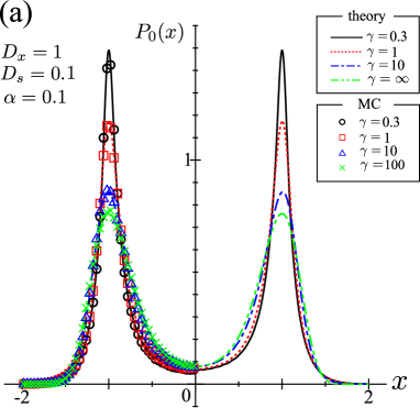
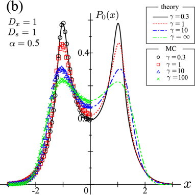
Figure 2: (Color online) Stationary distributions for systems driven by additive SIN. The lines and symbols represent distributions calculated using CSE and MC methods, respectively. The parameters are (a) $D_{x}=1$, $D_{s}=0.1$, $\alpha=0.1$ and (b) $D_{x}=1$, $D_{s}=1$, $\alpha=0.5$, with $\gamma=0.3$ (solid lines and circles), $1$ (dotted lines and squares), and $10$ (dot-dashed lines and triangles). Furthermore, the dot-dot-dashed lines are given by Eq. (20), which corresponds to $\gamma\rightarrow\infty$, and the crosses denote MC results with $\gamma=100$. For viewability, MC data are plotted only for $x<0$.

IV Mean First Passage Time

In order to study the dynamical properties of systems driven by SIN, we calculate MFPT. With regard to the stochastic volatility model, an escape problem was investigated for the extended Heston volatility model in a cubic potential using MC simulations Bonanno:2007:EscapeSV . Non-monotonic phenomena such as noise-enhanced stability (NES) Mantegna:1996:NES ; Spagnolo:2008:NES_review ; Dubkov:2004:NES ; Fiasconaro:2009:NESinColoredNoise were reported for this model. Another study Iwaniszewski:2008:RAtemperature considered a Langevin system, where the temperature (i.e., noise intensity) takes two values in a random dichotomatic manner, indicating the occurrence of an RA Doering:1992:ResonantActivation ; Zurcher:1993:ResoAct ; Marchi:1996:ResoAct ; Boguna:1998:RAproperties ; Mantegna:2000:ExpRA ; Fiasconaro:2011:AsymRA phenomenon.

First, we investigate two basins of attractors and a separatix that separates them in $(x,s)$ space. Without fluctuations, the deterministic dynamics of Eqs. (1) and (2) are given by

$$\frac{dx}{dt}=f(x),\hskip 10.00002pt\frac{ds}{dt}=-\gamma(s-\alpha).$$ (21)

Considering the quartic bistable potential $f(x)=x-x^{3}$, Eq. (21) has three fixed points: $(\pm 1,\alpha)$ (stable points) and $(0,\alpha)$ (a saddle point). Deterministic trajectories of Eq. (21) are given by Hanggi:1989:EscapeCorNoise

$$\frac{ds}{dx}=-\frac{\gamma(s-\alpha)}{x-x^{3}}.$$ (22)

Specific trajectories, as a function of $x$, are obtained by solving Eq. (22):

$$s(x)=\alpha+W|x|^{-\gamma}|x^{2}-1|^{\gamma/2},$$ (23)

where $W$ is an integral constant. Figure 3 shows vector field plots of Eq. (21) for three $\gamma$ cases: (a) $\gamma=0.1$, (b) $\gamma=1$, and (c) $\gamma=10$. In Fig. 3, the dotted line represents the separatix. We see that the separatix is $x=0$ regardless of $\gamma$, which is not the case for colored-noise-driven systems (the separatix depends on the time-correlation of colored noise).

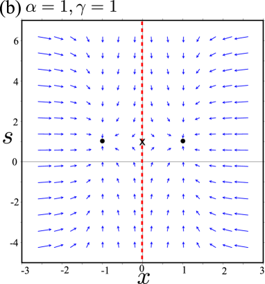
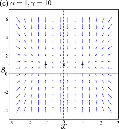
Figure 3: (Color online) Vector field plots of Eq. (21) with $\alpha=1$ and (a) $\gamma=0.1$, (b) $\gamma=1$, and (c) $\gamma=10$. There are three fixed points at $(\pm 1,\alpha)$ (stables points) and $(0,\alpha)$ (a saddle point), which are denoted by filled circles and crosses, respectively. The dotted line is a separatix, which separates the two basins.

Let $\tau_{s}$ be MFPT to the separatix ($x=0$). For sufficiently low noise intensity, MFPT $\tau_{s}$ can be well approximated by an eigenvalue Vollmer:1983:EigenvalueEscape ; Jung:1993:PeriodicSystem ; Jung:1989:ThermalActivation ; Bartussek:1995:SurmountWell :

$$\tau_{s}=\frac{1}{2r}=\frac{1}{\lambda_{1}},$$ (24)

where $r$ is the escape rate and $\lambda_{1}$ is the smallest non-vanishing eigenvalue of the FPE operator $\mathscr{L}_{0}$ [Eq. (5)]. Equation (24) gives a reliable approximation when the noise intensity is sufficiently small and $\lambda_{1}$ is well separated from the remaining eigenvalues [$\lambda_{n}$ ($n\geq 2$)]. The eigenvalue problem is represented by the equation

$$\mathscr{L}_{0}\phi(x,s)=-\lambda\phi(x,s),$$ (25)

where $\lambda$ and $\phi(x,s)$ are eigenvalues and eigenfunctions, respectively. To calculate the eigenvalues, we employ CSE as in the case of stationary distributions. According to the symmetry $x\rightarrow-x$ in $\mathscr{L}_{0}$, the eigenfunctions $\phi(x,s)$ have even [$\phi^{\mathrm{e}}(-x,s)=\phi^{\mathrm{e}}(x,s)$] or odd [$\phi^{\mathrm{o}}(-x,s)=-\phi^{\mathrm{o}}(x,s)$] parity symmetry. The even case expansion is identical to Eq. (13), and the odd case admits the following expansion:

$$\phi^{\mathrm{o}}(x,s)=\varphi_{0}(x)\psi_{0}(s)\sum_{k=0}^{K}\sum_{\ell=0}^{L}C_{k,\ell}\varphi_{2k+1}(x)\psi_{\ell}(s).$$ (26)

In the same procedure as that for stationary distributions, the even and odd cases of Eq. (25) can be reduced to linear algebraic equations. By using CSE, Eq. (25) for the odd case is calculated as

$$C_{k,\ell}\left\{2k+1-\frac{3}{2\zeta^{2}}(2k+1)^{2}-\gamma\ell\right\}-C_{k+1,\ell}\frac{2k+1}{2\zeta^{2}}\sqrt{(2k+2)(2k+3)}$$

$$+C_{k-1,\ell}\sqrt{2k(2k+1)}\left[1-\frac{3k}{\zeta^{2}}+2\zeta^{2}D_{x}\left\{\alpha^{2}+2D_{s}\left(\ell+\frac{1}{2}\right)\right\}\right]$$

$$-C_{k-2,\ell}\frac{1}{2\zeta^{2}}\sqrt{(2k+1)2k(2k-1)(2k-2)}+2C_{k-1,\ell+2}\zeta^{2}D_{x}D_{s}\sqrt{2k(2k+1)(\ell+1)(\ell+2)}$$

$$+2C_{k-1,\ell-2}\zeta^{2}D_{x}D_{s}\sqrt{2k(2k+1)\ell(\ell-1)}+4C_{k-1,\ell-1}\zeta^{2}D_{x}\alpha\sqrt{2D_{s}k(2k+1)\ell}$$

$$+4C_{k-1,\ell+1}\zeta^{2}D_{x}\alpha\sqrt{2D_{s}k(2k+1)(\ell+1)}.$$

$$=-\lambda C_{k,\ell}.$$ (27)

Equation (25) is now transformed into a linear algebraic eigenvalue problem, which can be solved with general linear algebraic eigenvalue solvers.

In practical calculation of Eq. (27), we increase $K$ and $L$ until the eigenvalues converge. In addition, we carry out MC simulations to verify the reliability of the eigenvalue-based approximation. MFPT of MC is calculated from the average of the first passage time (FPT) of $20000$ escape events. For sufficiently small noise intensity, $\tau_{s}$ can be approximated by MFPT $\tau$ from $-1$ to $0$ because the MFPT dependence on starting points exists only in a narrow boundary layer around the separatix Jung:1993:PeriodicSystem . In MC calculation, the initial value is $x=-1$, and $s$ has a Gaussian distribution $\mathcal{N}(\alpha,D_{s})$ with mean $\alpha$ and variance $D_{s}$. Fig. 4 shows the MFPT ($\tau_{s}$) dependence on $\gamma$ and $\rho$; the theoretical results obtained using CSE are denoted by lines, and the MC results are denoted by symbols.

Our model includes four parameters: $\gamma$, $\alpha$, $D_{x}$, and $D_{s}$. In our model calculations, we use $\gamma$, $\rho$, $Q$, and $D_{x}$ as the given parameters, where $Q$ and $\rho$ are defined by Eqs. (9) and (11), respectively. When these four parameters are given, $\alpha$ and $D_{s}$ are uniquely determined as $\alpha=\sqrt{Q/\{D_{x}(1+\rho)\}}$ and $D_{s}=\rho Q/\{D_{x}(1+\rho)\}$. First, we investigate the $\gamma$ dependence of MFPT with $D_{x}=1$, $Q=0.08$, and various $\rho$ values. Fig. 4(a) shows MFPT as a function of $\gamma$ with four $\rho$ values: $\rho=0.01$ (solid line and circles), $\rho=0.1$ (dotted line and squares), $\rho=1$ (dot-dashed line and triangles), and $\rho=100$ (dot-dot-dashed line and crosses). From Fig. 4(a), $\tau_{s}$ is U-shaped and has a minimum around $\gamma\simeq 1$, which can be accounted for by an RA effect. The conventional RA phenomenon occurs in a bistable potential subject to white noise, where the potential fluctuates owing to time-correlated stochastic processes. On the other hand, the RA observed in Fig. 4(a) is induced by the noise intensity fluctuation. Because MFPT increases with increasing potential wall height or decreasing noise intensity (or vice versa), the effect of noise intensity fluctuation on MFPT is similar to that of potential fluctuation. This correspondence can qualitatively explain the occurrence of the RA phenomenon in the present model. RA induced by a noise intensity fluctuation has been reported previously Iwaniszewski:2008:RAtemperature ; it was realized by the random telegraph process. As expected, the $\rho=0.01$ case shows a very small RA effect because the noise intensity fluctuation is very weak in this case. For larger $\rho$, the RA effect is larger because the noise intensity fluctuation increases with $\rho$ [Fig. 1]. In contrast, the RA effects of $\rho=1$ and $\rho=100$ are nearly similar. Remarkably, the effect of RA for $\rho=100$ is not larger than that for $\rho=1$, even though the noise intensity fluctuation is stronger for $\rho=100$ (Fig. 1(c) and (d)).

Next, we calculate the $\rho$ dependence of MFPT by varying $\rho$ while keeping the effective intensity $Q$ constant. Fig. 4(b) shows MFPT as a function of $\rho$ with four $\gamma$ values: $\gamma=0.3$ (solid line and circles), $\gamma=1$ (dotted line and squares), $\gamma=10$ (dot-dashed line and triangles), and $\gamma=100$ (dot-dot-dashed line and crosses). For $\gamma=0.3$, $\tau_{s}$ decreases as a function of $\rho$. On the other hand, $\tau_{s}$ has a minimum around $\rho\sim 1$ for $\gamma=1$, $10$, and $100$ (the depth of the minimum is smaller for larger $\gamma$). As explained, the RA phenomenon is referred to as the existence of the minimum as a function of the relaxation rate. The strength of the RA effect can be measured by the magnitude of the minima. In all $\rho$ cases in Fig. 4(a), MFPT is minimum around $\gamma\simeq 1$. Therefore, MFPT in Fig. 4(b) with $\gamma=1$ (dotted line) can be identified as the strength of the RA effect as a function of $\rho$. This indicates that the strength of the RA effect increases with $\rho$, up to $\rho\simeq 1$. A further increase in $\rho$ does not increase the strength of the RA effect.

In Fig. 4, the theoretical results obtained using CSE (lines) are in agreement with MC simulations (symbols) for all cases; this verifies the reliability of the approximation scheme.

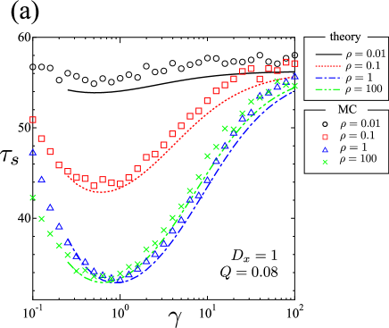
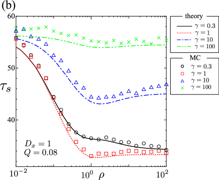
Figure 4: (Color online) MFPT $\tau_{s}$ as a function of (a) the relaxation rate $\gamma$ and (b) the squared variation coefficient $\rho$. The lines and symbols denote results of CSE and MC, respectively. (a) $D_{x}=1$ and $Q=0.08$ with $\rho=0.01$ (solid line and circles), $0.1$ (dotted line and squares), $1$ (dot-dashed line and triangles), and $100$ (dot-dot-dashed line and crosses). (b) $D_{x}=1$ and $Q=0.08$ with $\gamma=0.3$ (solid line and circles), $1$ (dotted line and squares), $10$ (dot-dashed line and triangles), and $100$ (dot-dot-dashed line and crosses). The MC results are calculated as averages of $20000$ escape events.

V Stochastic Resonance

Next, we study SR Benzi:1981:SR ; McNamara:1989:SR ; Jung:1990:MFCforPeriodic ; Jung:1991:AmpSR ; Gammaitoni:1998:SR ; Jia:2001:SRwithAddMult ; Mantegna:2000:LinNlinSR ; McDonnell:2008:SRBook ; McDonnell:2009:SR ; Agudov:2010:MonostableSR in our model. SR is an intriguing phenomenon, and it plays an important role in systems accompanied by noise; hence, it has been studied extensively in various configurations. In particular, biological applications of SR have attracted considerable attention, and they have been confirmed experimentally and theoretically Longtin:1991:SRinNeuron ; Hanggi:2002:SRinBio ; Priplata:2002:SRinBalance ; Priplata:2003:ValanceControl because biological mechanisms occur in noisy environments. We calculate the spectral amplification factor of SR with a periodic input under additive SIN. Specifically, we employ linear response approximation Dykman:1993:LRinSR to calculate the quantity. For a sufficiently small driving force, linear response approximation can be used to investigate SR.

We assume that the system of interest is modulated by an external input $\varepsilon\exp(-\mathrm{i}\Omega t)$, where $\varepsilon$ and $\Omega$ are the input strength and the angular frequency, respectively. A Langevin equation is given by

$$\frac{dx}{dt}=f(x)+\varepsilon\exp(-\mathrm{i}\Omega t)+s\xi_{x}(t),$$ (28)

and Eq. (2), where $f(x)=x-x^{3}$. The FPE of Eqs. (28) and (2) is

$$\frac{\partial}{\partial t}P(x,s;t)=\mathscr{L}_{p}P(x,s;t),$$ (29)

with

$$\mathscr{L}_{p}=\mathscr{L}_{0}+\mathscr{L}_{1}\varepsilon\exp(-\mathrm{i}\Omega t),\hskip 10.00002pt\mathscr{L}_{1}=-\frac{\partial}{\partial x},$$ (30)

where $\mathscr{L}_{0}$ is defined in Eq. (5). We assume that $\varepsilon$ is sufficiently small for the system to be well approximated by the linear response. Let $P_{as}(x,s;t)$ be an asymptotic solution ($t\rightarrow\infty$) of Eq. (29). According to the Floquet theorem, $P_{as}(x,s;t)$ is a periodic function having the same period as the input:

$$P_{as}(x,s;t)=P_{as}(x,s;t+T),$$ (31)

where $T$ is the period [$T=2\pi/\Omega$]. According to Eq. (31) and the linear response approximation, we can expand $P_{as}(x,s;t)$ as

$$P_{as}(x,s;t)=P_{0}(x,s)+P_{1}(x,s)\varepsilon\exp(-\mathrm{i}\Omega t).$$ (32)

From a normalization condition, $P_{1}(x,s)$ must satisfy

$$\int dx\int ds\,P_{1}(x,s)=0.$$ (33)

Substituting Eq. (32) into Eq. (29) and comparing the order of $\varepsilon$, we obtain the following coupled equations:

$$O(1) \mathscr{L}_{0}P_{0}(x,s)=0,$$ (34)

$$O(\varepsilon) \mathscr{L}_{0}P_{1}(x,s)+\mathscr{L}_{1}P_{0}(x,s)=-\mathrm{i}\Omega P_{1}(x,s).$$ (35)

Eq. (34) is identical to the equation for stationary distributions [Eq. (12)]. Following the procedure for stationary distributions (Sec. III), we expand $P_{1}(x,s)$ in terms of the orthonormal complete set. Using the relation $P_{as}(x,s;t)=P_{as}(-x,s;t+T/2)$ in Eq. (30), $P_{1}(x,s)$ admits the odd symmetry expansion:

$$P_{1}(x,s)=\varphi_{0}(x)\psi_{0}(s)\sum_{k=0}^{K}\sum_{\ell=0}^{L}G_{k,\ell}\varphi_{2k+1}(x)\psi_{\ell}(s),$$ (36)

where $G_{k,\ell}$ are coefficients. Note that Eq. (36) automatically satisfies Eq. (33) because of the orthonormality. Following the same procedures as those in Secs. III and IV, Eqs. (34) and (35) can be represented as the following linear algebraic equation in terms of $G_{k,\ell}$:

$$0 = \zeta\sqrt{2(2k+1)}C_{k,\ell}+G_{k,\ell}\left\{2k+1-\frac{3}{2\zeta^{2}}(2k+1)^{2}-\gamma\ell+\mathrm{i}\Omega\right\}$$ (37)

$$+G_{k-1,\ell}\sqrt{2k(2k+1)}\left[1-\frac{3k}{\zeta^{2}}+2\zeta^{2}D_{x}\left\{\alpha^{2}+2D_{s}\left(\ell+\frac{1}{2}\right)\right\}\right]$$

$$-G_{k+1,\ell}\frac{2k+1}{2\zeta^{2}}\sqrt{(2k+2)(2k+3)}-G_{k-2,\ell}\frac{1}{2\zeta^{2}}\sqrt{(2k+1)2k(2k-1)(2k-2)}$$

$$+2G_{k-1,\ell+2}\zeta^{2}D_{x}D_{s}\sqrt{2k(2k+1)(\ell+1)(\ell+2)}+2G_{k-1,\ell-2}\zeta^{2}D_{x}D_{s}\sqrt{2k(2k+1)\ell(\ell-1)}$$

$$+4G_{k-1,\ell-1}\zeta^{2}D_{x}\alpha\sqrt{2D_{s}k(2k+1)\ell}+4G_{k-1,\ell+1}\zeta^{2}D_{x}\alpha\sqrt{2D_{s}k(2k+1)(\ell+1)}.$$

$C_{k,\ell}$ has already been calculated in Eq. (18) for the stationary distributions.

From Eq. (32), the time-dependent asymptotic average of $x$ is given by

$$\left\langle x(t)\right\rangle_{as} = \int dx\int ds\,xP_{as}(x,s;t),$$ (38)

$$= \left\langle x\right\rangle_{0}+\left\langle x\right\rangle_{1}\varepsilon\exp(-\mathrm{i}\Omega t),$$

with

$$\left\langle x\right\rangle_{0}=\int dx\int ds\,xP_{0}(x,s),\hskip 10.00002pt\left\langle x\right\rangle_{1}=\int dx\int ds\,xP_{1}(x,s),$$

where $\left\langle x\right\rangle_{0}=0$ owing to the symmetry. The susceptibility $\chi$ is defined as the proportional coefficient of the input signal, which is given by $\chi=\left\langle x\right\rangle_{1}.$ There are several approaches to calculating the susceptibility, e.g., the fluctuation-dissipation relation Jung:1993:PeriodicSystem or the moment method Evstigneev:2001:MM4Periodic ; Kang:2003:DuffSRMoment . Using the orthonormal and complete relations, the susceptibility is

$$\chi=\frac{G_{0,0}}{\sqrt{2}\zeta}.$$ (39)

Let us consider a cosinusoidal input $\varepsilon\cos(\Omega t)$. $\left\langle x(t)\right\rangle_{as}$ for this case is

$$\left\langle x(t)\right\rangle_{as}=\left\langle x\right\rangle_{0}+|\chi|\varepsilon\cos(\Omega t+\theta),\hskip 10.00002pt\theta=-\arctan\left(\frac{\mathrm{Im}(\chi)}{\mathrm{Re}(\chi)}\right),$$ (40)

where $\theta$ is the phase. We evaluate the spectral amplification as $|\chi|^{2}=|G_{0,0}|^{2}/(2\zeta^{2})$.

We perform MC simulations to verify the reliability of the linear response approximation. For MC simulations, a method in Ref. Li:2009:MultiplicativeSR was employed. The averages of $2000$ trajectories were calculated and the susceptibility was estimated by their variance [Eq. (40)] (the method of moments estimation). Fig. 5 shows $\left\langle x(t)\right\rangle_{as}$ calculated by Eqs. (39) and (40) (solid line) and MC simulations (circles). We observe excellent agreement between them, which verifies the reliability of the linear response approximation.

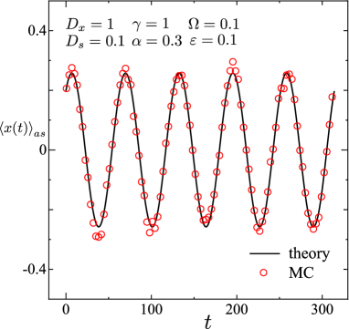
Figure 5: (Color online) $\left\langle x(t)\right\rangle_{as}$ of CSE results [Eqs. (39) and (40)] (solid line) and MC simulations as the average of $2000$ trajectories (circles). The parameters are $D_{x}=1$, $D_{s}=0.1$, $\gamma=1$, $\alpha=0.3$, and $\Omega=0.1$, and $\varepsilon=0.1$ for MC.

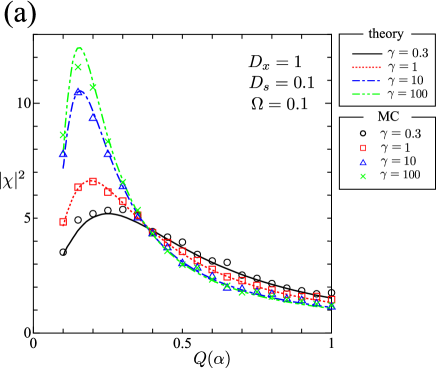
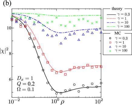
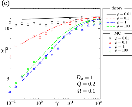
Figure 6: (Color online) (a) Spectral amplification factor $|\chi|^{2}$ as a function of (a) the effective noise intensity $Q(\alpha)$ (vary $\alpha$ while keeping $D_{s}$ constant), (b) the square variation coefficient $\rho$, and (c) the relaxation rate $\gamma$. The lines and symbols denote CSE and MC results, respectively. (a) $D_{x}=1$, $D_{s}=0.1$ and $\Omega=0.1$ with $\gamma=0.3$ (solid line and circles), $1$ (dotted line and squares), $10$ (dot-dashed line and triangles), and $100$ (dot-dot-dashed line and crosses). (b) $D_{x}=1$, $Q=0.2$ and $\Omega=0.1$ with $\gamma=0.3$ (solid line and circles), $1$ (dotted line and squares), $10$ (dot-dashed line and triangles), and $100$ (dot-dot-dashed line and crosses). (c) $D_{x}=1$, $Q=0.2$, and $\Omega=0.1$ with $\rho=0.01$ (solid line and circles), $0.1$ (dotted line and squares), $1$ (dot-dashed line and triangles), and $100$ (dot-dot-dashed line and crosses). MC results with $\varepsilon=0.1$ are calculated using the variance of the average of $2000$ trajectories (the method of moments estimation).

Fig. 6 shows the dependence of the spectral amplification factor $|\chi|^{2}$ on $Q$, $\rho$, and $\gamma$, where theoretical results obtained using CSE are denoted by lines and MC results are denoted by symbols. The MC results were in good agreement with those of CSE, verifying their reliability.

Specifically, Fig. 6(a) shows the $|\chi|^{2}$ dependence on $Q(\alpha)=D_{x}(D_{s}+\alpha^{2})$ ($\alpha$ is varied while keeping $D_{x}$ and $D_{s}$ constant) with four $\gamma$ values: $\gamma=0.3$ (solid line and circles), $\gamma=1$ (dotted line and squares), $\gamma=10$ (dot-dashed line and triangles), and $\gamma=100$ (dot-dot-dashed line and crosses) with $D_{x}=1$, $D_{s}=0.1$, and $\Omega=0.1$. Here, $|\chi|^{2}$ achieves a maximum around $Q(\alpha)=0.2$, and the maximum is larger for larger $\gamma$. SIN approaches white noise for $\gamma\rightarrow\infty$, indicating that the strength of the SR effect is maximized under white noise. On the other hand, $|\chi|^{2}$ in the range $Q(\alpha)\gtrsim 0.4$ has a different tendency, i.e., $|\chi|^{2}$ is larger for smaller $\gamma$. Although the peaks of $|\chi|^{2}$ at $Q(\alpha)\simeq 0.2$ are smaller for smaller $\gamma$, SIN can induce better performance when the noise intensity exceeds $Q(\alpha)\simeq 0.4$.

Next, we calculate $|\chi|^{2}$ as a function of $\rho$ with four $\gamma$ values: $\gamma=0.3$ (solid line and circles), $\gamma=1$ (dotted line and squares), $\gamma=10$ (dot-dashed line and triangles) and $\gamma=100$ (dot-dot-dashed line and crosses). We vary $\rho$ while keeping the effective noise intensity $Q$ constant. Because the spectral amplification factor $|\chi|^{2}$ is maximum as a function of the effective noise intensity in SR, its strength can be measured by the magnitude of the maxima. The maxima in Fig. 6(a) are located around $Q\simeq 0.2$; hence, we fixed $Q=0.2$ and investigated $|\chi|^{2}$ dependence on $\rho$ in Fig. 6(b) ($D_{x}$ and $\Omega$ are the same as as those in Fig. 6(a)). Accordingly, $|\chi|^{2}$ of Fig. 6(b) can be identified as the strength of the SR effect as a function of $\rho$. Because SIN reduces to white noise as $\gamma\rightarrow\infty$, $|\chi|^{2}$ as a function of $\rho$ does not change for $\gamma=100$. On the other hand, $|\chi|^{2}$ is more strongly affected by $\rho$ for smaller $\gamma$. SIN also reduces to white noise as $\rho\rightarrow 0$, and $|\chi|^{2}$ increases as $\rho\rightarrow 0$ in all cases. We observe non-monotonic behavior of $|\chi|^{2}$ as a function of $\rho$, i.e., the strength of the SR effect is minimized around $\rho\simeq 1$. Remarkably, the effect of the input signal is minimized around $\rho\simeq 1$, even though the strength of the noise intensity fluctuation is monotonic as a function of $\rho$.

Fig. 6(c) shows $|\chi|^{2}$ as a function of $\gamma$ for four $\rho$ values: $\rho=0.01$ (solid line and circles), $\rho=0.1$ (dotted-line and squares), $\rho=1$ (dot-dashed line and triangles), and $\rho=100$ (dot-dot-dashed line and crosses) with $D_{x}=1$, $Q=0.2$, and $\Omega=0.1$. In all cases, $|\chi|^{2}$ increases as a function of $\gamma$; therefore, the SR effect achieves a maximum under white noise.

VI Discussion

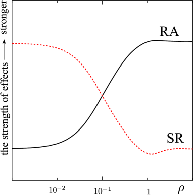
Figure 7: (Color online) Illustrative description of the strength of the RA and SR effects as a function of the squared variation coefficient $\rho$. We observe a trade-off relation between the strength of RA and SR.

In Secs. IV and V, we have shown that the strength of the RA and SR effects exhibits non-monotonic behavior as a function of the squared variation coefficient $\rho$. Furthermore, the strength of RA and SR effects is enhanced in different $\rho$ regions. The strength of the RA effect is maximum around $\rho\gtrsim 1$, whereas that of the SR effect is stronger for $\rho\lesssim 10^{-2}$. On the other hand, the strength of the SR and RA effects is very weak in regions of $\rho\simeq 1$ and $\rho\lesssim 10^{-2}$, respectively. These results shows that strength of these two effects has a trade-off relation in terms of $\rho$. An illustrative description of the trade-off relation between the strength of RA and SR effects is shown in Fig. 7, where the solid and dotted lines represent the strength of the RA and SR effects, respectively, as a function of $\rho$.

Langevin equations have been extensively applied to stochastic biochemical reactions such as gene expression Koern:2005:GeneNoiseReview and neuronal response. In a zeroth-order approximation, these biological mechanisms can be modeled using a bistable potential Wilhelm:2009:Bistability . Biological mechanisms are subject to many fluctuations having different time-scales. It has been reported theoretically and experimentally that RA and SR are expected to play important roles in biological mechanisms. RA can minimize the delays in signal detection, which improves the response to signals. On the other hand, SR is responsible for accurate signal detection in noisy environments. These two factors are important in signal transmission, and our results indicate that their importance can be tuned with $\rho$. The results presented above may provide us with a new insight into the analyses of stochastic aspects of biological mechanisms.

VII Concluding Remarks

In the present paper, we employed CSE to calculate stationary distributions, MFPT, and the spectral amplification factor. In our previous study Hasegawa:2010:SIN , we used adiabatic elimination to derive a time evolution equation. CSE is advantageous in that the ranges of the relaxation-rate $\gamma$ and the noise intensity are not limited, as opposed to the adiabatic elimination-based method, which is valid for $\gamma\gg 1$. In addition, CSE enables us to calculate quantities such as MFPT and the spectral amplification factor. On the other hand, using adiabatic elimination, we can calculate stationary distributions in the closed form, and it can be used for general non-linear drift terms. In contrast, CSE can only handle polynomial drift terms, for which stationary distributions are obtained by a numerical method. Both approaches are complementary. From the MFPT calculation, we identified the RA phenomenon as a function of $\gamma$. We also showed that the strength of the RA effect is highly dependent on the squared variation coefficient $\rho$, and that the strength of the SR effect as a function of $\rho$ is minimum around $\rho\simeq 1$. These results indicate that $\rho$, the ratio between the variance and mean of the noise intensity modulating process [Eq. (11)], has a crucial impact on the RA and SR effects.

Because CSE can be used for polynomial drift terms with arbitrary magnitudes of relaxation rate and noise intensity, the analysis described in this paper can be applied to various real-world phenomena. Furthermore, we focused on periodic SR, in which the system of interest is modulated by a periodic input. With regard to biological cases, the investigation of aperiodic SR Collins:1995:ASRinExcite ; Collins:1996:AperiodicSR is important. We plan to investigate this subject in the future.

Appendix A Correlation function

Here, we calculate the correlation function of SIN. By definition, the correlation function is given by

$$\left\langle s(t)\xi_{x}(t)s(t^{\prime})\xi_{x}(t^{\prime})\right\rangle=\int dsds^{\prime}d\xi_{x}d\xi_{x}^{\prime}\,\left[ss^{\prime}\xi_{x}\xi_{x}^{\prime}P(s,\xi_{x};t|s^{\prime},\xi_{x}^{\prime};t^{\prime})P(s^{\prime},\xi_{x}^{\prime};t^{\prime})\right].$$ (41)

Since $s(t)$ and $\xi_{x}(t)$ are independent, Eq. (41) becomes

$$\left\langle s(t)\xi_{x}(t)s(t^{\prime})\xi_{x}(t^{\prime})\right\rangle = \int dsds^{\prime}d\xi_{x}d\xi_{x}^{\prime}\,\left[ss^{\prime}\xi_{x}\xi_{x}^{\prime}P(s;t|s^{\prime};t^{\prime})P(s^{\prime};t^{\prime})P(\xi_{x};t|\xi_{x}^{\prime};t^{\prime})P(\xi_{x}^{\prime};t^{\prime})\right],$$ (42)

$$= \left\langle s(t)s(t^{\prime})\right\rangle\left\langle\xi_{x}(t)\xi_{x}(t^{\prime})\right\rangle,$$

where the correlation function of $s(t)$ is calculated as

$$\left\langle s(t)s(t^{\prime})\right\rangle=D_{s}\exp\left(-\gamma|t-t^{\prime}|\right)+\alpha^{2}.$$ (43)

From Eqs. (42) and (43), we obtain

$$\left\langle s(t)\xi_{x}(t)s(t^{\prime})\xi_{x}(t^{\prime})\right\rangle = 2D_{x}\left\{D_{s}\exp\left(-\gamma|t-t^{\prime}|\right)+\alpha^{2}\right\}\delta(t-t^{\prime}),$$ (44)

$$= 2D_{x}(D_{s}+\alpha^{2})\delta(t-t^{\prime}),$$

$$= 2Q\delta(t-t^{\prime}),$$ (45)

where $Q$ is the effective intensity defined by Eq. (9). From Eq. (45), the intensity of SIN is in agreement with the effective intensity $Q$, which is calculated via adiabatic elimination Hasegawa:2010:SIN .

References

- (1) B. Novák, J. J. Tyson, Nat. Rev. 9 (2008) 981.
- (2) J. Hull, A. White, J. Financ. 42 (1987) 281.
- (3) S. L. Heston, Rev. Financ. Stud. 6 (1993) 327.
- (4) A. A. Drăgulescu, V. M. Yakovenko, Quant. Finance 2 (2002) 443.
- (5) K. Andersson, Tech. rep., Department of Mathematics Uppsala University, U.U.D.M. Project Report 2003:18 (2003).
- (6) G. Wilk, Z. Włodarczyk, Phys. Rev. Lett. 84 (2000) 2770.
- (7) C. Beck, Phys. Rev. Lett. 87 (2001) 180601.
- (8) C. Beck, E. G. D. Cohen, Physica A 322 (2003) 267.
- (9) C. Beck, Prog. Theor. Phys. Suppl. 162 (2006) 29.
- (10) C. Beck, Braz. J. Phys. 39 (2009) 357.
- (11) C. Beck, Phil. Trans. R. Soc. A 369 (2011) 453.
- (12) P. Jizba, H. Kleinert, Phys. Rev. E 78 (2008) 031122.
- (13) S. M. D. Queirós, Braz. J. Phys. 38 (2008) 203.
- (14) Y. Hasegawa, M. Arita, Physica A 389 (2010) 4450.
- (15) R. F. Rodríguez, I. Santamaría-Holek, Physica A 385 (2007) 456.
- (16) E. V. der Straeten, C. Beck, arXiv:1012.4631 (2010).
- (17) S. M. D. Queirós, C. Tsallis, Eur. Phys. J. B 48 (2005) 139.
- (18) Y. Hasegawa, M. Arita, Physica A 390 (2011) 1051.
- (19) K. Kaneko, Prog. Theor. Phys. 66 (1976) 129.
- (20) H. Risken, The Fokker–Planck Equation: Methods of Solution and Applications, 2nd Edition, Springer, 1989.
- (21) C. R. Doering, J. C. Gadoua, Phys. Rev. Lett. 69 (1992) 2318.
- (22) U. Zürcher, C. R. Doering, Phys. Rev. E 47 (1993) 3862.
- (23) M. Marchi, F. Marchesoni, L. Gammaitoni, E. Menichella-Saetta, S. Santucci, Phys. Rev. E 54 (1996) 3479.
- (24) M. Boguñá, J. M. Porrà, J. Masoliver, K. Lindenberg, Phys. Rev. E 57 (1998) 3990.
- (25) R. N. Mantegna, B. Spagnolo, Phys. Rev. Lett. 84 (2000) 3025.
- (26) A. Fiasconaro, B. Spagnolo, Phys. Rev. E 83 (2011) 041122.
- (27) S. Denisov, P. Hänggi, J. L. Mateos, Am. J. Phys. 77 (2009) 602.
- (28) G. Bonanno, D. Valenti, B. Spagnolo, Phys. Rev. E 75 (2007) 016106.
- (29) R. N. Mantegna, B. Spagnolo, Phys. Rev. Lett. 76 (1996) 563.
- (30) B. Spagnolo, N. V. Agudov, A. A. Dubkov, Acta Phys. Pol. B 35 (2004) 1419.
- (31) A. A. Dubkov, N. V. Agudov, B. Spagnolo, Phys. Rev. E 69 (2004) 061103.
- (32) A. Fiasconaro, B. Spagnolo, Phys. Rev. E 80 (2009) 041110.
- (33) J. Iwaniszewski, A. Wozinski, Eur. Phys. Lett. 82 (2008) 50004.
- (34) P. Hänggi, P. Jung, F. Marchesoni, J. Stat. Phys. 54 (1989) 1367.
- (35) H. D. Vollmer, H. Risken, Z. Phys. B 52 (1983) 259.
- (36) P. Jung, Phys. Rep. 234 (1993) 175.
- (37) P. Jung, Z. Phys. B 76 (1989) 521.
- (38) R. Bartussek, A. J. R. Madureira, P. Hänggi, Phys. Rev. E 52 (3) (1995) R2149.
- (39) R. Benzi, A. Sutera, A. Vulpiani, J. Phys. A 14 (1981) L453.
- (40) B. McNamara, K. Wiesenfeld, Phys. Rev. A 39 (1989) 4854.
- (41) P. Jung, P. Hänggi, Phys. Rev. A 41 (1990) 2977.
- (42) P. Jung, P. Hänggi, Phys. Rev. A 44 (1991) 8032.
- (43) L. Gammaitoni, P. Hänggi, P. Jung, F. Marchesoni, Rev. Mod. Phys. 70 (1998) 223.
- (44) Y. Jia, X.-p. Zheng, X.-m. Hu, J.-r. Li, Phys. Rev. E 63 (2001) 031107.
- (45) R. N. Mantegna, B. Spagnolo, M. Trapanese, Phys. Rev. E 63 (2000) 011101.
- (46) M. D. McDonnell, N. G. Stocks, C. E. M. Pearce, D. Abbott, Stochastic resonance, Cambridge University Press, 2008.
- (47) M. D. McDonnell, D. Abbott, PLoS Comput. Biol. 5 (2009) e1000348.
- (48) N. V. Agudov, A. V. Krichigin, D. Valenti, B. Spagnolo, Phys. Rev. E 81 (2010) 051123.
- (49) A. Longtin, A. Bulsara, F. Moss, Phys. Rev. Lett. 67 (1991) 656.
- (50) P. Hanggi, ChemPhysChem 3 (2002) 285.
- (51) A. Priplata, J. Niemi, M. Salen, J. Harry, L. A. Lipsitz, J. J. Collins, Phys. Rev. Lett. 89 (2002) 238101.
- (52) A. A. Priplata, J. B. Niemi, J. D. Harry, L. A. Lipsitz, J. J. Collins, Lancet 362 (2003) 1123.
- (53) M. I. Dykman, H. Haken, G. Hu, D. G. Luchinsky, R. Mannella, P. V. E. McClintock, C. Z. Ning, N. D. Stein, N. G. Stocks, Phys. Lett. 180 (1993) 332.
- (54) M. Evstigneev, V. Pankov, R. H. Prince, J. Phys. A 34 (2001) 2595.
- (55) Y.-M. Kang, J.-X. Xu, Y. Xie, Phys. Rev. E 68 (2003) 036123.
- (56) J.-H. Li, Commun. Theor. Phys. 51 (2009) 675.
- (57) M. Kœrn, T. C. Elston, W. J. Blake, J. J. Collins, Nat. Rev. 6 (2005) 451.
- (58) T. Wilhelm, BMC Syst. Biol. 3 (2009) 90.
- (59) J. J. Collins, C. C. Chow, T. T. Imhoff, Phys. Rev. E 52 (1995) R3321.
- (60) J. J. Collins, C. C. Chow, A. C. Capela, T. T. Imhoff, Phys. Rev. E 54 (1996) 5575.