Warm dark matter at small scales:
peculiar velocities and phase space density.

Abstract

We study the scale and redshift dependence of the power spectra for density perturbations and peculiar velocities, and the evolution of a coarse grained phase space density for (WDM) particles that decoupled during the radiation dominated stage. The (WDM) corrections are obtained in a perturbative expansion valid in the range of redshifts at which N-body simulations set up initial conditions, and for a wide range of scales. The redshift dependence is determined by the kurtosis $\beta_{2}$ of the distribution function at decoupling. At large redshift there is an enhancement of peculiar velocities for $\beta_{2}>1$ that contributes to free streaming and leads to further suppression of the matter power spectrum and an enhancement of the peculiar velocity autocorrelation function at scales smaller than the free streaming scale. Statistical fluctuations of peculiar velocities are also suppressed on these scales by the same effect. In the linearized approximation, the coarse grained phase space density features redshift dependent (WDM) corrections from gravitational perturbations determined by the power spectrum of density perturbations and $\beta_{2}$. For $\beta_{2}>25/21$ it grows logarithmically with the scale factor as a consequence of the suppression of statistical fluctuations. Two specific models for WDM are studied in detail. The (WDM) corrections relax the bounds on the mass of the (WDM) particle candidate.

I Introduction

The current paradigm of structure formation, the $\Lambda CDM$ standard cosmological model, describes large scale structure remarkably well. However, observational evidence has been accumulating suggesting that the cold dark matter (CDM) scenario of galaxy formation may have problems at small, galactic, scales.

Large scale simulations seemingly yield an over-prediction of satellite galaxiesmoore2 by almost an order of magnitudekauff ; moore ; moore2 ; klyp ; will . Simulations within the $\Lambda$CDM paradigm also yield a density profile in virialized (DM) halos that increases monotonically towards the centerfrenk ; dubi ; moore2 ; bullock ; cusps and features a cusp, such as the Navarro-Frenk-White (NFW) profilefrenk or more general central density profiles $\rho(r)\sim r^{-\beta}$ with $1\leq\beta\lesssim 1.5$moore ; frenk ; cusps . These density profiles accurately describe clusters of galaxies but there is an accumulating body of observational evidencedalcanton1 ; van ; swat ; gilmore ; salucci ; battaglia ; deblok ; kravstov suggesting that the central regions of dark matter (DM)-dominated dwarf spheroidal satellite (dSphs) galaxies feature smooth cores instead of cusps as predicted by (CDM). Some observations suggestsalucci2 that the mass distribution of spiral disk galaxies can be best fit by a cored Burkert-type profilesalucci2 . This difference is known as the core-vs-cusp problemdeblok ; kravstov . The case for core-dominated halos has been recently bolstered by the analysis of rotation curves from the THINGS surveythings .

Warm dark matter (WDM) particles were invokedmooreWDM ; turokWDM ; avila as possible solutions to the discrepancies both in the over abundance of satellite galaxies and as a mechanism to smooth out the cusped density profiles predicted by (CDM) simulations into the cored profiles that fit the observations in (dShps). (WDM) particles feature a range of velocity dispersion in between the (CDM) and hot dark matter leading to free streaming scales that smooth out small scale features and could be consistent with core radii of the (dSphs). If the free streaming scale of these particles is smaller than the scale of galaxy clusters, their large scale structure properties are indistinguishable from (CDM) but may affect the small scale power spectrumbond providing an explanation of the smoother inner profiles of (dSphs) and fewer satellites.

Furthermore recent numerical results hint to more evidence of possible small scale discrepancies with the $\Lambda CDM$ scenario: another over-abundance problem, the “emptiness of voids” tikhoklypin and the spectrum of “mini-voids”tikho , both of which may be explained by a WDM candidate. Constraints from the luminosity function of Milky Way satellitesmaccio suggest a lower limit for the mass of a WDM particle of a few $\mathrm{keV}$, a result consistent with Lyman-$\alpha$lyman ; lyman2 ; vieldwdm , galaxy power spectrumabakousha and lensing observationsmaccio2 . More recently, results from the Millenium-II simulationsawala suggest that the $\Lambda CDM$ scenario overpredicts the abundance of massive $\gtrsim 10^{10}\,M_{\odot}$ haloes, which is corrected with a WDM candidate of $m\sim 1\,\mathrm{keV}$. A model independent analysis suggests that dark matter particles with a mass in the $\mathrm{keV}$ range is a suitable (WDM) candidatehectornorma ; hecsal . Recent counterargumentskapli ; dalal seem to suggest that (WDM) cannot explain cores in (LSB) galaxies, thus the controversy continues.

In absence of conclusive evidence in favor of or against cusps or cores, and in view of the ongoing controversy and the body of emerging evidence in favor of (WDM), a deeper understanding of the small scale clustering properties of (WDM) candidates is warranted.

Motivation and goals:

Redshift dependence of the power spectrum and peculiar velocities: recent N-body simulations of WDMtikho ; maccio set up initial conditions at $z=40$maccio or $z=50$tikho with a rescaled version of the CDM power spectrum from a fit provided in ref.vieldwdm that inputs a cutoff from free streaming, however, these simulations neglected the velocity dispersion of the WDM particles in the initial conditions. We seek to understand both the redshift dependence of the matter and peculiar velocity power spectrum in this range of redshifts for a wide range of scales.

Phase space density: in a seminal article Tremaine and GunnTG provided bounds on the mass of the DM particle from phase space density considerations: whereas in absence of self-gravity the fine-grained phase space density (or distribution function) is conserved after the DM species decouples from the plasma, phase mixing theoremstheo assert that a coarse grained phase space density always diminishes as a result of phase mixing (violent relaxation)theo ; dehnen . Therefore the microscopic phase space density provides an upper bound from which constraints on the mass can be extracted. These arguments were generalized in refs.dalcanton1 ; hogan ; coldmatter ; darkmatter ; boysnudm ; hectornorma to a coarse grained phase space density obtained from moments of the microscopic distribution function. In ref.coldmatter ; darkmatter ; boysnudm ; hectornorma this coarse grained phase space density was combined with photometric observations of (dShps) to constrain the mass and the number of relativistic degrees of freedom at decoupling.

Although the microscopic phase space density, namely the distribution function, obeys the collisionless Boltzmann equation, the evolution of the coarse grained phase space density is not directly obtained from this equation (see discussion in ref.dehnen ). Although the proxy phase space density introduced in refs.dalcanton1 ; hogan ; coldmatter ; darkmatter is conserved after decoupling, its evolution does not include self-gravity. Therefore there remains the unexplored question of precisely what happens to the microscopic phase space density or its proxy introduced in refs.dalcanton1 ; hogan ; coldmatter ; darkmatter when gravitational perturbations are included in the Boltzmann equation. One aspect is clear: the perturbations of the distribution function (microscopic phase space density) feature two moments that grow under gravitational perturbations: the first moment (density perturbations) and the second moment (velocity perturbations) which are actually related via the continuity equation on sub-horizon scales. In this article we study the evolution of the coarse-grained phase space density introduced in refs.dalcanton1 ; hogan ; coldmatter ; darkmatter as a function of redshift and scale for (WDM) particles in order to assess how the original arguments are modified by gravitational perturbations, again in the regime of redshifts at which N-body simulations set up initial conditions.

Results:

Armed with the results recently obtained in ref.smallscale we obtain a perturbative expansion of the redshift corrections to the matter, peculiar velocity power spectra and evolution of a coarse-grained phase space density. This expansion is valid in the regime $z\ll z_{eq}$ for a wide range of scales and is a distinct feature of (WDM) particles. These corrections depend on the kurtosis $\beta_{2}$ of the unperturbed distribution function. Peculiar velocities contribute to the velocity dispersion and free streaming and lead to a suppression of the matter power spectrum for $\beta_{2}>1$ at scales smaller than the free streaming scale at redshifts $z\simeq 30-50$. The peculiar velocity power spectrum is enhanced at these scales and reshift leading to an increase of the peculiar velocity autocorrelation function and a suppression of statistical fluctuations. For (WDM) perturbations in the linearized approximation, it is found that the coarse grained phase space density introduced in refs.dalcanton1 ; hogan ; coldmatter ; darkmatter grows logarithmically with the scale factor for $\beta_{2}>25/21$. Two specific models of (WDM) particles motivated by particle physics are studied in detail. Implications on the bounds for the mass of the (WDM) particle are discussed.

II Preliminaries

We begin by establishing some notation and conventions that are used in the analysis. Since we focus on the region of redshift $z\gg 1$ we can safely neglect the dark energy component and we consider a radiation and matter dominated cosmology with

$$H^{2}=\frac{\dot{a}^{2}}{a^{4}}=H^{2}_{0}\left[\frac{\Omega_{r}}{a^{4}}+\frac{\Omega_{m}}{a^{3}}\right]=\frac{H^{2}_{0}\Omega_{m}}{a^{4}}\left[a+a_{eq}\right]$$ (II.1)

where the dot stands for derivative with respect to conformal time ($\eta$), the scale factor is normalized to $a_{0}=1$ today, and

$$a_{eq}=\frac{\Omega_{r}}{\Omega_{m}}\simeq\frac{1}{3229}\,.$$ (II.2)

Introducing

$$\tilde{a}=\frac{a}{a_{eq}}\,,$$ (II.3)

it follows that

$$\frac{d\,\tilde{a}}{d\eta}=\left[\frac{H^{2}_{0}\Omega_{m}}{a_{eq}}\right]^{\frac{1}{2}}\,\left[1+\tilde{a}\right]^{\frac{1}{2}}\,.$$ (II.4)

At matter-radiation equality we define

$$k_{eq}\equiv H_{eq}\,a_{eq}=\sqrt{2}\left[\frac{H^{2}_{0}\Omega_{m}}{a_{eq}}\right]^{\frac{1}{2}}=\frac{9.8\times 10^{-3}}{\mathrm{Mpc}}$$ (II.5)

corresponding to the comoving wavevector that enters the Hubble radius at matter-radiation equality, where we have used $\Omega_{m}h^{2}=0.134$WMAP7 .

We study the evolution of perturbations in the conformal Newtonian gauge

$$g_{00} = -a^{2}(\eta)\Big{[}1+2\psi(\vec{x},\eta)\Big{]}$$ (II.6)

$$g_{ij} = a^{2}(\eta)\Big{[}1-2\phi(\vec{x},\eta)\Big{]}~{}\delta_{ij}\,.$$ (II.7)

The perturbed distribution function is given by

$$f(p,\vec{x},\eta)=f_{0}(p)+F_{1}(p,\vec{x},\eta)$$ (II.8)

where $f_{0}(p)$ is the unperturbed distribution function, which after decoupling obeys the collisionless Boltzmann equation in absence of perturbations and $\vec{p},\vec{x}$ are comoving momentum and coordinates respectively. As discussed in ref.coldmatter ; darkmatter ; boysnudm the unperturbed distribution function is of the form

$$f_{0}(p)\equiv f_{0}(y;\chi_{1},\chi_{2},\cdots)$$ (II.9)

where

$$y=\frac{p}{T_{0,d}}$$ (II.10)

where $p$ is the comoving momentum and $T_{0,d}$ is the decoupling temperature today,

$$T_{0,d}=\Big{(}\frac{2}{g_{d}}\Big{)}^{\frac{1}{3}}~{}T_{CMB}\,,$$ (II.11)

with $g_{d}$ being the effective number of relativistic degrees of freedom at decoupling, $T_{CMB}=2.35\times 10^{-4}~{}\mathrm{eV}$ is the temperature of the (CMB) today, and $\chi_{i}$ are dimensionless couplings or ratios of mass scales.

We neglect stress anisotropies, in which case $\phi=\psi$ and introduce

$$\widetilde{F}(\vec{p},\vec{k},\eta)=\frac{F_{1}(\vec{p},\vec{k},\eta)}{n_{0}}~{}~{};~{}~{}\widetilde{f}(p)=\frac{f_{0}(p)}{n_{0}}$$ (II.12)

where

$$n_{0}=\int\frac{d^{3}p}{(2\pi)^{3}}\,f_{0}(p)\,,$$ (II.13)

is the background density of (DM) today. Therefore

$${\delta}(\vec{k},\eta)=\int\frac{d^{3}p}{(2\pi)^{3}}\,\widetilde{F}(\vec{k},\eta)\,.$$ (II.14)

becomes $\delta\rho_{m}/\rho_{m}$ after the DM particle becomes non-relativistic.

Introducing spatial Fourier transforms in terms of comoving momenta $\vec{k}$ (we keep the same notation for the spatial Fourier transform of perturbations), and neglecting stress anisotropies the linearized Boltzmann equation for perturbations is given byma ; dodelson ; giova ; lythbook ; weinbergbook ; ruthbook ; kodama

$$\dot{\widetilde{F}}(\vec{k},\vec{p}\,;\eta)+i\frac{k\,\mu\,p}{\epsilon(p,\eta)}~{}\widetilde{F}(\vec{k},\vec{p}\,;\eta)+\Big{(}\frac{d~{}\widetilde{f}(p)}{dp}\Big{)}\Big{[}p~{}\dot{\phi}(\vec{k},\eta)-ik\,\mu\,\epsilon(p,\eta)~{}\phi(\vec{k},\eta)\Big{]}=0$$ (II.15)

where dots stand for derivatives with respect to conformal time, $\mu=\widehat{\mathbf{k}}\cdot\widehat{\mathbf{p}}$, and $\epsilon(p,\eta)=\sqrt{p^{2}+m^{2}\,a^{2}(\eta)}$ is the conformal energy of the particle of mass $m$. The gravitational potential is determined by Einstein’s equationma ; dodelson .

As discussed in ref.smallscale for a (WDM) particle with a mass in the $\sim\,\mathrm{keV}$ range, there are three stages of evolution: I) radiation domination and the DM particle is relativistic, II) radiation domination and the DM particle is non-relativistic and III) the matter dominated stage, during which cold and warm DM particles are non-relativistic.

During stages (I) and (II) the gravitational potential is completely determined by the radiation component and the Boltzmann equation for the distribution function of the WDM particle is solved by integrating eqn. (II.15) with $\phi$ being determined by the radiation component. During stage (III) the gravitational potential is determined by the matter component and the Boltzmann equation becomes a self-consistent Vlasov-type equation.

Since the Boltzmann equation is first order in time, the solution during stages (I) and (II) becomes the initial condition for the evolution during stage (III).

In this article we focus on the evolution of peculiar velocities and phase space density during the matter dominated stage $10\leq z\lesssim z_{eq}$, corresponding to stage (III) during which dark energy can be neglected. Typical N-body simulations setup initial conditions which input the matter power spectrum from linear perturbation theory at $z\simeq 30-50$.

In this stage the WDM is non-relativistic, hence $p/\epsilon(p,\eta)=p/m\,a(\eta)$, and the Bolzmann equation simplifies by introducing the variable

$$s(\eta)=\int^{\eta}\frac{d\eta^{\prime}}{a(\eta^{\prime})}\equiv\frac{2\sqrt{2}\,u(\eta)}{k_{eq}a_{eq}}$$ (II.16)

where the dimensionless variable

$$u(\eta)=\frac{1}{2}\,\ln\Bigg{[}\frac{\sqrt{1+\tilde{a}(\eta)}-1}{\sqrt{1+\tilde{a}(\eta)}+1}\Bigg{]}~{}~{};~{}~{}u_{NR}\leq u(\eta)\leq 0\,,$$ (II.17)

is normalized so that $u(\infty)=0$ and introducedsmallscale

$$u_{NR}=\ln\Big{[}\frac{\sqrt{\tilde{a}_{NR}}}{2}\Big{]}~{}~{};~{}~{}\tilde{a}_{NR}=\langle{V}^{2}(t_{eq})\rangle^{\frac{1}{2}}\,$$ (II.18)

where $\tilde{a}_{NR}$ corresponds to the time when the particle becomes non-relativistic, and $\langle{V}^{2}(t_{eq})\rangle$ is the velocity dispersion of the DM particle at matter-radiation equality given bysmallscale

$$\langle{V}^{2}(t_{eq})\rangle^{\frac{1}{2}}\simeq 7.59\,\times 10^{-4}\,\sqrt{\overline{y^{2}}}\,\Big{(}\frac{\mathrm{keV}}{m}\Big{)}\,\Big{(}\frac{2}{g_{d}}\Big{)}^{\frac{1}{3}}\,.$$ (II.19)

In this expression $g_{d}$ is the number of relativistic degrees of freedom at decoupling and we introduced the moments

$$\overline{y^{n}}=\frac{\int_{0}^{\infty}y^{2+n}\,f_{0}(y)\,dy}{\int_{0}^{\infty}y^{2}\,f_{0}(y)\,dy}\,.$$ (II.20)

The function $u[z]$ as function of redshift is displayed in fig. (1) and

$$\tilde{a}(u)=\frac{1}{\sinh^{2}[u]}\,.$$ (II.21)

Figure 1: $u[z]$ for $z\leq z_{eq}$.

The solution of the Boltzmann equation during stage (III) is given in ref.(smallscale )

$$\widetilde{F}(\vec{k},\vec{p};s) = -\phi(\vec{k},s)\,\Big{(}p\,\frac{d\widetilde{f}(p)}{dp}\Big{)}+i\,m\,\int_{s_{NR}}^{s}ds^{\prime}\,a^{2}(s^{\prime})\,\phi(\vec{k},s^{\prime})\Big{(}\vec{k}\cdot\vec{\nabla}_{p}\widetilde{f}(p)\Big{)}\,e^{-i\frac{\vec{k}\cdot\vec{p}}{m}(s-s^{\prime})}$$ (II.22)

$$+ e^{-i\frac{\vec{k}\cdot\vec{p}}{m}(s-s_{NR})}\,\Big{[}\widetilde{F}(\vec{k},\vec{p};\eta_{NR})+\phi(\vec{k},\eta_{NR})\,\Big{(}p\,\frac{d\widetilde{f}}{dp}\Big{)}\Big{]}\,.$$

The term $\widetilde{F}(\vec{k},\vec{p};\eta_{NR})$ in the bracket in eqn. (II.22) is the solution of the Boltzmann equation at the beginning of stage (III) (end of stage (II)) its form is given in detail in ref.smallscale but is not necessary in the discussion that follows.

After radiation-matter equality when the WDM particle is non-relativistic and (DM) perturbations dominate the gravitational potential and for $k\gg k_{eq}$, the gravitational potential $\phi$ is determined by Poisson’s equationdodelson

$$\phi(k,\eta)=-\frac{3}{4}\frac{k^{2}_{eq}}{k^{2}\,\tilde{a}}\,{\delta}(\vec{k},s)$$ (II.23)

For $s>s_{eq}$, the integral in $s^{\prime}$ in (II.22) is split from $s_{NR}$ up to $s_{eq}$ and from $s_{eq}$ up to $s$. In the first integral the gravitational potential is determined by perturbations in the radiation fluid and in the second integral the gravitational potential is replaced by Poisson’s equation (II.23), leading to the result (valid for $s>s_{eq}$)smallscale

$$\widetilde{F}(\vec{k},\vec{p};s) = \frac{3}{4}\frac{k^{2}_{eq}}{k^{2}\,\tilde{a}}\,{\delta}(\vec{k},s)\,\Big{(}p\,\frac{d\widetilde{f}(p)}{dp}\Big{)}-i\,\frac{3mk^{2}_{eq}a^{2}_{eq}}{4k}\,\int_{s_{eq}}^{s}ds^{\prime}\,\tilde{a}(s^{\prime})\,{\delta}(k,s^{\prime})\,\mu\,\Big{(}\frac{d\widetilde{f}(p)}{dp}\Big{)}\,e^{-i\mu Q}$$ (II.24)

$$+ \mathcal{F}[\vec{k},\vec{p};s]\,.$$

where

$$Q=\frac{kp}{m}(s-s^{\prime})~{};~{}\mu=\widehat{\mathbf{k}}\cdot\widehat{\mathbf{p}}\,,$$ (II.25)

and $\mathcal{F}[\vec{k},\vec{p};s]$ is given by the second line in (II.22) plus the contribution from the integral between $s_{NR}$ and $s_{eq}$ (for details see ref.smallscale ).

We are interested in the corrections to the power spectra in the regime of redshift $1<z\ll z_{eq}$ corresponding to $\tilde{a}\gg 1$.

In the asymptotic limit $\tilde{a}\gg 1$ when density perturbations grow as in an Einstein-DeSitter cosmology, ${\delta}\propto\tilde{a}$, therefore in this limit and for $k\gg k_{eq}$ we can neglect the first term in (II.24). Since in this limit ${\delta}(k,s^{\prime})\propto\tilde{a}(s^{\prime})\propto(1/s^{\prime})^{2}$ the integral in eqn. (II.24) is $\propto 1/s^{3}$ and dominates all other terms in eqn. (II.24) since the last term remains finite in the limit $s\rightarrow 0$smallscale .

Therefore in the asymptotic limit $\tilde{a}\gg 1$ and for small scales $k\gg k_{eq}$ the leading contribution to the perturbation in the distribution function is given by

$$\widetilde{F}(\vec{k},\vec{p};s)\simeq-i\,\frac{3mk^{2}_{eq}a^{2}_{eq}}{4k}\,\int_{s_{eq}}^{s}ds^{\prime}\,\tilde{a}(s^{\prime})\,{\delta}(\vec{k},s^{\prime})\,\mu\,\Big{(}\frac{d\widetilde{f}(p)}{dp}\Big{)}\,e^{-i\mu Q}$$ (II.26)

With this form for the distribution function we can obtain any expectation value once ${\delta}(k,s)$ is determined from the solution of the Boltzmann equation.

In ref.smallscale it is shown that in terms of the variable $u$ defined by eqns. (II.16,II.17) $\delta$ obeys the fluid-like integro-differential equation

$$\frac{d^{2}}{du^{2}}{\delta}(k,u)-6\,\tilde{a}(u){\delta}(k,u)+\kappa^{2}{\delta}(k,u)-6\,\alpha\int_{u_{NR}}^{u}\tilde{a}(u^{\prime})\,\widetilde{\Pi}\big{[}\alpha(u-u^{\prime})\big{]}{\delta}(k,u^{\prime})\,du^{\prime}$$ (II.27)

$$= J[k,u]$$

where the inhomogeneity $J[k,u]$ is given explicitly in ref.smallscale , and

$$\widetilde{\Pi}\big{[}\alpha(u-u^{\prime})\big{]}=\frac{1}{N}\int_{0}^{\infty}yf_{0}(y)(\overline{y^{2}}-y^{2})\sin\big{[}y\,\alpha\,(u-u^{\prime})\big{]}dy~{}~{};~{}~{}N=\int_{0}^{\infty}y^{2}f_{0}(y)\,dy\,.$$ (II.28)

In the above expressions we introduced

$$\alpha=2\sqrt{2}~{}\frac{k\,T_{0,d}}{m\,k_{eq}a_{eq}}\simeq 2.15\times 10^{-3}\,\Big{(}\frac{k}{k_{eq}}\Big{)}\,\Big{(}\frac{2}{g_{d}}\Big{)}^{\frac{1}{3}}\,\Big{(}\frac{\mathrm{keV}}{m}\Big{)}\simeq 0.22\,k\,\Big{(}\frac{2}{g_{d}}\Big{)}^{\frac{1}{3}}\,\Big{(}\frac{\mathrm{keV}}{m}\Big{)}\times\big{(}\mathrm{Mpc}\big{)}\,,$$ (II.29)

and

$$\kappa\equiv\sqrt{\overline{y^{2}}}~{}\alpha\,.$$ (II.30)

In terms of the free streaming wavevectorsmallscale

$$k_{fs}=\frac{\sqrt{3}}{2}\,\frac{k_{eq}}{\langle\vec{V}^{2}(t_{eq})\rangle^{\frac{1}{2}}}=\frac{11.17}{\sqrt{\overline{y^{2}}}}\,\Big{(}\frac{m}{\mathrm{keV}}\Big{)}\,\Big{(}\frac{g_{d}}{\mathrm{2}}\Big{)}^{\frac{1}{3}}\,(\mathrm{Mpc})^{-1}\,,$$ (II.31)

it follows that

$$\kappa=\frac{\sqrt{6}k}{k_{fs}}=\frac{\sqrt{6}\,\lambda_{fs}}{\lambda}$$ (II.32)

where $\lambda_{fs}$ is the free streaming length and $\lambda$ the wavelength of the perturbation. The (CDM) limit corresponds to $\lambda_{fs}\rightarrow 0$, namely $\kappa\rightarrow 0$, therefore all the WDM corrections are in terms of $\kappa$.

In the (CDM) limit eqn.(II.27) reduces to Meszaro’s equationmesaros ; groth ; peeblesbook for (CDM) perturbations in a radiation and matter dominated cosmologysmallscale .

The power spectrum of density perturbations is given by

$$P_{\delta}(k)=Ak^{n_{s}}T^{2}(k)$$ (II.33)

where where $n_{s}=0.963$WMAP7 is the index of primordial scalar perturbations, $A$ is the amplitude and $T(k)$ is the transfer function. It is convenient to normalize the WDM power spectrum and transfer function to CDM, namely

$$P_{wdm}(k)=P_{cdm}(k)\,\overline{T}^{\,2}(k)~{}~{};~{}~{}\overline{T}(k)=\frac{T_{wdm}(k;\kappa)}{T_{cdm}(k)}$$ (II.34)

where

$$P_{cdm}(k)=Ak^{n_{s}}T^{2}_{cdm}(k)$$ (II.35)

is the (CDM) power spectrum and the dependence on WDM is encoded in the $\kappa$ dependence of $T_{wdm}(k;\kappa)$ so that $T_{wdm}(k;\kappa=0)=T_{cdm}(k)$. The dependence on $\kappa$ describes the velocity dispersion and non-vanishing free streaming length of the WDM particle.

In ref.smallscale it is shown that eqn. (II.27) can be solved in a systematic Fredholm expansion, from which the transfer function of density perturbations at $z=0$ is extracted. The leading order term is a Born-type approximation which provides a remarkably accurate approximation to the transfer function and reproduces numerical results available in the literature in several cases (for discussion and comparison seesmallscale ). The definition of the power spectrum and transfer function above are at $z=0$. We seek to study the redshift dependence for $z\lesssim 30-40$ at which N-body simulations set up initial conditions.

Asymptotically during the matter dominated era as $\tilde{a}\rightarrow\infty$ ($u\rightarrow 0$) it is foundsmallscale that $\delta(k,u)\rightarrow\tilde{a}(u)\,\delta(k,0)+\cdots$ where the dots stand for subleading terms. The leading and subleading asymptotic behavior in the $u\rightarrow 0$ ($\tilde{a}\rightarrow\infty$) limit can be obtained from eqn. (II.27). In this limit the inhomogeneity $J[k,0]$ is a finite constant (see expressions in ref.smallscale ), the integral term receives the largest contribution for $u^{\prime}\sim u\sim 0$ and in this region we find

$$-6\alpha\widetilde{\Pi}\big{[}\alpha(u-u^{\prime})\big{]}\simeq\kappa^{4}(u-u^{\prime})^{3}\Big{(}1-\beta_{2}\Big{)}+\cdots\,.$$ (II.36)

where

$$\beta_{2}=\frac{\overline{y^{4}}}{\big{(}\overline{y^{2}}\big{)}^{2}}$$ (II.37)

is the kurtosis of the distribution function of the decoupled particle, with the moments defined by eqn. (II.20), and the dots stand for terms that yield subleading corrections (see below).

Since

$$\tilde{a}(u)=\frac{1}{\sinh^{2}[u]}\sim\frac{1}{u^{2}}-\frac{1}{3}+\mathcal{O}(u^{2})\,,$$ (II.38)

we propose the asymptotic expansion

$$\delta(k,u)=\frac{\delta(k,0)}{u^{2}}+\delta_{1}(k)+\delta_{2}(k)~{}u^{2}\,\ln[-u]+\cdots\,$$ (II.39)

Introducing this expansion in eqn. (II.27) we find

$$\delta_{1}(k)=\frac{\delta(k,0)}{6}\big{[}\kappa^{2}+2\big{]}~{}~{};~{}~{}\delta_{2}(k)=-\delta(k,0)\,\frac{\kappa^{4}}{4}\Big{(}1-\beta_{2}\Big{)}\,,$$ (II.40)

where $\delta(\vec{k},0)$ is obtained from the asymptotic solution of the full eqn. (II.27). Therefore

$$\delta(\vec{k},u)=\delta(\vec{k},0)\,D[k,u]$$ (II.41)

where the wavevector dependent growth factor is found to be

$$D[k,u]=D_{cdm}[u]~{}\overline{D}[k,u]$$ (II.42)

with $D_{cdm}[u]$ being the CDM growth factor (for $\kappa=0$)

$$D_{cdm}=\frac{1}{u^{2}}\,\Bigg{[}1+\frac{u^{2}}{3}+\cdots\Bigg{]}$$ (II.43)

and

$$\overline{D}[k,u]=\Bigg{[}1+\frac{(\kappa\,u)^{2}}{6}+\frac{(\kappa\,u)^{4}}{4}(-\ln[-u])\,\Big{(}1-\beta_{2}\Big{)}+\cdots\Bigg{]}\,.$$ (II.44)

contains the WDM corrections as is manifest in the $\kappa$ dependence.

For $u\rightarrow 0$ we find

$$D_{cdm}[u]=\frac{1}{u^{2}}+\frac{1}{3}\simeq\tilde{a}+\frac{2}{3}$$

which is recognized as the growing solution of Meszaros equation for CDMmesaros ; groth ; peeblesbook . Furthermore from (II.16) we recognize that

$$-\kappa\,u=k\,l_{fs}\big{[}\frac{\sqrt{\langle p^{2}\rangle}}{m},\eta_{0},\eta\big{]}$$ (II.45)

where $l_{fs}\big{[}\frac{\sqrt{\langle p^{2}\rangle}}{m},\eta_{0},\eta\big{]}$ is the comoving free streaming distance that a particle with (comoving) velocity $\sqrt{\langle p^{2}\rangle}/m$ travels between conformal time $\eta$ and today $\eta_{0}\gg 1$. We see that up to logarithms, the expansion in powers of $\kappa\,u$ is valid at late times for wavelengths much larger than the free streaming distance that the particle would travel between that time and today.

The identification (II.45) leads to a simple physical interpretation of the first term in $\overline{D}[k,u]$: free streaming of collisionless particles suppresses the gravitational collapse of density perturbations, the longer the time scale, the farther the free streaming particles can travel away from the collapsing region erasing the perturbations. Therefore the first term reflects that at earlier times (larger values of $u$) density perturbations are larger. The second term, however, has a more interesting interpretation. As it will be discussed below, it represents the peculiar velocity contribution to free streaming induced by gravitational self-interaction (see discussion on peculiar velocity below). When $\beta_{2}>1$ the peculiar velocity contribution increases the free streaming velocity leading to a suppression of power, which counterbalances the enhancement by the first term. Which term dominates depends on the scale $k$, the free streaming wavevector, a characteristic of the WDM particle, and the redshift. This will be analyzed in two specific models below.

We emphasize that the expansion in (II.39) is valid at long time, in particular for $\kappa\,u<1$. At higher orders in the expansion, the terms that feature the $\ln(-u)$ only appear linearly in the logarithm but multiplied by higher powers of $\kappa\,u$, therefore for $|\kappa\,u|<1$ the third term in $\overline{D}$ is the leading logarithmic contribution, with higher contributions being of the form $(\kappa\,u)^{n}\,\ln(-u)~{};~{}n=6,8\cdots$. This is an important observation: in particular within the regime of validity of the perturbative expansion $|\kappa u|<1$ it is still possible that $|\kappa u\,\ln(-u)|\sim 1$ and the second term in (II.44) can balance the first term within the region of validity of the approximation.

An estimate of the range of validity is obtained from

$$0.098\leq-u[z]\leq 0.125~{}~{}for~{}~{}30\leq z\leq 50\,,$$ (II.46)

for example in the region of redshifts where initial conditions for N-body simulations are set up, the WDM corrections to the growth factor are of $\mathcal{O}(10-15\%)$ for $k\gtrsim(1-2)\,k_{fs}$ which for a species with $m\sim\mathrm{keV}$ decoupled with $g_{d}\sim 30-100$ with $\overline{y^{2}}\sim 10$ corresponds to $k\gtrsim 10-30\,(\mathrm{Mpc})^{-1}$.

There is a caveat in this analysis of the reliability of the expansion, since it applies only in the linear regime where the linearized Boltzmann equation describes the transfer function. It is conceivable that non-linear effects restrict further the regime of validity, but of course this cannot be assessed in the linear theory which is the focus of this discussion.

Using Poisson’s equation (II.23), the asymptotic behavior ${\delta}(\vec{k},u)\rightarrow{\delta}(\vec{k},0)\,\tilde{a}(u)$ and the definition of the transfer functiondodelson $T(k)$

$$\phi(k,\tilde{a}\gg 1)=\frac{9}{10}\phi_{i}(k)T(k)$$ (II.47)

where $\phi_{i}(k)$ is the primordial value of gravitational perturbations seeded by inflation. It then follows that

$${\delta}(\vec{k},0)=-\phi_{i}(\vec{k})\,\frac{6\,k^{2}}{5\,k^{2}_{eq}}T(k)\,.$$ (II.48)

We emphasize that there are two different averages: i) the statistical average of a quantity $\mathcal{O}$ with the perturbed distribution function $f_{0}+F_{1}$ to which we refer as $\langle\mathcal{O}\rangle$, ii) average over the initial gravitational potential $\phi_{i}$ which is a stochastic Gaussian field (we neglect possible non-Gaussianity) whose power spectrum is determined during the inflationary era

$$\overline{\phi_{i}(\vec{k})\phi_{i}(-\vec{k}^{\prime})}=(2\pi)^{3}\,\delta^{(3)}(\vec{k}-\vec{k}^{\prime})\,P_{\phi}(k)$$ (II.49)

where the $\overline{A\,B}$ refers to averages with the primordial Gaussian distribution function for the gravitational potential. Therefore full expectation values correspond to averages both with the perturbed distribution function and the Gaussian distribution function for the primordial gravitational potential, these are given by $\overline{\langle\mathcal{O}\rangle}$, with the power spectrum of matter density fluctuations

$$\overline{\delta(\vec{k},0)\delta(-\vec{k}^{\prime},0)}=(2\pi)^{3}\,\delta^{(3)}(\vec{k}-\vec{k}^{\prime})\,P_{\delta}(k)\,,$$ (II.50)

where $P_{\delta}(k)$ is given by eqn. (II.33).

Including the wavevector dependent growth factor $\overline{D}[k,u]$ (II.44) but keeping only the (WDM) ($\kappa\neq 0$) corrections with redshift, the effective (WDM) power spectrum at $z\ll z_{eq}$ is given by

$$P_{\delta}[k,z]=P_{wdm}(k)\,\overline{D}^{\,2}[k,z]$$ (II.51)

where the scale and redshift dependent correction is given by (see eqn. (II.44))

$$\overline{D}[k,z]=1+\frac{\kappa^{2}}{6}\,\Bigg{[}\frac{1+z}{1+z_{eq}}\Bigg{]}-\frac{\kappa^{4}}{8}\,\Bigg{[}\frac{1+z}{1+z_{eq}}\Bigg{]}^{2}\,\ln\Bigg{[}\frac{1+z_{eq}}{1+z}\Bigg{]}\,\Big{(}\beta_{2}-1\Big{)}+\cdots$$ (II.52)

For $\beta_{2}>1$ the third term is negative and competes with the second term, dominating the corrections for scales

$$k>k_{fs}\,\Bigg{[}\frac{2\,(1+z_{eq})}{9\,(1+z)(\beta_{2}-1)\ln\Big{[}\frac{(1+z_{eq})}{(1+z)}\Big{]}}\Bigg{]}^{\frac{1}{2}}$$ (II.53)

for $\beta_{2}-1\sim\mathcal{O}(1)$ and $z\simeq 30-50$ one finds that the third term dominates over the second for $k\sim(1-2)\,k_{fs}$. These are the scales beyond which the contribution from the peculiar velocities to free streaming leads to a suppression of the power spectrum. Coincidentally this is the scale at which the power spectrum displays (WDM) acoustic oscillations which arise from the competition between free streaming and gravitational collapse in the collisionless regime as described in ref.smallscale .

III Peculiar velocity and phase space density:

Statistical averages of observables with the perturbed distribution function (II.8) in the linearized theory (in terms of their spatial Fourier transform) are given by

$$\widetilde{{\mathcal{O}}}(\vec{k};\eta)\equiv\langle\mathcal{O}(\vec{p},\vec{k},\eta)\rangle=\frac{\int\frac{d^{3}p}{(2\pi)^{3}}\Big{[}f_{0}(p)+F_{1}(\vec{p},\vec{k};\eta)\Big{]}\,\mathcal{O}(\vec{p},\vec{k};\eta)}{\int\frac{d^{3}p}{(2\pi)^{3}}\Big{[}f_{0}(p)+F_{1}(\vec{p},\vec{k};\eta)\Big{]}}=\frac{\widetilde{\mathcal{O}}_{0}(\vec{k};\eta)+\Delta\widetilde{\mathcal{O}}(\vec{k};\eta)}{\Big{[}1+\delta(\vec{k},\eta)\Big{]}}$$ (III.1)

where

$$\widetilde{\mathcal{O}}_{0}(\vec{k};\eta) = {\int\frac{d^{3}p}{(2\pi)^{3}}\widetilde{f}(p)\,\mathcal{O}(\vec{p},\vec{k};\eta)}\,,$$ (III.2)

$$\Delta\widetilde{\mathcal{O}}(\vec{k};\eta) = \int\frac{d^{3}p}{(2\pi)^{3}}\,\widetilde{F}(\vec{p},\vec{k};\eta)\,\mathcal{O}(\vec{p},\vec{k};\eta)\,.$$ (III.3)

where $\widetilde{F},\widetilde{f}$ are defined in eqn. (II.12). In the linearized approximation

$$\widetilde{\mathcal{O}}(\vec{k};\eta)\simeq\widetilde{\mathcal{O}}_{0}(\vec{k};\eta)+\Big{(}\Delta\widetilde{\mathcal{O}}(\vec{k};\eta)-\widetilde{\mathcal{O}}_{0}(\vec{k};\eta)\,\delta(\vec{k},\eta)\Big{)}\,.$$ (III.4)

With $\widetilde{F}(\vec{k},\vec{p};s)$ given by (II.26) and $\delta(k,\eta)$ given by (II.39,II.40) we can now obtain any statistical average by expanding $\mathcal{O}(\vec{p},\vec{k};\eta)\equiv\mathcal{O}(p,k,\mu;\eta)$ in Legendre polynomials in $\mu$ and carrying out the integrals in $p,\mu$ leading to an expansion in spherical Bessel functions. However, here we focus on obtaining the leading asymptotic expansion of these averages for $z\ll z_{eq}$, namely for $u\ll 1$. This is readily achieved by using the asymptotic expansion (II.39) with the coefficients given by (II.40), expanding

$$\exp[-i\mu Q]\simeq 1-i\mu Q-\frac{1}{2}\mu^{2}Q^{2}+\frac{i}{6}\mu^{3}Q^{3}+\cdots$$

and integrating over $\mu$ and $p$ term by term in the expansion.

III.1 Peculiar velocity

Writing the comoving peculiar velocity in terms of the longitudinal and transverse components

$$\vec{v}(\vec{k},\eta)=\langle\frac{\vec{p}}{m}\rangle\equiv\vec{v}_{T}+\widehat{\mathbf{k}}\,v_{L}~{}~{},~{}~{}\vec{k}\cdot\vec{v}_{T}=0$$ (III.5)

where

$${v}_{L}=\frac{p}{m}\,\mu~{}~{};~{}~{}\mu=\widehat{\mathbf{k}}\cdot\widehat{\mathbf{p}}$$ (III.6)

and $p$ is the comoving momentum. In the linearized approximation, the expectation value of $k\,v_{L}$ is given by

$$k\,v_{L}(\vec{k},\eta)=\int\frac{d^{3}p}{(2\pi)^{3}}\widetilde{F}(\vec{p},\vec{k};\eta)\,\frac{\vec{k}\cdot\vec{p}}{m}\,.$$ (III.7)

Furthermore, $\widetilde{F}(\vec{p},\vec{k};\eta)$ is a function of $k$ and $\vec{k}\cdot\vec{p}$ leading to $\vec{v}_{T}=0$ in the linearized approximation. Since the gravitational potential is only a function of $k$, the first term on the right hand side of (II.22) does not contribute and we find

$$k\,v_{L}(\vec{k},\eta)=i\,\frac{d}{ds}\int\frac{d^{3}p}{(2\pi)^{3}}\Bigg{[}\widetilde{F}(\vec{p},\vec{k};s)+\phi(k,s)\Big{(}p\frac{d\widetilde{f}(p)}{dp}\Big{)}\Bigg{]}=i\frac{d}{ds}\Bigg{[}\delta(\vec{k},s)-3\phi(k,s)\Bigg{]}$$ (III.8)

Using $d/ds=ad/d\eta$ equation (III.8) becomes

$$\frac{d\delta}{d\eta}-3\frac{d\phi}{d\eta}+i\frac{k}{a}\,v_{L}=0$$ (III.9)

which is recognized as the continuity equation in presence of the gravitational potentialdodelson for the comoving longitudinal velocity. For $\tilde{a}\gg 1$ and $k\gg k_{eq}$ the second term in the continuity eqn. (III.9) can be safely neglected, leading to

$$v_{L}(\vec{k},u)=i\,\frac{k_{eq}a_{eq}}{2\sqrt{2}\,k}\frac{d\delta(\vec{k},u)}{du}\,.$$ (III.10)

As a function of redshift we find

$$v_{L}(\vec{k},z)=i\,\frac{k_{eq}a_{eq}}{\sqrt{2}\,k}\,\frac{\delta(k,0)}{(-u[z])^{3}}\,\mathcal{V}_{wdm}[k,z]$$ (III.11)

where we used the asymptotic expansion (II.39,II.40) and introduced

$$\mathcal{V}_{wdm}[k,z]=\Bigg{[}1+\frac{\kappa^{4}}{8}\Big{[}\frac{1+z}{1+z_{eq}}\Big{]}^{2}\,\ln\Big{[}\frac{1+z_{eq}}{1+z}\Big{]}\,\Big{(}\beta_{2}-1\Big{)}+\cdots\Bigg{]}\,.$$ (III.12)

In the $CDM$ limit $\kappa\rightarrow 0$ the growth factor $u^{-3}\simeq\tilde{a}^{\frac{3}{2}}$ which is recognized as the growth of comoving peculiar velocity in a matter dominated cosmology, in this limit $\overline{T}(k)\rightarrow 1$smallscale and $\mathcal{V}_{wdm}[k,u]\rightarrow 1$. The function $\mathcal{V}_{wdm}[k,u]$ encodes the corrections to the peculiar velocity at small scales. It is clear that as compared to the CDM case, when the kurtosis $\beta_{2}>1$ the peculiar velocity at small scales $\kappa\gtrsim 1$ is larger at higher redshift. Comparing eqn. (III.12) with the third term in eqn. (II.52) confirms the interpretation of the suppression of the power spectrum at small scales and high redshift as a consequence of the peculiar velocity contribution to free streaming.

III.2 Statistical fluctuations and correlation functions:

In the linearized approximation (and with adiabatic perturbations only), the perturbation in the distribution function $\widetilde{F}(\vec{k},\vec{p};u)$ is linear in the primordial gravitational potential $\phi_{i}(k)$ which is a Gaussian variable determined by the power spectrum of perturbations during the inflationary stage (here we neglect possible non-gaussianities). Therefore as discussed in the previous section there are two different averages, i) a statistical average with the perturbed distribution function $f_{0}+F_{1}$, ii) with the initial Gaussian probability distribution of $P_{\phi}(k)$ in eqn. (II.49).

Statistical fluctuations are contained in the variance of the various quantities calculated with the perturbed distribution $\widetilde{F}$. These are linear in $\delta(k,0)$, namely linear in $\phi_{i}$, therefore they feature Gaussian fluctuations with the probability distribution function $P_{\phi}(k)$, but with non-gaussian statistical variances.

As an example of a statistical fluctuation consider

$$\Delta v^{2}_{L}={6}\langle\frac{p^{2}}{m^{2}}\rangle_{0}\,\int^{u}du^{\prime}\tilde{a}(u^{\prime}){\delta}(k,u^{\prime})\Bigg{[}(u-u^{\prime})-\frac{\kappa^{2}}{6}\,\beta_{2}\,(u-u^{\prime})^{3}\cdots\Bigg{]}\,du^{\prime}$$ (III.13)

Using the asymptotic expansions (II.38,II.39),II.40) we find up to leading logarithmic order

$$\int^{u}\,\tilde{a}(u^{\prime})\,{\delta}(k,u^{\prime})(u-u^{\prime})\,du^{\prime} = \frac{\delta(k,0)}{6\,u^{2}}\Bigg{[}1-\kappa^{2}\,u^{2}\,\ln[-u]\Bigg{]}+\cdots$$ (III.14)

$$\int^{u}\,\tilde{a}(u^{\prime})\,{\delta}(k,u^{\prime})(u-u^{\prime})^{3}\,du^{\prime} = -\delta(k,0)\,\ln[-u]+\cdots$$ (III.15)

leading to similar statistical fluctuations for the total velocity dispersion $\langle p^{2}/m^{2}\rangle$ and the transverse component $\vec{v}_{T}$, namely (all quantities are comoving)

$$\Delta\langle v^{2}_{L}\rangle=\frac{\langle p^{2}\rangle_{0}}{m^{2}}\,\frac{\delta(k,0)}{u^{2}}\Bigg{[}1-\kappa^{2}\,u^{2}\,\ln[-u]\Big{(}1-\beta_{2}\Big{)}\Bigg{]}+\cdots$$ (III.16)

$$\Delta\langle\frac{p^{2}}{m^{2}}\rangle=\frac{5}{3}\,\langle\frac{p^{2}}{m^{2}}\rangle_{0}\,\frac{\delta(k,0)}{u^{2}}\Bigg{[}1-\kappa^{2}\,u^{2}\ln[-u]\Big{(}1-\frac{21}{25}\,\beta_{2}\Big{)}\Bigg{]}+\cdots$$ (III.17)

$$\Delta\langle v^{2}_{T}\rangle=\frac{2}{3}\,\frac{\langle p^{2}\rangle_{0}}{m^{2}}\,\frac{\delta(k,0)}{u^{2}}\Bigg{[}1-\kappa^{2}\,u^{2}\,\ln[-u]\Big{(}1-\frac{3}{5}\beta_{2}\Big{)}\Bigg{]}+\cdots$$ (III.18)

Restoring units, writing $\langle p^{2}\rangle_{0}=\overline{y^{2}}\,T^{2}_{0,d}$ and expressing these expressions in terms of redshift, we find the following statistical fluctuations

$$\Delta\langle v^{2}_{L}\rangle\simeq 16.33\,\Big{(}\frac{\mathrm{km}}{\mathrm{sec}}\Big{)}^{2}\,\Big{(}\frac{\mathrm{keV}}{m}\Big{)}^{2}\,\overline{y^{2}}\,{\delta(k,0)}\,\Big{[}\frac{1+z_{eq}}{1+z}\Big{]}~{}\Bigg{[}1-\kappa^{2}\,\Big{[}\frac{1+z}{1+z_{eq}}\Big{]}\,\ln\Big{[}\frac{1+z_{eq}}{1+z}\Big{]}\Big{(}\beta_{2}-1\Big{)}\Bigg{]}+\cdots$$ (III.19)

$$\Delta\langle\frac{p^{2}}{m^{2}}\rangle\simeq 27.22\,\Big{(}\frac{\mathrm{km}}{\mathrm{sec}}\Big{)}^{2}\,\Big{(}\frac{\mathrm{keV}}{m}\Big{)}^{2}\,\overline{y^{2}}\,{\delta(k,0)}\,\Big{[}\frac{1+z_{eq}}{1+z}\Big{]}~{}\Bigg{[}1-\frac{21}{25}\,\kappa^{2}\,\Big{[}\frac{1+z}{1+z_{eq}}\Big{]}\,\ln\Big{[}\frac{1+z_{eq}}{1+z}\Big{]}\Big{(}\beta_{2}-\frac{25}{21}\Big{)}\Bigg{]}+\cdots$$ (III.20)

$$\Delta\langle v^{2}_{T}\rangle\simeq 10.89\,\Big{(}\frac{\mathrm{km}}{\mathrm{sec}}\Big{)}^{2}\,\Big{(}\frac{\mathrm{keV}}{m}\Big{)}^{2}\,\overline{y^{2}}\,{\delta(k,0)}\,\Big{[}\frac{1+z_{eq}}{1+z}\Big{]}~{}\Bigg{[}1-\frac{3}{5}\kappa^{2}\,\Big{[}\frac{1+z}{1+z_{eq}}\Big{]}\,\ln\Big{[}\frac{1+z_{eq}}{1+z}\Big{]}\Big{(}\beta_{2}-\frac{5}{3}\Big{)}\Bigg{]}+\cdots$$ (III.21)

These expressions also show that the WDM corrections (proportional to $\kappa^{2}$) suppress the statistical fluctuations at small scales $k\gtrsim k_{fs}$ where the peculiar velocity contribution to free streaming becomes important (we will see below that at least for the (WDM) candidates considered here $\beta_{2}>2$).

The peculiar velocity autocorrelation function is given by

$$\xi_{ij}(\vec{x},\vec{x^{\prime}};u)=\int\frac{d^{3}k}{(2\pi)^{3}}e^{i\vec{k}\cdot\vec{x}}\int\frac{d^{3}k^{\prime}}{(2\pi)^{3}}e^{-i\vec{k}^{\prime}\cdot\vec{x}^{\prime}}~{}\overline{v_{i}(\vec{k},u)\,v^{*}_{j}(-\vec{k}^{\prime},u)}$$ (III.22)

using (II.50) and (III.10) we find

$$\xi_{ij}(\vec{r};z)=\frac{k^{2}_{eq}a^{2}_{eq}}{2\,u^{6}}\,\int\frac{d^{3}k}{(2\pi)^{3}}e^{i\vec{k}\cdot\vec{r}}\,\widehat{k}_{i}\widehat{k}_{j}\,\frac{{P}_{\delta}(k)}{k^{2}}\,\mathcal{V}_{wdm}[k,z]~{}~{};~{}~{}\vec{r}=\vec{x}-\vec{x^{\prime}}\,.$$ (III.23)

Since there is only one vector $\vec{r}$ we write

$$\xi_{ij}(\vec{r},z)=\mathcal{P}^{\perp}_{ij}(\widehat{r})\,\xi^{\perp}(r;z)+\mathcal{P}^{\parallel}_{ij}(\widehat{r})\,\xi^{\parallel}(r;z)$$ (III.24)

where

$$\mathcal{P}^{\perp}_{ij}(\widehat{r})=\delta_{ij}-\widehat{r}_{i}\,\widehat{r}_{j}~{}~{};~{}~{}\mathcal{P}^{\parallel}_{ij}(\widehat{r})=\widehat{r}_{i}\,\widehat{r}_{j}\,.$$ (III.25)

are the projectors on directions parallel and perpendicular to ${\bf{r}}$.

We find

$$\xi^{\parallel}(r;z) = \frac{k^{2}_{eq}a^{2}_{eq}}{12\,\pi^{2}\,\,(u[z])^{6}}\,\int{dk}\,{P_{\delta}(k)}\,\mathcal{V}_{wdm}[k,z]\,\Big{[}j_{0}(kr)-2\,j_{2}(kr)\Big{]}$$ (III.26)

$$\xi^{\perp}(r;z) = \frac{k^{2}_{eq}a^{2}_{eq}}{6\,\pi^{2}\,(u[z])^{6}}\,\int{dk}\,{P_{\delta}(k)}\,\mathcal{V}_{wdm}[k,z]\,\Big{[}j_{0}(kr)+\,j_{2}(kr)\Big{]}$$ (III.27)

where $j_{0,2}$ are spherical Bessel functions.

Thus we see that the effective (WDM) power spectrum for peculiar velocities is ${P_{\delta}(k)}\,\mathcal{V}_{wdm}[k,z]$.

From expression (III.12) it is clear that for $\beta_{2}>1$ (WDM) perturbations enhance the peculiar velocity autocorrelation function for $z\simeq 30-50$. This enhancement of the velocity correlation function is in concordance with the suppression of the power spectrum, since the larger velocity dispersion induced by self-gravity leads to a larger free streaming velocity and a further suppression of the power spectrum.

III.3 Phase space density:

In their seminal article Tremaine and Gunn TG argued that the coarse grained phase space density is always smaller than or equal to the maximum of the (fine grained) microscopic phase space density, namely, the distribution function, allowing to establish bounds on the mass of the DM particle.

Such argument relies on a theorem theo ; dehnen that states that collisionless phase mixing or violent relaxation by gravitational dynamics (mergers or accretion) can only diminish the coarse grained phase space density. A similar argument was presented in refs. dalcanton1 ; hogan ; coldmatter ; darkmatter ; hectornorma where a proxy for a coarse-grained phase space density in absence of gravitational perturbations was introduced.

However, whereas the distribution function obeys the collisionless Boltzmann equation, Dehnendehnen clarifies that the coarse grained phase space density does not necessarily evolve with the collisionless Boltzmann equation, and introduces an excess mass function which is argued to always diminish upon gravitational phase space mixing.

Numerical simulations confirm the evolution of a coarse grained phase space density towards smaller values during violent relaxation events such as encounters, mergers and accretion of haloesQpeirani ; Qhoffman . In the simulations in ref.Qpeirani a phase space density $Q$ is obtained by averaging $\rho,\sigma$ over a determined volume, and its evolution with redshift is followed from $z=10$ until $z=0$ diminishing by a factor $\simeq 40$ during this interval.

However, to the best of our knowledge, a consistent study of the evolution of the microscopic phase space density including gravitational effects even in the linearized approximation has not yet been provided.

In linearized theory, the corrections to the distribution function $F_{1}$, or rather the normalized perturbation $\widetilde{F}(\vec{p},\vec{k},\eta)$ defined by eqn. (II.12) obeys the collisionless Boltzmann equation (II.15), whose solution in the regime when the DM is non-relativistic is given by eqn. (II.22). Thus the time evolution of the microscopic phase space density is completely determined. Two aspects of this solution invite further scrutiny: i) density perturbations grow from self-gravity effects, ii) peculiar velocities also grow, a direct consequence of the continuity equation (III.9) and explicitly shown by eqn. (III.11). That both quantities grow upon gravitational collapse suggests an examination of the phase space evolution in the linearized regime.

In principle one could perform the Fourier transform back to (comoving) spatial coordinates and obtain $\widetilde{F}(\vec{p},\vec{r};\eta)$, however, $\delta(\vec{k},\eta)$ is a stochastic variable with a Gaussian probability distribution determined by the power spectrum of the primordial gravitational potential. Therefore, the linear correction to the microscopic phase space density itself becomes a stochastic variable as discussed above.

Rather than pursuing the Fourier transform, which in the linearized approximation can be performed at any state in the calculation, we follow refs.dalcanton1 ; hogan ; coldmatter ; darkmatter ; hectornorma ; boysnudm and define the coarse grained (dimensionless) primordial phase space density

$$\mathcal{D}\equiv\frac{n(t)}{\big{\langle}\vec{P}^{2}_{f}\big{\rangle}^{\frac{3}{2}}}\;,$$ (III.28)

where $\vec{P}^{2}_{f}=\vec{p}/a(t)$ is the physical momentum. In absence of gravitational perturbations, the (unperturbed) distribution function of the decoupled species is frozen and $n(t)=n_{0}/a^{3}(t)$, therefore it is clear that $\mathcal{D}$ is a constant, namely a Liouville invariant. In absence of self-gravity it is given by

$$\mathcal{D}_{0}=\frac{g}{2\pi^{2}}\frac{\Bigg{[}\int_{0}^{\infty}y^{2}f_{0}(y)dy\Bigg{]}^{\frac{5}{2}}}{\Bigg{[}\int_{0}^{\infty}y^{4}f_{0}(y)dy\Bigg{]}^{\frac{3}{2}}}\;,$$ (III.29)

where $f_{0}(y)$ is the decoupled distribution function, and $g$ the number of internal degrees of freedom of the WDM particle.

When the particle becomes non-relativistic $\rho(t)=m\;n(t)$ and $\big{\langle}\vec{V}^{2}\big{\rangle}=\big{\langle}\frac{\vec{P}^{2}_{f}}{m^{2}}\big{\rangle}$, therefore,

$$\mathcal{D}=\frac{\rho}{m^{4}\,\big{\langle}\vec{V}^{2}\big{\rangle}^{\frac{3}{2}}}=\frac{Q_{DH}}{m^{4}}$$ (III.30)

where $Q_{DH}={\rho}/\big{\langle}\vec{V}^{2}\big{\rangle}^{\frac{3}{2}}$ is the phase-space density introduced in refs. dalcanton1 ; hogan .

In the non-relativistic regime $\mathcal{D}$ is related to the coarse grained phase space density $Q_{TG}$ introduced by Tremaine and Gunn TG

$$Q_{TG}=\frac{\rho}{m^{4}\;(2\,\pi\;\sigma^{2})^{\frac{3}{2}}}=\left(\frac{3}{2\,\pi}\right)^{\frac{3}{2}}\;\mathcal{D}\;.$$ (III.31)

where $\sigma$ is the one-dimensional velocity dispersion. The observationally accessible quantity is the phase space density $\rho/\sigma^{3}$, therefore, using $\rho=mn$ for a decoupled particle that is non-relativistic today and eq.(III.30), we define the primordial phase space density

$$\frac{\rho_{DM}}{\sigma^{3}_{DM}}=3^{\frac{3}{2}}\;m^{4}\;\mathcal{D}\equiv 6.611\times 10^{8}\;\mathcal{D}\;\Big{[}\frac{m}{\mathrm{keV}}\Big{]}^{4}\;\frac{M_{\odot}/\mathrm{kpc}^{3}}{\big{(}\mathrm{km}/\mathrm{s}\big{)}^{3}}\;\,.$$ (III.32)

In refs.coldmatter ; darkmatter ; boysnudm ; hectornorma the phase mixing theorem was invoked to argue that the observed phase space density is smaller than the primordial value (III.32) with $\mathcal{D}$ replaced by $\mathcal{D}_{0}$ given by eqn. (III.29), leading to lower bound on the mass of the (WDM) particle. However, as emphasized in ref.dehnen the phase mixing theoremtheo does not directly address the evolution of $\mathcal{D}$, nor has there yet been an analysis of its evolution in the linearized regime.

The results obtained above allow us to directly calculate the corrections to $\mathcal{D}$ from self-gravity in the linearized theory. Using the identity (III.3) for linearized statistical averages, it is given by

$$\mathcal{D}=\frac{n_{0}\Big{[}1+\delta(k,u)\Big{]}^{\frac{5}{2}}}{\Bigg{[}\langle p^{2}\rangle_{0}+\Delta\langle p^{2}\rangle\Bigg{]}^{\frac{3}{2}}}\simeq\mathcal{D}_{0}\,\Bigg{[}1+\frac{21}{20}\,\delta(\vec{k},0)\,{\kappa^{2}}\,\ln\Big{[}\frac{1+z_{eq}}{1+z}\Big{]}\,\Big{(}\beta_{2}-\frac{25}{21}\Big{)}\Bigg{]}\,.$$ (III.33)

were we have used eqns.(II.39,II.40) and (III.17). In the (CDM) limit $\kappa\rightarrow 0$ this coarse grained phase space density remains constant at least up to linear order in gravitational perturbations. However, for (WDM) eqn. (III.33) clearly indicates that in the regions where matter density perturbations are positive the phase space density increases with the logarithm of the scale factor when $\beta_{2}>1.19$. We will see below that this the case at least for two examples of (WDM) candidates supported by particle physics models. The reason for the increase in the coarse grained phase space density can be tracked to the suppression of statistical fluctuations: the leading term in $\delta(\vec{k},u)=\delta(\vec{k},0)/u^{2}+\cdots$ cancels against the leading term proportional to $\delta(\vec{k},0)/u^{2}$ in the statistical fluctuation (III.17), these are the only contributions that remain in the (CDM) limit, however the (WDM) contribution suppresses the statistical fluctuation of the velocity dispersion leading to an increase of the coarse grained phase space density as a consequence of the suppression of the statistical fluctuations (statistical variance) of the velocity dispersion in the (WDM) case.

IV Two specific examples.

We now focus on two specific examples of WDM candidates: sterile neutrinos produced via the Dodelson Widrow (DW) mechanismdw for which

$$f_{dw}(y)=\frac{\xi}{e^{y}+1}$$ (IV.1)

where the constant $\xi$ is a function of the active-sterile mixing angledw , and sterile neutrinos produced near the electroweak scale via the decay of scalar or vector bosons (BD) for whichboysnudm ; jun

$$f_{bd}(y)=\frac{\lambda}{\sqrt{y}}\,\sum_{n=1}^{\infty}\frac{e^{-ny}}{n^{\frac{5}{2}}}$$ (IV.2)

where $\lambda\sim 10^{-2}$.

We implement the Born approximation to the matter power spectrum presented in ref.smallscale to obtain the corrected power spectrum normalized to (CDM) $[\overline{T}(k)\overline{D}[k,z]]^{2}$. As discussed in ref.smallscale the Born approximation yields excellent agreement with the power spectrum obtained in ref.vieldwdm for (DW) sterile neutrinos.

(DW) sterile neutrinos:

For the distribution function (IV.1) we find:

$$\overline{y^{2}}=12.939~{}~{};~{}~{}\beta_{2}=2.367~{}~{};~{}~{}k_{fs}=5.44\,\Big{(}\frac{m}{\mathrm{keV}}\Big{)}\,\Big{(}\frac{g_{d}}{10.75}\Big{)}^{\frac{1}{3}}\,\Big{(}\mathrm{Mpc}\Big{)}^{-1}$$ (IV.3)

The (DW) case is displayed in fig.(2): the fig. for $[\overline{D}[k,z]]^{2}$ for the “standard” value $g_{d}=10.75$dw clearly shows the crossover from an early enhancement to a later suppression of the power spectrum as a consequence of the contribution from peculiar velocity at small scales. For $m=1\,\mathrm{keV}$ (the value used in the figure) $k_{fs}=5.44\,(\mathrm{Mpc})^{-1}$, and the figure clearly shows that the crossover from enhancement to suppression occurs at $k\approx 1-2\,k_{fs}$ for $30\leq z\leq 50$ . The corrections from $\overline{D}[k,z]$ are not resolved in the log-log scale, however a linear-linear display of the region $k\gtrsim 2\,k_{fs}$ reveals the $10-15\,\%$ suppression of the power spectrum. This range of small scales is where the power spectrum develops the oscillatory behavior associated with the (WDM) acoustic oscillations discussed in ref.smallscale .

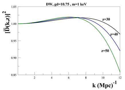
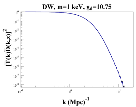
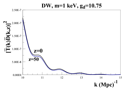
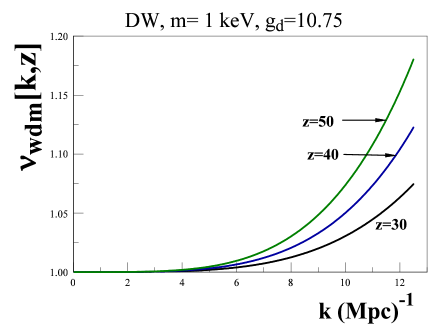
Figure 2: DW, $m=1~{}\mathrm{keV},g_{d}=10.75$: upper left panel $\overline{D}[k,z]$ and $[\overline{T}(k)\overline{D}(k,z)]^{2}$, lower panel: small scale region of $[\overline{T}(k)\overline{D}(k,z)]^{2}$ and $\mathcal{V}_{wdm}[k,z]$ all for $z=30,40,50$.

(BD) sterile neutrinos:

Sterile neutrinos produced by the decay of scalar or vector bosons at the electroweak scaleboysnudm ; jun are colder for two reasons, i) their decoupling occurs when $g_{d}\sim 100$ and they do not reheat when the entropy from other degrees of freedom is given off to the thermal plasma, ii) their distribution function (IV.2) is more enhanced at small momentum thereby yielding smaller velocity dispersion. For this species

$$\overline{y^{2}}=8.509~{}~{};~{}~{}\beta_{2}=2.890~{}~{};~{}~{}k_{fs}=14.107\,\Big{(}\frac{m}{\mathrm{keV}}\Big{)}\,\Big{(}\frac{g_{d}}{100}\Big{)}^{\frac{1}{3}}\,\Big{(}\mathrm{Mpc}\Big{)}^{-1}$$ (IV.4)

This case is displayed in fig.(3): the fig. for $[\overline{D}[k,z]]^{2}$ for $g_{d}=100$ (corresponding to freeze-out at the electroweak scale) also shows the crossover from an early enhancement as a consequence of free streaming to a later suppression of the power spectrum as a consequence of the extra contribution to free streaming from peculiar velocity at small scales. For $m=1\,\mathrm{keV}$ (the value used in the figure) $k_{fs}=14.107\,(\mathrm{Mpc})^{-1}$, and the figure clearly shows that, again, the crossover from enhancement to suppression occurs at $k\approx 1-2\,k_{fs}$ for $30\leq z\leq 50$ . The corrections from $\overline{D}[k,z]$ are not resolved in the log-log scale of the power spectrum, however a linear-linear display of the region $k\gtrsim 2\,k_{fs}$ reveals the $10-15\,\%$ suppression of the power spectrum. In this region the figure displays a hint of the (WDM) acoustic oscillations discussed in ref.smallscale . As discussed in ref.smallscale the smaller amplitude of the (WDM) acoustic oscillations as compared to the (DW) case are a reflection of the fact that (BD) sterile neutrinos are colder as explained above.

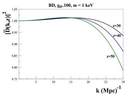
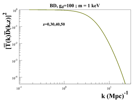
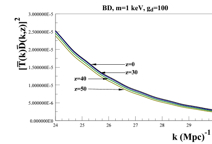
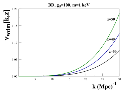
Figure 3: BD, $m=1~{}\mathrm{keV},g_{d}=100$: upper left panel $\overline{D}[k,z]$ and $[\overline{T}(k)\overline{D}(k,z)]^{2}$, lower panel: small scale region of $[\overline{T}(k)\overline{D}(k,z)]^{2}$ and $\mathcal{V}_{wdm}[k,z]$ all for $z=30,40,50$.

In both these cases, we see that there is a suppression of the power spectrum for $z\sim 30-50$ in the small scale region $k\simeq(1-2)\,k_{fs}$ and an enhancement of the peculiar velocity in the same region, both effects are at the $10-15\%$ level and clearly correlated: the larger peculiar velocity adds to free streaming depressing the power spectrum. Although these effects are at the level of few percent, it is conceivable that they may be magnified by the inherent non-linearities in the process of gravitational collapse, perhaps leading to important consequences for galaxy formation in N-body simulations.

V Conclusions

Motivated by recent and forthcoming N-body simulations of galaxy formation in (WDM) scenarios, we set out to study the redshift corrections to the matter and peculiar velocity power spectra and corrections to the phase space density from gravitational perturbations in the region $30\leq z\leq 50$. This is the region in redshift where N-body simulations set up initial conditions and the dark energy component can be safely neglected.

Drawing from results in ref.smallscale , we implemented a perturbative expansion for the redshift and scale dependence of the distribution function, matter density perturbations and coarse grained phase space density valid for $z/z_{eq}\ll 1$ and a wide range of scales, up to leading logarithmic order in the scale factor.

We find that for (WDM) the redshift dependence is determined by $\beta_{2}$, the kurtosis of the unperturbed distribution function after freeze-out, with an enhancement of of the peculiar velocity power spectrum and autocorrelation function at larger redshift for $\beta_{2}>1$. This enhancement in the peculiar velocity hastens free streaming and leads to a further suppression of the matter power spectrum for $k>(1-2)\,k_{fs}$, where $k_{fs}$ is the free streaming wavevector. For (WDM) gravitational perturbations lead to a suppression of the statistical fluctuations of velocities when $\beta_{2}>5/3$.

We also study the linear corrections to the coarse grained phase space density introduced in refs.dalcanton1 ; hogan ; coldmatter ; darkmatter ; hectornorma ; boysnudm resulting from gravitational perturbations. We find that whereas these vanish for (CDM) resulting in a constant (coarse grained) phase space density, (WDM) perturbations lead to a logarithmic growth with scale factor as a consequence of the suppression of statistical fluctuations if $\beta_{2}>1.19$.

Two specific examples of (WDM) candidates are studied in detail: sterile neutrinos produced non-resonantly either via the Dodelson-Widrow mechanismdw or via the decay of scalar or vector bosons at the electroweak scaleboysnudm ; jun . In these cases we find that the corrections to the power spectra of matter and peculiar velocities are of order $10-15\,\%$ for scales $k\simeq(1-2)\,k_{fs}$ and redshifts $z\simeq 30-50$.

Impact on the bounds on the mass: The scale and redshift dependence of the power spectra are encoded in the effective matter and velocity power spectra $P_{\delta}(k)\overline{D}^{\,2}[k,z]~{};~{}P_{\delta}(k)\mathcal{V}[k,z]$ with $\overline{D}[k,z]~{};~{}\mathcal{V}[k,z]$ given by eqns. (II.52,III.12) respectively.

To assess the impact of the above results on the bounds on the mass of the (WDM) particle consider two N-body simulations with a particle of the same mass both setting up initial conditions at the same $z\simeq 30-50$, one with the matter and peculiar velocity power spectra at $z\sim 1$ and the other with the spectra corrected by the scale and redshift dependent factors obtained above. If $\beta_{2}>1$ the corrected matter power spectrum features the (WDM) suppression and the peculiar velocity power spectrum features the (WDM) enhancement for $k\gtrsim k_{fs}$ found above. These effects at small scales are akin to the suppression of density fluctuations and enhancement of velocity dispersion associated with a lighter particle for the un-corrected power spectra. This is because a lighter particle features a smaller $k_{fs}$ and a larger velocity dispersion. Therefore these corrections allow larger masses to describe the same large scale structure output from the N-body simulations as compared to the un-corrected power spectra. Thus one aspect of the corrections is to allow larger mass (WDM) particles, thereby relaxing the bound on the mass, at least for those models for which $\beta_{2}>1$. However, this is not all there is to the corrections, because the coarse-grained phase space density increases, which would correspond to a colder particle with smaller velocity dispersion. Thus the net effect of the corrections cannot be simply characterized as being described by an increase or decrease of the mass of the particle and ultimately must be understood via a full N-body simulation.

Although these corrections are relatively small, non-linearities arising from gravitational collapse may result in a substantial amplification of these effects, if this is the case, and only large scale N-body simulations with the corrected power spectra can assess this possibility, then it is conceivable (and expected) that the bounds on the mass of the (WDM) particle may need substantial revision.

The results obtained here suggest a breakdown of perturbation theory either at large redshift and or small scales $k\gg k_{fs}$, this is clearly an artifact of the expansion, the integral in (II.27) which yields the logarithmic contribution is bounded and well behaved both in the small scale and $u\rightarrow u_{NR}$ limitssmallscale . However a systematic study of smaller scales and or larger redshifts would require a full numerical solution of the integro-differential equation (II.27). If future N-body simulations find that the corrections obtained here do modify the dynamics of large scale structure formation in (WDM) models substantially, such a study may be worthy of consideration.

- (1) B. Moore et. al., Astrophys. J. Lett. 524, L19 (1999).
- (2) G. Kauffman, S. D. M. White, B. Guiderdoni, Mon. Not. Roy. Astron. Soc. 264, 201 (1993).
- (3) S. Ghigna et.al. Astrophys.J. 544,616 (2000).
- (4) A. Klypin et. al. Astrophys. J. 523, 32 (1999); Astrophys. J. 522, 82 (1999).
- (5) B. Willman et.al. Mon. Not. Roy. Astron. Soc. 353, 639 (2004).
- (6) J. F. Navarro, C. S. Frenk, S. White, Mon. Not. R. Astron. Soc. 462, 563 (1996).
- (7) J. Dubinski, R. Carlberg, Astrophys.J. 378, 496 (1991).
- (8) J. S. Bullock et.al., Mon.Not.Roy.Astron.Soc. 321, 559 (2001); A. R. Zentner, J. S. Bullock, Phys. Rev. D66, 043003 (2002); Astrophys. J. 598, 49 (2003).
- (9) J. Diemand et.al. Mon.Not.Roy.Astron.Soc. 364, 665 (2005).
- (10) J. J. Dalcanton, C. J. Hogan, Astrophys. J. 561, 35 (2001).
- (11) F. C. van den Bosch, R. A. Swaters, Mon. Not. Roy. Astron. Soc. 325, 1017 (2001).
- (12) R. A.Swaters, et.al., Astrophys. J. 583, 732 (2003).
- (13) R. F.G. Wyse and G. Gilmore, arXiv:0708.1492; G. Gilmore et. al. arXiv:astro-ph/0703308; G. Gilmore et.al. arXiv:0804.1919 (astro-ph); G. Gilmore, arXiv:astro-ph/0703370.
- (14) G.Gentile et.al Astrophys. J. Lett. 634, L145 (2005); G. Gentile et.al., Mon. Not. Roy. Astron. Soc. 351, 903 (2004); V.G. J. De Blok et.al. Mon. Not. Roy. Astron. Soc. 340, 657 (2003), G. Gentile et.al.,arXiv:astro-ph/0701550; P. Salucci, A. Sinibaldi, Astron. Astrophys. 323, 1 (1997).
- (15) G. Battaglia et.al. arXiv:0802.4220.
- (16) W. J. G. de Blok, arXiv:0910.3538.
- (17) See also: A. Kravstov, arXiv:0906.3295.
- (18) W.J.G. de Blok et.al., Ast.Jour. 136, 2648 (2008); Se-H. Oh et.al. arXiv: 1011.0899.
- (19) P. Salucci et al. MNRAS 378, 41 (2007); P. Salucci, arXiv:0707.4370.
- (20) B. Moore, et.al. Mon. Not. Roy. Astron. Soc. 310, 1147 (1999);
- (21) P. Bode, J. P. Ostriker, N. Turok, Astrophys. J 556, 93 (2001)
- (22) V. Avila-Reese et.al. Astrophys. J. 559, 516 (2001).
- (23) J. R. Bond, G. Efstathiou, J. Silk, Phys. Rev. Lett. 45, 1980 (1980).
- (24) A. V. Tikhonov, A. Klypin,MNRAS 395,1915 (2009).
- (25) A. V. Tikhonov, S. Gottlober, G. Yepes, Y. Hoffman, arXiv:0904.0175.
- (26) A. V. Maccio, F. Fontanot, arXiv:0910.2460.
- (27) U. Seljak et.al. Phys. Rev. Lett. 97, 191303 (2006); M. Viel et.al. Phys. Rev. Lett. 97 071301 (2006).
- (28) M. Viel et. al. , Phys.Rev.Lett. 100 (2008) 041304; A. Boyarsky et.al., JCAP 05, 012 (2009).
- (29) M. Viel, et. al. Phys. Rev. D71, 063534 (2005).
- (30) K. Abazajian, S. M. Koushiappas, Phys. Rev. D74, 023527 (2006).
- (31) A. V. Maccio, M. Miranda, MNRAS 382, 1225 (2007).
- (32) T. Sawala et.al, arXiv:1003.0671.
- (33) H. J. de Vega, N. Sanchez, Mon. Not. R. Astron. Soc. 404, 885 (2010); arXiv:0907.0006 .
- (34) H. J. de Vega, P. Salucci, N. G. Sanchez, arXiv:1004.1908 .
- (35) R. Kuzio de Naray et.al, ApJ, 710L, 161 (2010).
- (36) F. Villaescusa-Navarro, N. Dalal, arXiv: 1010.3008.
- (37) S. Tremaine, J.E. Gunn, Phys. Rev. Lett. 42, 407 (1979).
- (38) D. Lynden-Bell, Mon. Not. Roy. Astron. Soc. 136, 101 (1967), S. Tremaine, M. Henon, D. Lynden-Bell, Mon. Not. Roy. Astron. Soc. 219, 285 (1986).
- (39) W. Dehnen, Mon.Not.Roy.Astron.Soc. 360,869 (2005).
- (40) C. J. Hogan, J. J. Dalcanton, Phys. Rev. D62, 063511 (2000).
- (41) D. Boyanovsky, H. J. de Vega, N. Sanchez, Phys. Rev. D 77, 043518 (2008).
- (42) D. Boyanovsky, H. J. de Vega, N. Sanchez, Phys. Rev. D 78, 063546 (2008).
- (43) D. Boyanovsky, Phys.Rev.D78, 103505 (2008).
- (44) D. Boyanovsky, J. Wu, arXiv:1008.0992.
- (45) E. Komatsu et.al. (WMAP collaboration), arXiv:1001.4538
- (46) C.-P. Ma, E. Bertschinger, Astrophys. J. 455, 7 (1995).
- (47) S. Dodelson Modern Cosmology, (Academic Press, N.Y. 2003).
- (48) M. Giovannini, A Primer on the physics of the cosmic microwave background, (World Scientific, Singapore, 2008).
- (49) D. H. Lyth, A. R. Liddle, The primordial density perturbation (Cambridge University Press, Cambridge, UK, 2009).
- (50) S. Weinberg Cosmology, (Oxford University Press, Oxford, 2008).
- (51) R. Durrer, The cosmic microwave background, (Cambridge University Press, Cambridge, UK 2008).
- (52) H. Kodama, M. Sasaki, Int. J. Mod. Phys.A1,265 (1986).
- (53) P. Meszaros, Astr.Astroph. , 37,225 (1974)
- (54) E. J. Groth, P. J. E. Peebles, Astr.Astroph. , 41,143 (1975).
- (55) P. J. E. Peebles, The large scale structure of the Universe, (Princeton series in Physics, Princeton Univ. Press, Princeton, 1980).
- (56) S. Peirani, J.A. de Freitas Pacheco, astro-ph/0701292; S. Peirani et.al. Mon.Not.Roy.Astron.Soc. 367, 1011 (2006).
- (57) Y. Hoffman et.al., arXiv:0706.0006.
- (58) S. Dodelson, L. M. Widrow, Phys. Rev. Lett. 72, 17 (1994).
- (59) J. Wu, C.-M.Ho, D. Boyanovsky, Phys. Rev. D80, 103511 (2009).