Quantization via Mirror Symmetry

Abstract.

When combined with mirror symmetry, the $A$-model approach to quantization leads to a fairly simple and tractable problem. The most interesting part of the problem then becomes finding the mirror of the coisotropic brane. We illustrate how it can be addressed in a number of interesting examples related to representation theory and gauge theory, in which mirror geometry is naturally associated with the Langlands dual group. Hyperholomorphic sheaves and $(B,B,B)$ branes play an important role in the $B$-model approach to quantization.

1. Introduction

Anyone who is not shocked by quantum theory

has not understood a single word.

Niels Bohr

The quantization problem of a symplectic manifold $(M,\omega)$ can be approached via the topological $A$-model of $Y$, a complexification of $M$ [GW]. In this approach, the Hilbert space ${\mathcal{H}}$ obtained by quantization of $(M,\omega)$ is the space of open string states between two $A$-branes, ${\mathcal{B}}^{\prime}$ and ${\mathcal{B}}_{cc}$,

(1.1) $${\mathcal{H}}\;=\;{\rm space~{}of~{}}({\mathcal{B}}_{cc},{\mathcal{B}}^{\prime}){\rm~{}strings}\,,$$

where ${\mathcal{B}}^{\prime}$ is an ordinary Lagrangian $A$-brane, and ${\mathcal{B}}_{cc}$ is a space-filling coisotropic $A$-brane. More formally, we can write (1.1) as the space of morphisms

(1.2) $${\mathcal{H}}\;=\;{\rm Hom}({\mathcal{B}}_{cc},{\mathcal{B}}^{\prime})$$

between two objects, ${\mathcal{B}}_{cc}$ and ${\mathcal{B}}^{\prime}$, in the Fukaya category of $Y$.

In general, in a Fukaya category the space of morphisms between two Lagrangian objects, ${\mathcal{B}}_{1}$ and ${\mathcal{B}}_{2}$, is given by the symplectic Floer homology, $HF_{{\rm symp}}^{*}({\mathcal{B}}_{1},{\mathcal{B}}_{2})$. Therefore, if both of our objects in (1.2) were familiar Lagrangian objects, the space of morphisms ${\mathcal{H}}$ would be obtained by counting their intersection points and analyzing pseudo-holomorphic disks with boundary on ${\mathcal{B}}_{1}$ and ${\mathcal{B}}_{2}$.

However, our situation is more complicated and more interesting due to the fact that one of the objects, namely ${\mathcal{B}}_{cc}$, is coisotropic. As a result, the space of morphisms (1.2) is not “local” (in a sense that it does not localize to a set of points in $Y$) and, according to [GW], is the Hilbert space obtained by quantizing $(M,\omega)$. Put differently, the results of [AZ, GW] can be interpreted as a statement that the space of morphisms between two objects, at least one of which is coisotropic, is closely related to quantization.

More generally, the study of coisotropic branes and their role in the construction of the Fukaya category is an outstanding interesting problem. Although we will not try to solve it in the present paper, we will be able to gain some insights by using mirror symmetry.

The computation of the space of morphisms (1.2) can be simplified if the space $Y$ happens to admit additional structures. For example, if $Y$ is hyper-Kähler then it is often instructive to look at ${\mathcal{B}}_{cc}$ and ${\mathcal{B}}^{\prime}$ from the vantage point of all three complex structures, $I$, $J$, and $K=IJ$, as well as the corresponding symplectic structures $\omega_{I}$, $\omega_{J}$, and $\omega_{K}$. Even though originally we were interested in ${\mathcal{B}}_{cc}$ and ${\mathcal{B}}^{\prime}$ as objects in the Fukaya category often they can be defined as half-BPS boundary conditions in the ${\mathcal{N}}=(4,4)$ sigma-model of $Y$, which means that they are also $A$-branes for some other $A$-model of $Y$, and $B$-branes for a certain $B$-model of $Y$. In particular, the latter implies that (1.2) can be also computed in the $B$-model of $Y$:

(1.3) $${\mathcal{H}}\;=\;\operatorname{Ext}^{*}_{Y}({\mathcal{B}}_{cc},{\mathcal{B}}^{\prime})\,.$$

Another example of a useful structure is a Calabi-Yau structure. In such case, if $Y$ admits a Calabi-Yau metric, one can approach the computation of (1.2) in the mirror $B$-model:

(1.4) $${\mathcal{H}}\;=\;\operatorname{Ext}^{*}_{\widetilde{Y}}({\widetilde{\mathcal{B}}}_{cc},\widetilde{\mathcal{B}}^{\prime})\,,$$

where ${\widetilde{\mathcal{B}}}_{cc}$ is the mirror of ${\mathcal{B}}_{cc}$, and $\widetilde{\mathcal{B}}^{\prime}$ is the mirror of ${\mathcal{B}}^{\prime}$. As we explain below, the hyper-Kähler structure on $Y$ and mirror symmetry can both be very useful tools in understanding quantization via categories of $A$- and $B$-branes. However, combining these tools together can double their power!

We start our discussion in the next section with a friendly introduction to the quantization problem. Our goal is to explain why this problem is interesting and why it is hard. Along the way, we often illustrate the general ideas and key concepts with concrete and (hopefully) simple examples, many of which have applications to representation theory and gauge theory. After recalling the $A$-model approach to quantization in section 2.3, we reformulate the problem in the mirror $B$-model and illustrate it in a number of examples in section 3.

One of our examples is so rich and important that it deserves a separate section. Thus, in section 4 we apply the mirror approach to quantization of Chern-Simons gauge theory, where the classical phase space $M$ is the moduli space, ${\mathcal{M}}_{{\rm flat}}(G,C)$, of flat connections on a Riemann surface $C$. One interesting feature of this example is that, for a compact Lie group $G$, the coisotropic brane ${\mathcal{B}}_{cc}$ is defined only for a discrete set of symplectic structures on $Y$, indexed by an integer number $k$ called the “level.” Quantization of $M$ leads to a finite-dimensional Hilbert space ${\mathcal{H}}$, whose dimension is given by the celebrated Verlinde formula [V]. In general, the Verlinde formula has the following form:

(1.5) $$\dim{\mathcal{H}}\;=\;a_{n}k^{n}+a_{n-1}k^{n-1}+\ldots+a_{1}k+a_{0}\,,$$

where $a_{i}$ are rational numbers. One novelty of our approach is that it offers an interpretation of the coefficients $a_{i}$ in terms of branes on moduli spaces of Higgs bundles. The coefficients $a_{n},a_{n-1},\ldots$ determine the asymptotic behavior of this polynomial in the “classical” limit $\hbar=\frac{1}{k}\to 0$. Similarly, the coefficients $a_{0},a_{1},\ldots$ determine the behavior of the polynomial (1.5) in the opposite, “very quantum” regime $\hbar=\frac{1}{k}\to\infty$ which, as we explain in section 4, corresponds to the classical limit ${}^{L}{\hbar}=-\frac{1}{\hbar}\to 0$ of the mirror theory based on the Langlands dual group ${}^{L}\negthinspace G$.

As a result, the coefficients $a_{n},a_{n-1},\ldots$ have a simple interpretation (in terms of classical geometry of $Y$) and are easier to determine in the $A$-model based on the moduli space of Higgs bundles with the structure group $G$. On the other hand, the coefficients $a_{0},a_{1},\ldots$ have a simpler interpretation and are easier to determine in the dual $B$-model, based on the moduli space of Higgs bundles for the Langlands dual group ${}^{L}\negthinspace G$. In section 5, we present a derivation of the Verlinde formula using this approach in a concrete example.

2. Quantization is an art

Very interesting theory — it makes no sense at all.

Groucho Marx (about Quantum Mechanics)

The basic problem of quantization begins with a symplectic manifold $M$, called a classical “phase space,” equipped with a symplectic form $\omega$. By quantizing $(M,\omega)$ one can mean a number of different things, but usually one is asking for a machinery that allows to turn the following “classical” objects into their “quantum” analogs:

(2.1) $$\begin{array}[]{ccc}(M,\omega)&\rightsquigarrow&{\mathcal{H}}~{}(=\text{Hilbert space})\\ &&\raisebox{-2.84544pt}{\includegraphics[width=14.22636pt]{actsbelow}}\\ \text{alg. of functions on $M$}&\rightsquigarrow&\text{~{}~{}alg. ${\mathcal{A}}_{\hbar}$ of operators on ${\mathcal{H}}$}\\ f&\mapsto&{\mathcal{O}}_{f}:{\mathcal{H}}\to{\mathcal{H}\vspace{3mm}}\\ \text{Lagrangian submanifolds}&\rightsquigarrow&\text{vectors}\\ L\subset M&\mapsto&\psi\in{\mathcal{H}\vspace{3mm}}\\ \text{symplectomorphisms}&\rightsquigarrow&\text{automorphisms}\\ \text{of}~{}M&&\text{of}~{}{\mathcal{A}}_{\hbar}\vspace{1mm}\end{array}$$

There are various interrelations between the classical structures on the left-hand side of this list, which should be reflected in their quantum counterparts (the right-hand side). Moreover, depending on specific applications, one can put more items to this “wish list”; here we listed only the standard ones.

Since the only input data is $(M,\omega)$ it is not surprising that all of the items on the left-hand side of (2.1) are the standard gadgets in symplectic geometry. Therefore, quantization can be regarded as a program of constructing a “quantum version” of symplectic geometry.

Another area where the input data is a symplectic manifold is mirror symmetry. Much like the problem of quantization, it starts with a symplectic manifold and constructs the Gromov-Witten invariants, the Fuakaya category, and many other interesting invariants, some of which are even called “quantum” (e.g. quantum cohomology). Is there any relation between these two problems?

As we explain below, the answer is “yes” and the quantization problem can indeed be reformulated as a certain problem in mirror symmetry, however, not in the most naive and obvious way. In particular, the problem of quantizing a symplectic manifold $(M,\omega)$ can be directly related to a problem in the Fukaya category of another symplectic manifold, namely a complexification of $(M,\omega)$.

However, before we are ready to review the results of [GW] and formulate them in terms of mirror symmetry, we need to explain some of the delicate features of quantization and to introduce important examples. Since the real dimension of a symplectic manifold is always even, the simplest non-trivial example is either a 2-sphere, $M={\bf S}^{2}$, or a 2-dimensional plane, $M=\mathbb{R}^{2}$ (depending on whether we prefer compact or non-compact manifolds).

 Example. Quantization of $M={\bf S}^{2}$

One can represent $(M,\omega)$ as a unit sphere in a 3-dimensional space $\mathbb{R}^{3}$,

(2.2) $$x^{2}+y^{2}+z^{2}=1\,,$$

with a symplectic form

(2.3) $$\omega=\frac{1}{4\pi\hbar}\frac{dx\wedge dy}{z}\,.$$

While it may not be immediately obvious, the 2-form $\omega$ is invariant under the $SO(3)$ symmetry of eq. (2.2). Indeed, using a relation between the Cartesian coordinates $(x,y,z)$ and the spherical coordinates $(r,\theta,\varphi)$,

$$x = r\sin\theta\cos\varphi$$

$$y = r\sin\theta\sin\varphi$$

$$z = r\cos\theta$$

one can write (2.3) as a multiple of the standard volume form on a 2-sphere, $\omega=\frac{1}{4\pi\hbar}\sin\theta~{}d\theta\wedge d\varphi$. According to textbooks, quantization of $(M,\omega)$ gives a finite-dimensional Hilbert space ${\mathcal{H}}$, such that

(2.4) $$\dim{\mathcal{H}}=\int_{M}\omega=\frac{1}{\hbar}\,.$$

In particular, $\dim{\mathcal{H}}$ must be an integer and this shows that quantization of $(M,\omega)$ is possible only for discrete values of the parameter $\hbar$:

(2.5) $$\hbar^{-1}\;\in\;\mathbb{Z}\,.$$

 

In what follows, we consider a variety of interesting examples in which symplectic manifolds come from problems in representation theory on one hand, and from gauge theory and low-dimensional topology, on the other. These examples provide an excellent laboratory for the quantization problem.

As a necessary preliminary to both groups of examples, we introduce the following notations that will be used throughout the rest of this paper:

• $=~{}$ (simple) compact Lie group,

• $=~{}$ complexification of $G$,

• $=~{}$ real form of $G_{\mathbb{C}}$.

In particular, $G_{\mathbb{R}}$ may be equal to $G$. For concreteness, one can keep in mind a simple example of $G=SU(2)$, for which $G_{\mathbb{C}}=SL(2,\mathbb{C})$ and $G_{\mathbb{R}}$ can be either a compact real form $SU(2)$ (equal to $G$) or a split real form $SL(2,\mathbb{R})$.

Now, we can proceed to some interesting examples of symplectic manifolds. As we mentioned earlier, a large supply comes from representation theory. Let ${\mathcal{O}}_{\mathbb{R}}(\lambda)=G_{\mathbb{R}}\cdot\lambda$ be a coadjoint orbit through an element $\lambda\in\mathfrak{g}_{\mathbb{R}}^{*}$, where $\mathfrak{g}_{\mathbb{R}}={\rm Lie}(G_{\mathbb{R}})$ and $\mathfrak{g}_{\mathbb{R}}^{*}$ denotes its dual. To avoid cluttering, we often write ${\mathcal{O}}_{\mathbb{R}}(\lambda)$ simply as ${\mathcal{O}}_{\mathbb{R}}$. Then, any such coadjoint orbit is an example of a symplectic manifold [K1]. Indeed, $M={\mathcal{O}}_{\mathbb{R}}$ comes equipped with the Kostant-Kirillov-Souriau Poisson structure / symplectic structure that can be written explicitly

(2.6) $$\pi=\omega^{-1}=f^{ij}_{k}X^{k}\partial_{i}\wedge\partial_{j}$$

in terms of the structure constants $f^{ij}_{k}$ of $\mathfrak{g}_{\mathbb{R}}$.

 Example. $G_{\mathbb{R}}=SU(2)$

In this case, the stabilizer of a generic element $\lambda\in\mathfrak{g}_{\mathbb{R}}^{*}$ is a one-dimensional (abelian) subgroup of $G_{\mathbb{R}}=SU(2)$, so that ${\mathcal{O}}_{\mathbb{R}}=SU(2)/U(1)\cong{\bf S}^{2}$ is simply a 2-sphere, as in our previous example. Moreover, since the structure constants are given by the totally antisymmetric symbol, $f^{ijk}=\epsilon^{ijk}$, the Kirillov-Kostant symplectic form (2.6) coincides with the one written in (2.3) if we identify the three-dimensional space $\mathbb{R}^{3}$ parametrized by $(x,y,z)$ with (the dual of) the Lie algebra $\mathfrak{g}_{\mathbb{R}}=\mathfrak{su}(2)$. Therefore, these two examples are in fact identical.  

Since the classical phase space $M={\mathcal{O}}_{\mathbb{R}}$ enjoys the action of the symmetry group $G_{\mathbb{R}}$, this property should be reflected in its quantum counterpart. Namely, the Hilbert space ${\mathcal{H}}$ obtained from quantization of $(M,\omega)$ should carry a unitary representation of the group $G_{\mathbb{R}}$. This is the basic idea of the orbit method.

However, there have always been some puzzles with this approach to representations of real groups, which can serve us as important lessons for understanding the quantization problem:

• there exist unitary representations that don’t appear to correspond to orbits;

• conversely, there are real orbits that don’t seem to correspond to unitary representations.

An example of the first problem occurs even in the basic case of the real group $G_{\mathbb{R}}=SL(2,\mathbb{R})$ and the complementary series representations. To illustrate the second phenomenon, one can take $G_{\mathbb{R}}$ to be a real group of Cartan type $B_{N}$, i.e. $G_{\mathbb{R}}=SO(p,q)$ with $p+q=2N+1$. The minimal orbit ${\mathcal{O}}_{{\rm min}}$ of $B_{N}$ is a nice symplectic manifold of (real) dimension $4N-4$, for any values of $p$ and $q$. On the other hand, the corresponding representation of $SO(p,q)$ exists only if $p\leq 3$ or $q\leq 3$, and does not exist if $p,q\geq 4$. This curious observation [Vo] follows from a rather lengthy algebra and cries out for a simple geometric interpretation!

In other words, it would be desirable to have a set of simple topological and/or geometric criteria that, starting with a symplectic manifold $(M,\omega)$, would tell us beforehand whether it should be quantizable or not. Such criteria naturally emerge in the brane quantization approach [GW] where both of the aforementioned issues can be resolved at the cost of of replacing classical geometric objects (namely, coadjoint orbits) with their “stringy” analogs (branes). In particular, in the case of $B_{N}$ one finds that, while the minimal orbit exists for any values of $p$ and $q$, the corresponding brane exists only if $p\leq 3$ or $q\leq 3$. (In general, the condition is that the second Stieffel-Whitney class $w_{2}(M)\in H^{2}(M;\mathbb{Z}_{2})$ must be a mod 2 reduction of a torsion class in the integral cohomology of $M$.)

Our second class of examples (in fact, also related to representation theory) comes from gauge theory and low-dimensional topology. Namely, let us consider Chern-Simons gauge theory with a real gauge group $G_{\mathbb{R}}$ (that may be compact or not). The key ingredients in any gauge theory include a gauge connection $A$ and the partial differential equations (PDEs) that it obeys. In the context of Chern-Simons theory, the relevant equations are the flatness equations and, according to Atiyah and Bott [AB], the moduli space of flat connections on a compact oriented 2-manifold is a finite-dimensional symplectic manifold (possibly singular).

Specifically, let $A$ be a connection on a $G_{\mathbb{R}}$ bundle $E\to C$ over a genus-$g$ Riemann surface $C$. Then, the moduli space of flat connections on $C$, $M={\mathcal{M}}_{{\rm flat}}(G_{\mathbb{R}},C)$, is the space of homomorphisms $\pi_{1}(C)\to G_{\mathbb{R}}$ modulo gauge transformations (i.e. modulo conjugation). In order to get a better idea of what this space looks like, we can describe it more concretely by introducing $G_{\mathbb{R}}$-valued holonomies, $A_{i}$, $B_{j}$, $i,j=1,\ldots,g$ of the gauge connection over a complete basis of $A$-cycles and $B$-cycles. Then, the space $M={\mathcal{M}}_{{\rm flat}}(G_{\mathbb{R}},C)$ can be viewed as a space of solutions to the equation

(2.7) $$A_{1}B_{1}A_{1}^{-1}B_{1}^{-1}~{}\ldots~{}A_{g}B_{g}A_{g}^{-1}B_{g}^{-1}={\bf 1}$$

modulo conjugation by $G_{\mathbb{R}}$. In total, the group elements $A_{i}$ and $B_{j}$ contain $2g\dim G_{\mathbb{R}}$ real parameters, so that generically, for $g>1$, after imposing the equation (2.7) and dividing by conjugation we obtain a space of real dimension $\dim M=2(g-1)\dim G_{\mathbb{R}}$.

The space $M={\mathcal{M}}_{{\rm flat}}(G_{\mathbb{R}},C)$ comes equipped with a natural symplectic form

(2.8) $$\omega=\frac{1}{4\pi^{2}\hbar}\int_{C}\operatorname{Tr}\delta A\wedge\delta A\,,$$

where the parameter $k:=\frac{1}{\hbar}$ is called the “level.” What does one find in quantizing $(M,\omega)$? In particular, what is the Hilbert space ${\mathcal{H}}$? What is the dimension of ${\mathcal{H}}$?

The answer to these questions turns out to be surprisingly rich, and depends in a crucial way on the choice of $G_{\mathbb{R}}$. If $G_{\mathbb{R}}=G$ is compact, the space $(M,\omega)$ is quantizable only for integer values of the level,

(2.9) $$k=\frac{1}{\hbar}\;\in\;\mathbb{Z}$$

In this case, the corresponding Hilbert space ${\mathcal{H}}$ is finite-dimensional, and $\dim{\mathcal{H}}$ is a polynomial in $k$, whose leading coefficient equals the volume of $M$ with respect to the symplectic form $\omega$, cf. (2.4),

(2.10) $$\dim{\mathcal{H}}=\int_{M}\frac{\omega^{n}}{n!}+\ldots\,,$$

where $\dim M=2n$. Specifically, ${\mathcal{H}}$ is the space of conformal blocks in the WZW model at level $k$, and the dimension of ${\mathcal{H}}$ is given by the celebrated Verlinde formula [V] (see [B] for a nice review). This is only the beginning of a very beautiful story that leads to the Witten-Reshetikhin-Turaev invariants of knots and 3-manifolds.

 Example. $G=SU(N)$

The dimension of ${\mathcal{H}}$ is given by the following explicit formula:

(2.11) $$\dim{\mathcal{H}}=\left(\frac{N}{k+N}\right)^{g}~{}\sum_{{S\amalg T=[1,k+N]\atop|S|=N}}~{}\prod_{{s\in S\atop t\in T}}|2\sin\pi\frac{s-t}{k+N}|^{g-1}\,.$$

Notice, from this formula it is completely non-obvious that $\dim{\mathcal{H}}$ is a polynomial in $k$, e.g. for $G=SU(2)$ and $g=2$ it gives:

(2.12) $$\dim{\mathcal{H}}=\frac{1}{6}k^{3}+k^{2}+\frac{11}{6}k+1\,.$$

Here, the leading term equals ${\rm Vol}(M)={\rm Vol}({\mathbb{C}}{\mathbf{P}}^{3})=\frac{1}{6}k^{3}$, in agreement with (2.10) and the well-known fact $M\cong{\mathbb{C}}{\mathbf{P}}^{3}$ for $G=SU(2)$ and $g=2$.  

The story is very different if $G_{\mathbb{R}}$ is non-compact. In this case, the Hilbert space ${\mathcal{H}}$ is infinite-dimensional, and much less is known about the corresponding quantum group invariants. In particular, the analogs of the Witten-Reshetikhin-Turaev invariants are still waiting to be discovered.

The two general classes of examples considered here — based on coadjoint orbits and moduli spaces of flat connections — are actually much closer related than one might think. Indeed, a coadjoint orbit ${\mathcal{O}}_{\mathbb{R}}$ (more precisely, the corresponding conjugacy class $\mathfrak{C}_{\mathbb{R}}\subset G_{\mathbb{R}}$) naturally appears as a “local model” for ${\mathcal{M}}_{{\rm flat}}(G_{\mathbb{R}},C)$ if we take $C$ to be a punctured disc, see e.g. [GW1]. In fact, these two classes of examples can be naturally combined in a larger family by picking a set of “marked points” $p_{i}$, $i=1,\ldots,h$ on the Riemann surface $C$ and requiring the gauge field $A$ to have certain singularities at the points $p_{i}$. Equivalently, one can remove the points $p_{i}$ and study Riemann surfaces with punctures (or boundary components).

For ease of exposition, let us consider a Riemann surface with only one puncture $p\in C$, around which the gauge field has a holonomy

(2.13) $$V={\rm Hol}_{p}(A)\;\in\;\mathfrak{C}_{\mathbb{R}}\,,$$

that takes values in a prescribed conjugacy class $\mathfrak{C}_{\mathbb{R}}\subset G_{\mathbb{R}}$. In this way, associating a conjugacy class to a puncture, we obtain the moduli space $M={\mathcal{M}}_{{\rm flat}}(G_{\mathbb{R}},C;\mathfrak{C}_{\mathbb{R}})$ of flat connections on $C\setminus p$. As in (2.7), this moduli space can be described rather explicitly as a space of solutions to the equation

(2.14) $$A_{1}B_{1}A_{1}^{-1}B_{1}^{-1}~{}\ldots~{}A_{g}B_{g}A_{g}^{-1}B_{g}^{-1}=V\,,$$

modulo conjugation by $G_{\mathbb{R}}$.

The moduli space $M={\mathcal{M}}_{{\rm flat}}(G_{\mathbb{R}},C;\mathfrak{C}_{\mathbb{R}})$ is a symplectic manifold, with the symplectic form $\omega$ given by the general formula (2.8). At least when $V$ is sufficiently close to ${\bf 1}$, it has the structure of a symplectic fibration

(2.15) $$\begin{matrix}\mathfrak{C}_{\mathbb{R}}&\to&{\mathcal{M}}_{{\rm flat}}(G_{\mathbb{R}},C;\mathfrak{C}_{\mathbb{R}})\\ &&\downarrow\!\imath\\ &&~{}{\mathcal{M}}_{{\rm flat}}(G_{\mathbb{R}},C)\end{matrix}$$

Furthermore, the symplectic form on ${\mathcal{M}}_{{\rm flat}}(G_{\mathbb{R}},C;\mathfrak{C}_{\mathbb{R}})$ is

(2.16) $$\omega=\imath^{*}\omega_{{\mathcal{M}}}+\omega_{\mathfrak{C}}\,,$$

where $\omega_{{\mathcal{M}}}$ is the symplectic form on ${\mathcal{M}}_{{\rm flat}}(G_{\mathbb{R}},C)$ and $\omega_{\mathfrak{C}}$ restricts to the Kostant-Kirillov-Souriau symplectic form (2.6) on each fiber of the symplectic fibration (2.15).

 Example. $G=SU(2)$

Unitary irreducible representations of $G=SU(2)$ can be labeled either by the highest weight $\lambda\in\mathbb{Z}_{\geq 0}$ or, equivalently, by the dimension $d=\lambda+1$. In the physics literature, a representation $R_{\lambda}=S^{\lambda}\mathbb{C}^{2}$ is often called the spin-$j$ representation, where $j=\lambda/2$. As in (2.13), we can associate a representation $R_{\lambda}$ to a marked point $p\in C$ by making a puncture, such that on a small loop around $p$ the gauge field has a holonomy conjugate to:

(2.17) $$V\;=\;\exp 2\pi i\begin{pmatrix}\alpha&0\\ 0&-\alpha\end{pmatrix}\,,$$

with $\alpha=\frac{\lambda}{2k}$. Then, for a Riemann surface of genus $g$ with $h$ punctures, the Verlinde formula is

(2.18) $$\dim{\mathcal{H}}\;=\;\left(\frac{k+2}{2}\right)^{g-1}~{}\sum_{j=1}^{k+1}\left(\sin\frac{\pi j}{k+2}\right)^{2-2g-h}\prod_{i=1}^{h}\sin\frac{\pi j(\lambda_{i}+1)}{k+2}\,.$$

Believe it or not, this is an integer!  

Now, once we introduced a good supply of interesting symplectic manifolds, we shall return to our original problem of quantization of $(M,\omega)$. The quantization problem can be approached in many different ways. Each approach has its advantages and disadvantages, but in the end all methods are expected to yield the same result. Below we give a brief overview of various methods, quickly specializing to the brane quantization approach that will be used in the rest of this paper.

2.1. Geometric quantization

In geometric quantization [K2, S], in order to produce the desired items on the right-hand side of (2.1) one first needs to introduce some extra data that is not supplied with the symplectic manifold $(M,\omega)$. Then, of course, one needs to show that the result is, in a suitable sense, independent on these auxiliary choices. (This last step turns out to be the most difficult one almost in every approach to quantization.)

The first piece of extra data — which one needs to introduce not only in geometric quantization, but more or less in any approach to quantization — is a choice of line bundle, ${\mathcal{L}}\to M$, called the “prequantum line bundle” with a unitary connection of curvature $\omega$. Note, a prequantum line bundle ${\mathcal{L}}\to M$ only exists for

(2.19) $$[\omega]\in H^{2}(M;\mathbb{Z})\,,$$

which can lead to a quantization of $\hbar^{-1}$ (i.e. a restriction of $\hbar$ to a discrete set of values in $\mathbb{C}^{*}$). In fact, we already saw this phenomenon in our examples in (2.5) and (2.9).

The second choice of extra data is more delicate: it is a choice of polarization that, on local charts, corresponds to representing $M$ as a cotangent bundle $T^{*}U$. It is this second step where geometric quantization faces serious difficulties. Even if one can locally represent $M\simeq T^{*}U$ in every chart, such choices may not agree globally. Moreover, showing that the answer is independent of such choices becomes a rather difficult task.

2.2. Deformation quantization

Deformation quantization involves no auxiliary choices [BFFLS]. However, it is not a quantization in the sense of (2.1). Indeed, it does not construct the Hilbert space ${\mathcal{H}}$ and gives only a formal deformation of the ring of functions on $M$. In deformation quantization, there is no quantization condition on the parameter $\hbar$.

2.3. Brane quantization

As in other quantization methods, the approach of [GW] starts with a number of auxiliary choices that we summarize below:

• $Y=$ complexification of $M$, i.e. a complex manifold equipped with a complex structure that we shall call $J$ and an antiholomorphic involution $\tau:Y\to Y$, such that $\tau^{*}J=-J$ and $M$ is contained in the fixed point set of $\tau$,

• $\Omega=$ (non-degenerate) holomorphic 2-form, such that $\tau^{*}\Omega=\overline{\Omega}$ and

  $$\Omega|_{M}=\omega\,,$$

• ${\mathcal{L}}\to Y$ unitary line bundle (extending the “prequantum line bundle” ${\mathcal{L}}\to M$) with a connection of curvature ${\rm Re}\,\Omega$.

Of course, these data need to be consistent. For example, we need to ask for $\tau$ to lift to an action on ${\mathcal{L}}\to Y$, such that $\tau|_{M}={\rm id}$, etc.

To summarize, the basic idea is to pass from the original symplectic manifold $(M,\omega)$ and the prequantum line bundle ${\mathcal{L}}$ (that we often regard as a part of the initial data) to the complexification $(Y,\Omega)$ and ${\mathcal{L}}$. Then, the problem of quantizing $(M,\omega)$ can be formulated as a problem in the $A$-model / Fukaya category of $Y$ with symplectic structure

(2.20) $$\omega_{Y}=-{\rm Im}\,\Omega\,.$$

Note, the symplectic structure $\omega_{Y}$ is not a part of the original data, and appears only after we complexify the original phase space $M$.

Before we explain how all the desired items on the right-hand side of (2.1) can be produced in the $A$-model of $(Y,\omega_{Y})$, it is important to emphasize that in this approach to quantization the focus shifts from $M$ to $Y$, so that $Y$ takes the center of the stage. Then, from the vantage point of $Y$ it may be natural to consider close cousins of the original quantization problem suggested by the analysis of the $A$-model / Fukaya category of $Y$. For example, one can reduce the list of the auxiliary choices (see above) by omitting the involution $\tau$, which is needed only for unitarity. If one does not require this extra structure (namely, the Hermitian inner product on ${\mathcal{H}}$), then it suffices to introduce the complex symplectic manifold $(Y,\Omega)$ with a line bundle ${\mathcal{L}}\to Y$, and no involution $\tau$. From these data alone one can construct a space ${\mathcal{H}}$ and an algebra ${\mathcal{A}}_{\hbar}$ that acts on it. Later we consider examples of such situations related to representations theory.

We shall illustrate this approach to “quantization via complexification” in a variety of examples introduced earlier in this section; in particular, we apply it to $M={\mathcal{O}}_{\mathbb{R}}$ and $M={\mathcal{M}}_{{\rm flat}}(G_{\mathbb{R}},C)$. Although these examples have a very different flavor and come from completely different areas of physics and mathematics, they are closely related to representation theory of real groups and, at the most basic level, the complexification of $M$ can be understood as passing from a real group $G_{\mathbb{R}}$ to its complexification $G_{\mathbb{C}}$.

 Example. Quantization of $M={\mathcal{O}}_{\mathbb{R}}$

A coadjoint orbit ${\mathcal{O}}_{\mathbb{R}}$ of a real group $G_{\mathbb{R}}$ admits an obvious complexification, namely a complex coadjoint orbit of $G_{\mathbb{C}}$:

(2.21) $$Y={\mathcal{O}}_{\mathbb{C}}\,.$$

For example, the real coadjoint orbit (2.2) of $G_{\mathbb{R}}=SU(2)$ has a complexification $Y={\mathcal{O}}_{\mathbb{C}}$ described by the same equation $x^{2}+y^{2}+z^{2}=1$, where $x$, $y$, and $z$ are now complex variables. Moreover, eq. (2.3) written in terms of $(x,y,z)\in\mathbb{C}^{3}$ defines a holomorphic symplectic form $\Omega$ on $Y$.  

Similarly, there is an obvious complexification of the moduli space of flat connections, ${\mathcal{M}}_{{\rm flat}}(G_{\mathbb{R}},C)$.

 Example. Quantization of $M={\mathcal{M}}_{{\rm flat}}(G_{\mathbb{R}},C)$

This symplectic manifold $M$ admits an obvious complexification:

(2.22) $$Y={\mathcal{M}}_{{\rm flat}}(G_{\mathbb{C}},C)\,,$$

the moduli space of flat $G_{\mathbb{C}}$ connections on $C$. Much like $M$ itself, the space $Y$ can be explicitly described as a space of $G_{\mathbb{C}}$-valued holonomies $A_{i}$ and $B_{j}$ that satisfy (2.7), modulo conjugation by $G_{\mathbb{C}}$. It comes equipped with a holomorphic symplectic form $\Omega$ which, in terms of the $\mathfrak{g}_{\mathbb{C}}$-valued gauge connection, has the familiar form (2.8).  

In these examples, it is easy to verify that the holomorphic symplectic form $\Omega$ restricts to $\omega$ on $M\subset Y$.

Now let us return to the quantization problem of $(M,\omega)$ and explain how the desired items on the right-hand side of (2.1) can be produced in the approach of [GW]. The Hilbert space ${\mathcal{H}}$ is constructed as the space of morphisms (space of open strings),

(2.23) $${\mathcal{H}}\;=\;{\rm Hom}({\mathcal{B}}_{cc},{\mathcal{B}}^{\prime})\,,$$

where ${\mathcal{B}}_{cc}$ and ${\mathcal{B}}^{\prime}$ are objects (branes) of the Fukaya category of $(Y,\omega_{Y})$.

In general, typical objects of the Fukaya category of $(Y,\omega_{Y})$ are Lagrangian submanifolds of $Y$ equipped with flat unitary vector bundles and, in our setup, ${\mathcal{B}}^{\prime}$ is exactly such an object. Specifically, we define ${\mathcal{B}}^{\prime}$ to be an $A$-brane supported on $M\subset Y$. Indeed, according to our definitions,

(2.24) $$\omega_{Y}|_{M}=0\,,$$

so that $M$ is a Lagrangian submanifold of $Y$ with respect to $\omega_{Y}$.

Less familiar examples of $A$-branes (objects of the Fukaya category) are coisotropic submanifolds of $(Y,\omega_{Y})$ equipped with non-flat vector bundles (a.k.a. Chan-Paton bundles) with unitary connection that obeys certain conditions [KO]. In the simplest case of rank-1 coisotropic objects supported on all of $Y$, the condition on the curvature 2-form $F$ is

(2.25) $$(\omega_{Y}^{-1}F)^{2}=-1\,.$$

In our approach to quantization, ${\mathcal{B}}_{cc}$ is an example of such object, namely the so-called canonical coisotropic brane associated to a complexification of $(M,\omega)$ in a canonical way [GW].

To summarize, after we choose a complexification of $(M,\omega)$ and the extension of the prequantum line bundle ${\mathcal{L}}$, we can define two canonical objects in the Fukaya category of $(Y,\omega_{Y})$:

• Lagrangian $A$-brane supported on $M\subset Y$
  

• coisotropic $A$-brane supported on $Y$ and endowed with a unitary line bundle ${\mathcal{L}}$ with a connection of curvature

  $$F={\rm Re}\,\Omega$$

In particular, it is easy to verify that, with our definition of $\omega_{Y}$, the curvature 2-form $F$ indeed obeys the required condition (2.25).

Given two objects ${\mathcal{B}}^{\prime}$ and ${\mathcal{B}}_{cc}$, it is natural to consider the spaces of morphisms (spaces of open strings) in the $A$-model of $(Y,\omega_{Y})$. As we already stated in (2.23), the space of $({\mathcal{B}}_{cc},{\mathcal{B}}^{\prime})$ strings gives the Hilbert space ${\mathcal{H}}$ associated with the quantization of $(M,\omega)$. Just like in other quantization methods, one needs to show that it is independent on the auxiliary choices (which, among other things, involve the choice of complex structure $J$ on $Y$), i.e. to construct a flat connection on the ${\mathcal{H}}$-bundle over the space of such choices. In a closely related context, this problem has been studied in the mathematical physics literature [CV, D], and leads to a beautiful story that involves integrable systems and $tt^{*}$ equations.

 Example. Quantization of $M=T^{2}$

In this problem, $M=T^{2}$ admits an obvious complexification,

(2.26) $$Y\;\cong\;\mathbb{C}^{*}\times\mathbb{C}^{*}\,,$$

and the resulting Hilbert space ${\mathcal{H}}$ should not depend, among other things, on the choice of complex structure on $M=T^{2}$. If we denote by $t\in{\mathcal{T}}$ the corresponding complex structure parameter, then the states in ${\mathcal{H}}$ are simply theta functions of order $k$,

(2.27) $$\vartheta_{r}(z;t)=\sum_{n=-\infty}^{\infty}\exp\left(\frac{\pi it}{k}(kn+r)^{2}+2\pi i(kn+r)z\right)\quad\quad r\in\mathbb{Z}/k\mathbb{Z}\,,$$

where $k:=\dim{\mathcal{H}}=\frac{1}{\hbar}$, cf. (2.9). It is easy to see from (2.27) that $\vartheta_{r}(z;t)$ are quasi-periodic,

$$\vartheta_{r}(z+a+bt;t)\;=\;\exp\left(-\pi ikb^{2}t-2\pi ikbz\right)\vartheta_{r}(z;t)\quad\quad\quad a,b\in\mathbb{Z}$$

and obey the heat equation

(2.28) $$\left({\partial\over\partial t}-{\hbar\over 4\pi i}\;{\partial^{2}\over\partial z^{2}}\right)\vartheta_{r}(z;t)=0\,,$$

which gives a connection on a bundle ${\mathcal{H}}\to{\mathcal{T}}$. This example will be approached from a different viewpoint in section 3.2.  

Furthermore, in brane quantization the involution $\tau$ leads to a Hermitian inner product on ${\mathcal{H}}$. It is not necessarily positive definite; a necessary condition is that $\tau$ fixes $M$ pointwise outside of a compact support. This slight generalization of the condition that $M$ belongs to the fixed point set of $\tau$ is important e.g. for constructing the complementary series representations, where $\tau$ acts non-trivially on $M$.

The space of $({\mathcal{B}}_{cc},{\mathcal{B}}_{cc})$ strings, on the other hand, gives an associative but non-commutative algebra,

(2.29) $${\mathcal{A}}_{\hbar}\;=\;{\rm Hom}({\mathcal{B}}_{cc},{\mathcal{B}}_{cc})\,.$$

Note, this algebra depends only on $(Y,\Omega)$ and not on $M$. (In our examples, it means that the same algebra ${\mathcal{A}}_{\hbar}$ acts on Hilbert spaces obtained in quantization of $M={\mathcal{M}}_{{\rm flat}}(G_{\mathbb{R}},C)$ for different real forms $G_{\mathbb{R}}$ of $G_{\mathbb{C}}$, and similarly for $M={\mathcal{O}}_{\mathbb{R}}$.) In fact, we can think of the algebra ${\mathcal{A}}_{\hbar}$ as arising from the deformation quantization of $Y$.

The path integral of the quantum mechanics on $M$ also has an elegant realization in the $A$-model approach, see [W3] for details.

2.4. When does quantization exist?

While highly desirable, a complete set of geometric criteria that determine which symplectic manifolds are quantizable (and which are not) is not known at present. Most likely, such criteria should include the condition (2.19) that controls the existence of the prequantum line bundle ${\mathcal{L}}$ (and sometimes leads to a quantization of $\hbar$). However, this condition alone is clearly not enough, and — even as some of our examples suggest — there should be further criteria which determine whether $(M,\omega)$ is quantizable or not.

From the viewpoint of brane quantization, $(M,\omega)$ is expected to be quantizable whenever it admits a complexification, such that $(Y,\omega_{Y})$ has a “good” $A$-model / Fukaya category. A precise necessary condition for this is not known (in part, since the present understanding of the Fukaya category is incomplete). A sufficient condition, though, is that $(Y,\omega_{Y})$ admits a complete Calabi-Yau metric $g$, for which $\omega_{Y}$ is a Kähler form, i.e. $K=g^{-1}\omega_{Y}$ is an integrable complex structure. One indication that such criteria are on a right track is that, in deformation quantization, one encounters similar conditions that tell us whether ${\mathcal{A}}_{\hbar}$ is an actual deformation of the algebra of holomorphic functions on $(Y,\Omega)$, with a complex parameter $\hbar$ (not just a formal variable).

 Example. Quantization of $M={\bf S}^{2}$

In (2.2) we represented ${\bf S}^{2}$ as a unit sphere in $\mathbb{R}^{3}$. Its complexification,

(2.30) $$x^{2}+y^{2}+z^{2}=1\,,\qquad\qquad(x,y,z)\in\mathbb{C}^{3}$$

admits a complete Calabi-Yau metric (the Eguchi-Hanson metric) and a deformation of the ring of functions with a complex parameter $\hbar$ (not just a formal deformation). Both of these properties fail for a complex surface,

(2.31) $$x^{4}+y^{4}+z^{4}=1\,,\qquad\qquad(x,y,z)\in\mathbb{C}^{3}$$

that can be viewed as an alternative complexification of $M={\bf S}^{2}$.  

Besides the requirement for $(Y,\omega_{Y})$ to have a good $A$-model / Fukaya category, one needs ${\mathcal{B}}^{\prime}$ and ${\mathcal{B}}_{cc}$ to exist in order to solve the original quantization problem, i.e. to compute the spaces of morphisms (2.23) and (2.29). Fortunately, the existence of ${\mathcal{B}}^{\prime}$ and ${\mathcal{B}}_{cc}$ can be expressed in terms of concrete geometric criteria, which can be useful even in other quantization methods. Specifically, the brane ${\mathcal{B}}^{\prime}$ supported on $M$ exists whenever $M$ admits a flat Spin^c structure, and the brane ${\mathcal{B}}_{cc}$ exists whenever $[{\rm Re}\,\Omega]\in H^{2}(Y;\mathbb{Z})$, cf. (2.19).

3. $B$-model approach to quantization

Gott würfelt nicht!

Albert Einstein

In section 2.3 we reviewed the $A$-model approach to quantization [GW], where to a classical symplectic manifold $(M,\omega)$ one associates a Fukaya category of $A$-branes and the quantization (2.1) is achieved by studying the space of morphisms between two branes ${\mathcal{B}}_{cc}$ and ${\mathcal{B}}^{\prime}$. It is important to emphasize, however, that the Fukaya category in question is not that of the original symplectic manifold $(M,\omega)$. Rather, it is the Fukaya category of $Y$, a complexification of $M$, considered with a new symplectic form (2.20) that didn’t exist prior to complexification.

Another area of physics $\&$ mathematics where Fukaya categories are of major importance is mirror symmetry. In general, mirror symmetry relates the $A$-model of a symplectic manifold $Y$ to the $B$-model of a complex manifold $\widetilde{Y}$, called the mirror of $Y$. In mirror symmetry, however, the Fukaya category and $A$-model are usually considered to be the ‘difficult’ side of the correspondence, and it is often convenient to use mirror symmetry to map the problem to the simpler $B$-model side.

In our present context, this map is described by the homological mirror symmetry conjecture [K] that relates the derived Fukaya category of $Y$ and the (bounded) derived category of coherent sheaves on $\widetilde{Y}$. Specifically, the conjecture says that there exists a functor:

(3.1) $$\Phi_{{\rm mirror}}~{}:~{}~{}~{}{\rm{\bf Fuk}}(Y)\;\overset{\sim}{\longrightarrow}\;{\mathcal{D}}^{b}(\widetilde{Y})$$

such that it is the equivalence of triangulated categories. In the rest of this paper our goal will be to apply this map to the $A$-model of $(Y,\omega_{Y})$ described in section 2.3 and thereby to reformulate the quantization problem entirely in terms of the $B$-model.

In particular, mirror symmetry maps our $A$-branes ${\mathcal{B}}_{cc}$ and ${\mathcal{B}}^{\prime}$ to the dual $B$-branes:

(3.2) $$\widetilde{\mathcal{B}}^{\prime} = \Phi_{{\rm mirror}}({\mathcal{B}}^{\prime})$$

$${\widetilde{\mathcal{B}}}_{cc} = \Phi_{{\rm mirror}}({\mathcal{B}}_{cc})$$

whose geometry we wish to explore. Furthermore, mirror symmetry provides a dual description of the Hilbert space ${\mathcal{H}}$ and the algebra of quantum operators ${\mathcal{A}}_{\hbar}$ in terms of $\operatorname{Ext}$-groups of the dual objects $\widetilde{\mathcal{B}}^{\prime}$ and ${\widetilde{\mathcal{B}}}_{cc}$. For example, it identifies the space of morphisms (2.23) with

(3.3) $${\mathcal{H}}\;=\;\operatorname{Ext}^{*}_{\widetilde{Y}}({\widetilde{\mathcal{B}}}_{cc},\widetilde{\mathcal{B}}^{\prime})\,,$$

which can be analyzed using the standard tools of algebraic geometry. Thus, the Euler characteristic of (3.3) can be easily computed in the $B$-model with the help of the Grothendieck-Riemann-Roch theorem:

(3.4) $$\sum_{k}(-1)^{k}\dim\operatorname{Ext}^{k}_{\widetilde{Y}}({\widetilde{\mathcal{B}}}_{cc},\widetilde{\mathcal{B}}^{\prime})=\int_{\widetilde{Y}}\operatorname{ch}({\widetilde{\mathcal{B}}}_{cc})^{*}\wedge\operatorname{ch}(\widetilde{\mathcal{B}}^{\prime})\wedge{\rm Td}(\widetilde{Y})\,,$$

where $\operatorname{ch}(\widetilde{\mathcal{B}}^{\prime})$ (resp. $\operatorname{ch}({\widetilde{\mathcal{B}}}_{cc})$) is the Chern character of $\widetilde{\mathcal{B}}^{\prime}$ (resp. ${\widetilde{\mathcal{B}}}_{cc}$), ${\rm Td}(\widetilde{Y})$ is the Todd class of $\widetilde{Y}$, and $\omega^{*}$ denotes $(-1)^{p+1}\omega$ for any $2p$-form $\omega$. In applications, we will often use (3.4) to compute the dimension of the Hilbert space ${\mathcal{H}}$ (when $\dim{\mathcal{H}}<\infty$).

What are the mirror objects $\widetilde{\mathcal{B}}^{\prime}$ and ${\widetilde{\mathcal{B}}}_{cc}$? Does the mirror of the canonical coisotropic $A$-brane ${\mathcal{B}}_{cc}$ admit a ‘canonical’ definition in ${\mathcal{D}}^{b}(\widetilde{Y})$ (i.e. in the $B$-model of $\widetilde{Y}$)? What is the role of $\hbar$ in the $B$-model of $\widetilde{Y}$? In order to answer these and other questions about the $B$-model approach to quantization of $(M,\omega)$, it is useful to have a good geometric description of the mirror transform (3.1). One such description was proposed in 1996 by Strominger, Yau, and Zaslow [SYZ] (see also [BJSV]), who argued that mirror Calabi-Yau manifolds $Y$ and $\widetilde{Y}$ should fiber over the same base manifold ${B}$,

(3.5) $$\begin{array}[]{ccc}\!Y{}{}{}{}{}{}{}{}&&{}~{}~{}~{}~{}~{}~{}\widetilde{Y}\\ {}~{}~{}~{}~{}~{}~{}~{}{}_{\pi}\searrow&&\!\!\swarrow_{~{}\widetilde{\pi}}{}{}{}{}{}{}{}{}\\ &\!\!{B}&\end{array}$$

with generic fibers ${F}_{b}=\pi^{-1}(b)$ and $\widetilde{{F}}_{b}=\widetilde{\pi}^{-1}(b)$, $b\in{B}$, being dual tori, in the sense that ${F}_{b}=H^{1}(\widetilde{{F}}_{b},U(1))$ and $\widetilde{{F}}_{b}=H^{1}({F}_{b},U(1))$. Moreover, the fibers ${F}_{b}$ and $\widetilde{{F}}_{b}$ should be (special) Lagrangian submanifolds in $Y$ and $\widetilde{Y}$, respectively.

This way of looking at mirror symmetry can be very useful in understanding how the functor (3.1) acts on the $A$-branes ${\mathcal{B}}^{\prime}$ and ${\mathcal{B}}_{cc}$, which ultimately will lead us to a reformulation of the quantization problem in the mirror $B$-model. In particular, as we explain below, the fate of the coisotropic brane ${\mathcal{B}}_{cc}$ depends in a crucial way on whether the restriction of the symplectic form $F={\rm Re}\,\Omega$ on $Y$ to a generic fiber ${F}$ of the SYZ fibration (3.5) is trivial or not. When it is trivial, the coisotropic brane ${\mathcal{B}}_{cc}$ transforms under mirror symmetry to a brane ${\widetilde{\mathcal{B}}}_{cc}$ supported on a middle-dimensional submanifold of $\widetilde{Y}$, namely on a section of the dual SYZ fibration. (An example of such situation was considered e.g. in [KW].)

In contrast, when $F|_{{F}}$ is non-trivial, the story becomes more interesting and more complicated. In this case — which will be our subject here — mirror symmetry transforms the coisotropic brane ${\mathcal{B}}_{cc}$ into a $B$-brane ${\widetilde{\mathcal{B}}}_{cc}\in{\mathcal{D}}^{b}(\widetilde{Y})$ supported on all of $\widetilde{Y}$. Furthermore, in general ${\widetilde{\mathcal{B}}}_{cc}$ is a brane of a fairly high rank. In fact, using the SYZ picture (3.5) we conclude that the rank of ${\widetilde{\mathcal{B}}}_{cc}$ is given by

(3.6) $$\boxed{\phantom{\int}\operatorname{rank}({\widetilde{\mathcal{B}}}_{cc})\;=\;{\rm Vol}({F})\phantom{\int}}$$

where ${\rm Vol}({F})$ is the volume of the SYZ fiber ${F}$ computed with respect to the symplectic form $F={\rm Re}\,\Omega$ on $Y$,

(3.7) $$\operatorname{rank}({\widetilde{\mathcal{B}}}_{cc})\;=\;\int_{{F}}\frac{F^{n}}{n!}\,,$$

and $\dim_{\mathbb{R}}{F}=\dim_{\mathbb{C}}Y=2n$. (Remember, that in our context $Y$ is always a complex symplectic manifold.) Notice, the formula (3.6) also applies to the simpler case where $F|_{{F}}$ is trivial.

In what follows, we shall illustrate (3.6) in a variety of concrete examples. However, there is also a general argument based on (3.5) that we wish to sketch here since it will be very useful in later applications. In the $A$-model approach to quantization, ${\mathcal{B}}^{\prime}$ is a Lagrangian brane on $(Y,\omega_{Y})$. Since the fiber of the SYZ fibration (3.5) is Lagrangian with respect to $\omega_{Y}=-{\rm Im}\,\Omega$, we can choose ${\mathcal{B}}^{\prime}$ to be a Lagrangian brane supported on a generic fiber ${F}_{b}\subset Y$ and equipped with a unitary flat line bundle. In this simple warm-up example we know exactly what the dual object $\widetilde{\mathcal{B}}^{\prime}$ is. It is the skyscraper sheaf ${\mathcal{O}}_{p}\in{\mathcal{D}}^{b}(\widetilde{Y})$ of a point $p\in\widetilde{Y}$, such that $\widetilde{\pi}(p)=b$. For this reason, $\widetilde{\mathcal{B}}^{\prime}={\mathcal{O}}_{p}$ is often called a “zero-brane” or “D0-brane” on $\widetilde{Y}$. Summarizing,

(3.8) $$\Phi_{{\rm mirror}}~{}:~{}~{}~{}{\mathcal{B}}_{{F}}\;\rightarrow\;{\mathcal{B}}_{p}\,,$$

where we used slightly more intuitive notations ${\mathcal{B}}_{{F}}$ and ${\mathcal{B}}_{p}$ for this type of $A$-branes and $B$-branes, respectively.

In fact, the mirror pair of branes in (3.8) was an important part of the original motivation in [SYZ] that led to the proposed picture (3.5). One way to see that ${\mathcal{B}}_{{F}}$ and ${\mathcal{B}}_{p}$ should be mirror to each other is to consider their self-Homs. For a $B$-brane ${\mathcal{B}}_{p}={\mathcal{O}}_{p}$ on $\widetilde{Y}$, we have

(3.9) $$\operatorname{Ext}^{*}_{\widetilde{Y}}({\mathcal{B}}_{p},{\mathcal{B}}_{p})\cong\Lambda^{*}T_{p}\widetilde{Y}\cong H^{*}(T^{2n},\mathbb{C})\,.$$

As a gradede vector space, it is isomorphic to the Floer cohomology of ${F}\cong T^{2n}$, which describes the self-Homs of the $A$-brane ${\mathcal{B}}_{{F}}$:

(3.10) $$HF^{*}({\mathcal{B}}_{{F}},{\mathcal{B}}_{{F}})\cong H^{*}({F},\mathbb{C})\,,$$

hence, justifying (3.8).

Now, once we understand the duality (3.8) between branes ${\mathcal{B}}_{{F}}$ and ${\mathcal{B}}_{p}$, we can use it to “probe” the geometry of ${\widetilde{\mathcal{B}}}_{cc}$. Namely, as suggested earlier, we can use ${\mathcal{B}}_{{F}}$ for the $A$-brane ${\mathcal{B}}^{\prime}$ (and, hence, ${\mathcal{B}}_{p}$ for the mirror $B$-brane $\widetilde{\mathcal{B}}^{\prime}$) to compute the space of morphisms ${\mathcal{H}}$ (= space of open strings) between ${\mathcal{B}}_{{F}}$ and ${\mathcal{B}}_{cc}$, just like we did it a moment ago for the brane ${\mathcal{B}}_{{F}}$ itself. According to (2.23), in the $A$-model of $(Y,\omega_{Y})$ the space ${\mathcal{H}}={\rm Hom}({\mathcal{B}}_{cc},{\mathcal{B}}_{{F}})$ is obtained by quantizing the support of ${\mathcal{B}}_{{F}}$, with the symplectic form $\omega={\rm Re}\,\Omega|_{{F}}$. Since the support of ${\mathcal{B}}_{{F}}$ is an abelian variety ${F}\cong T^{2n}$, its quantization is well understood and leads to a space of $\theta$-functions, cf. (2.27), of dimension

(3.11) $$\dim{\mathcal{H}}=\int_{{F}}\frac{F^{n}}{n!}\,,$$

where we used $F={\rm Re}\,\Omega$. This gives us the right-hand side of (3.7). On the other hand, calculating the dimension of ${\mathcal{H}}$ in the $B$-model of $\widetilde{Y}$ with the help of (3.4) we obtain $\dim{\mathcal{H}}=\dim\operatorname{Ext}^{*}_{\widetilde{Y}}({\widetilde{\mathcal{B}}}_{cc},{\mathcal{B}}_{p})=\operatorname{rank}({\widetilde{\mathcal{B}}}_{cc})$, which is precisely the left-hand side of (3.7). This calculation concludes a useful exercise that will also serve us as a practice example for studying ${\mathcal{H}}$ in the $A$-model of $Y$ and in the $B$-model of $\widetilde{Y}$.

3.1. $(B,B,B)$ branes and hyperholomorphic bundles

In the $A$-model approach to quantization, the classical phase space $(M,\omega)$ is replaced by a complex symplectic manifold $(Y,\Omega)$ which, by definition, comes equipped with two symplectic forms that we call $F={\rm Re}\,\Omega$ and $\omega_{Y}=-{\rm Im}\,\Omega$, and a complex structure $J$ that relates them.

Now we wish to focus on a particularly nice situation where both symplectic forms $F$ and $\omega_{Y}$ are Kähler with respect to some complex structures $I$ and $K=IJ$, so that $Y$ is a hyper-Kähler manifold (this happens e.g. if $M$ is a Kähler manifold). Then, using the standard notations $\omega_{I}$, $\omega_{J}$, $\omega_{K}$ for the three Kähler forms corresponding to the complex structures $I$, $J$, and $K$, we can write the holomorphic symplectic form $\Omega$ as

(3.12) $$i\Omega=\omega_{K}+i\omega_{I}\,,$$

where, according to the conventions of section 2.3,

(3.13) $$F=\omega_{I}\qquad,\qquad\omega_{Y}=\omega_{K}\,.$$

What about the objects ${\mathcal{B}}_{cc}$ and ${\mathcal{B}}^{\prime}$ that play a central role in the $A$-model approach to quantization? As we already mentioned in the Introduction, they tend to be automatically compatible with the hyper-Kähler structure on $Y$, when it exists. Namely, defined as half-BPS boundary conditions in the ${\mathcal{N}}=(4,4)$ sigma-model of $Y$, they often preserve supersymmetry in two different $A$-models of $Y$, with respect to different symplectic forms, say $\omega_{J}$ and $\omega_{K}$, and also in a $B$-model of the third complex structure, $I$. Following the terminology introduced in [KW], we call such objects “branes of type $(B,A,A)$.”

A quick remark on the notation is on order. On a hyper-Kähler manifold $Y$ the choice of what we call the complex structures $I$, $J$, and $K$ (and the corresponding Kähler forms $\omega_{I}$, $\omega_{J}$, and $\omega_{K}$) is, of course, entirely up to us. In fact, $I$, $J$, and $K$ are part of the entire sphere ${\bf S}^{2}={\mathbb{C}}{\mathbf{P}}^{1}$ of complex structures on $Y$,

(3.14) $${\mathcal{I}}=aI+bJ+cK\,,$$

parametrized by $(a,b,c)\in\mathbb{R}^{3}$ with $a^{2}+b^{2}+c^{2}=1$. Therefore, when in a favorable situation we say that ${\mathcal{B}}_{cc}$ and ${\mathcal{B}}^{\prime}$ are holomorphic in complex structure $I$ — which makes them branes of type $(B,A,A)$ — this choice is quite random, except that its orientation with respect to the fiber of the SYZ fibration (3.5) is very important. Throughout the paper, we adopt the convention that, when $Y$ is hyper-Kähler, the fiber ${F}$ is always holomorphic in complex structure $I$ (and Lagrangian with respect to $\omega_{J}$ and $\omega_{K}$). In other words, the fiber itself is an object (brane) of type $(B,A,A)$. This makes the complex structure $I$ and, hence, the branes of type $(B,A,A)$ a bit special among others.

A typical example of a $(B,A,A)$ brane is a middle-dimensional submanifold of $Y$ that is holomorphic in complex structure $I$ and Lagrangian with respect to both $\omega_{J}$ and $\omega_{K}$. In fact, ${\mathcal{B}}^{\prime}$ is a good example of such an object, when $Y$ is hyper-Kähler.

 Example. $(B,A,A)$ branes on $Y=\mathbb{R}^{4}$

Locally, the geometry of every hyper-Kähler manifold looks like a quaternionic $n$-pane, $\mathbb{H}^{n}$. In the simplest case $n=1$, we may identify a point $(x_{0},x_{1},x_{2},x_{3})\in\mathbb{R}^{4}$ with a quaternion $q\in\mathbb{H}$:

(3.15) $$q=x_{0}+{\bf i}\,x_{1}+{\bf j}\,x_{2}+{\bf k}\,x_{3}$$

where ${\bf i}^{2}={\bf j}^{2}={\bf k}^{2}={\bf ijk}=-1$. The three complex structures $I$, $J$, $K$ act on $\mathbb{R}^{4}\cong\mathbb{H}$ by left multiplication by ${\bf i}$, ${\bf j}$, ${\bf k}$, and the corresponding Kähler forms are

(3.16) $${\bf i}\,\omega_{I}+{\bf j}\,\omega_{J}+{\bf k}\,\omega_{K}=-\frac{1}{2}dq\wedge d\overline{q}$$

where $\overline{q}=x_{0}-{\bf i}\,x_{1}-{\bf j}\,x_{2}-{\bf k}\,x_{3}$ is the conjugate quaternion. Explicitly,

$$\omega_{I} = dx_{0}\wedge dx_{1}+dx_{2}\wedge dx_{3}$$

(3.17) $$\omega_{J} = dx_{0}\wedge dx_{2}-dx_{1}\wedge dx_{3}$$

$$\omega_{K} = dx_{0}\wedge dx_{3}+dx_{1}\wedge dx_{2}$$

Simple examples of $(B,A,A)$ branes are branes supported on $f(z,w)=0$, where $f(z,w)$ is a holomorphic function of $z=x_{0}+ix_{1}$ and $w=x_{2}+ix_{3}$. With the above definitions, it is easy to verify that these submanifolds are complex for complex structure $I$ and Lagrangian for $\omega_{J}$ and $\omega_{K}$.  

The second key ingredient, the coisotropic brane ${\mathcal{B}}_{cc}$, is an $A$-brane on $Y$ with respect to $\omega_{K}$, but at the same time it is a $B$-brane in complex structure $I$. In fact, in the $B$-model of $(Y,I)$ the brane ${\mathcal{B}}_{cc}$ corresponds to a holomorphic line bundle that, abusing notations a little, we also denote ${\mathcal{L}}\to Y$, with the first Chern class

(3.18) $$c_{1}({\mathcal{L}})\;=\;\omega_{I}\,.$$

Therefore, when $Y$ admits a hyper-Kähler structure, the Hilbert space ${\mathcal{H}}$ is simply given by (1.3) and can be analyzed in complex structure $I$ using the tools of algebraic geometry.

Our next goal is to see whether the extra structure of $Y$ being a hyper-Kähler manifold and ${\mathcal{B}}^{\prime}$, ${\mathcal{B}}_{cc}$ being branes of type $(B,A,A)$ can help us to identify the mirror objects $\widetilde{\mathcal{B}}^{\prime}$, ${\widetilde{\mathcal{B}}}_{cc}$. As explained in [KW] and as we illustrate in many examples below, in general a brane of type $(B,A,A)$ transforms under mirror symmetry into a brane of type $(B,B,B)$, i.e. a $B$-brane for all complex structures on $\widetilde{Y}$:

$$\phantom{\oint}\Phi_{{\rm mirror}}~{}:~{}~{}~{}~{}\quad(B,A,A){\rm~{}branes~{}}\;\quad\longrightarrow\quad\;(B,B,B){\rm~{}branes~{}}$$

This statement depends, of course, in a crucial way on the fact that the fibers of the SYZ fibration (3.5) are also of type $(B,A,A)$, i.e. the fibration is holomorphic in complex structure $I$ and Lagrangian for $\omega_{J}$ and $\omega_{K}$.

In particular, since the fibration (3.5) is assumed to be holomorphic in complex structure $I$, mirror symmetry transforms holomorphic objects into holomorphic objects and, as a result, does not change the type of branes in complex structure $I$. (This, of course, is not the case in other complex structures.) Moreover, from the vantage point of the complex structure $I$, the SYZ duality along the fibers ${F}$ can be described as a Fourier-Mukai transform:

(3.19) $$\Phi_{{\rm FM}}~{}:~{}~{}~{}{\mathcal{D}}^{b}(Y,I)\;\overset{\sim}{\longrightarrow}\;{\mathcal{D}}^{b}(\widetilde{Y},\widetilde{I})\,,$$

where, to avoid confusion, we made explicit the choice of complex structures. This point of view can be very helpful in identifying the mirror objects (3.2) dual to our branes ${\mathcal{B}}^{\prime}$ and ${\mathcal{B}}_{cc}$. As long as they are $B$-branes in complex structure $I$, their mirrors can be obtained by the following general formula

(3.20) $$\widetilde{\mathcal{B}}={\bf R}\widetilde{p}_{*}\left(p^{*}{\mathcal{B}}\otimes{\mathcal{P}}\right)\,,$$

which describes explicitly the action of the functor (3.19) on a brane ${\mathcal{B}}\in{\mathcal{D}}^{b}(Y,I)$. Here, ${\mathcal{P}}$ is the relative Poincaré line bundle on $Z:=Y\times_{{B}}\widetilde{Y}$, and

$$\begin{array}[]{ccccc}&&Z&&\\ &\overset{p}{\swarrow}&&\overset{\widetilde{p}}{\searrow}&\\ Y&&&&\widetilde{Y}\end{array}$$

In particular, the Chern character of the mirror $(B,B,B)$ brane $\widetilde{\mathcal{B}}$ is given by

(3.21) $$\operatorname{ch}(\widetilde{\mathcal{B}})=\widetilde{p}_{*}\left(\operatorname{ch}({\mathcal{P}})\wedge p^{*}(\operatorname{ch}({\mathcal{B}}))\right)\,.$$

Although the viewpoint of complex structure $I$ is extremely useful (and we shall return to it later), now we wish to proceed with a more democratic approach where ${\widetilde{\mathcal{B}}}_{cc}$ and $\widetilde{\mathcal{B}}^{\prime}$ are considered as objects of type $(B,B,B)$. In particular, our goal is to understand what this extra structure really means and what it can be good for.

The simplest example of a $(B,B,B)$ brane on $\widetilde{Y}$ is a hyperholomorphic bundle $E$, i.e. a holomorphic bundle compatible with the hyper-Kähler structure on $\widetilde{Y}$, in the sense that $E$ admits a Hermitian connection $\nabla$ with a curvature $F_{\nabla}\in\Lambda^{2}(\widetilde{Y},{\rm End}(E))$ which is of Hodge type $(1,1)$ with respect to all complex structures. A stable bundle $E$ is hyperholomorphic if and only if its Chern classes $c_{1}$ and $c_{2}$ are $SU(2)$-invariant, with respect to the natural $SU(2)$ action on the cohomology, see e.g. [Ve]:

(3.22) $$\begin{array}[]{ccc}\underline{E~{}\text{hyperholomorphic}}&\quad\Leftrightarrow&\underline{c_{1}(E),~{}c_{2}(E)\quad SU(2)\text{-invariant}}\vspace{1mm}\end{array}$$

This simple criterion is our first indication that the study of $(B,B,B)$ branes is closely related to the study of $SU(2)$ action on the cohomology of $\widetilde{Y}$.

For instance, if $\widetilde{Y}=\mathbb{R}^{4}$ as in our previous example, then the left multiplication $q\mapsto u\cdot q$ by a unit quaternion $u$ ($u\overline{u}=1$) is an isometry of the flat hyper-Kähler metric $ds^{2}=dqd\overline{q}$ on $\widetilde{Y}=\mathbb{R}^{4}$ and rotates the three Kähler forms (3.17). This gives a rather explicit local model for $SU(2)$ action on the cohomology of $\widetilde{Y}$. In general, when we apply the criterion (3.22) to the Chern character $\operatorname{ch}(\widetilde{\mathcal{B}})$ of the brane $\widetilde{\mathcal{B}}$ we shall often use the fact that a differential form $\omega$ on a hyper-Kähler manifold $\widetilde{Y}$ is $SU(2)$-invariant if and only if it is of Hodge type $(p,p)$ with respect to all complex structures on $\widetilde{Y}$.

A larger class of examples of $(B,B,B)$ branes on $\widetilde{Y}$ can be obtained by considering hyperholomorphic sheaves, i.e. coherent sheaves compatible with a hyper-Kähler structure, in the same sense as hyperholomorphic bundles are holomorphic bundles compatible with a hyper-Kähler structure.

 Example. $(B,B,B)$ branes on $\widetilde{Y}=T^{*}{\bf S}^{2}$

In quantization of $M={\bf S}^{2}$ we encountered the Eguchi-Hanson metric on a complex surface (2.30) which, up to a hyper-Kähler rotation and irrelevant technicalities, is essentially self-mirror. Therefore, as a first approximation to $\widetilde{Y}$ we can take a locally asymptotically flat hyper-Kähler metric on $T^{*}{\bf S}^{2}$, for which the Kähler forms can be written explicitly

$$\omega_{I} = e_{0}\wedge e_{1}+e_{2}\wedge e_{3}$$

(3.23) $$\omega_{J} = e_{0}\wedge e_{2}-e_{1}\wedge e_{3}$$

$$\omega_{K} = e_{0}\wedge e_{3}+e_{1}\wedge e_{2}$$

in the orthonormal basis

$$e_{0}=f^{-1/2}dr~{},~{}e_{1}=\frac{r}{2}f^{1/2}(d\psi-\cos\theta d\varphi)~{},~{}e_{2}=\frac{r}{2}d\theta~{},~{}e_{3}=\frac{r}{2}\sin\theta d\varphi$$

with $f(r)=1-\frac{r_{0}^{4}}{r^{4}}$. This metric admits a normalisable anti-self-dual harmonic $2$-form

(3.24) $$\varpi\;=\;\frac{1}{r^{4}}(e_{0}\wedge e_{1}-e_{2}\wedge e_{3})\,,$$

which, according to (3.22), can represent the first Chern class of a $(B,B,B)$ brane $\widetilde{\mathcal{B}}$. Indeed, the $2$-form (3.24) is of type $(1,1)$ with respect to all complex structures on $\widetilde{Y}\cong T^{*}{\bf S}^{2}$ and is orthogonal to all three Kähler forms (3.23).  

This example is the simplest case of the following infinite family of hyper-Kähler metrics on $T^{*}{\mathbb{C}}{\mathbf{P}}^{n}$ discovered by E. Calabi [C] (who also introduced the term “hyper-Kähler”).

 Example. $(B,B,B)$ branes on $\widetilde{Y}=T^{*}{\mathbb{C}}{\mathbf{P}}^{n}$

In an orthonormal basis of $1$-forms, the Calabi metric has the standard form

$$ds^{2}\;=\;\sum_{i=1}^{n}\sum_{a=0}^{3}e^{(i)}_{a}\otimes e^{(i)}_{a}$$

with the Kähler forms, cf. (3.23),

$$\omega_{I} = \sum_{i=1}^{n}\left(e^{(i)}_{0}\wedge e^{(i)}_{1}+e^{(i)}_{2}\wedge e^{(i)}_{3}\right)$$

(3.25) $$\omega_{J} = \sum_{i=1}^{n}\left(e^{(i)}_{0}\wedge e^{(i)}_{2}-e^{(i)}_{1}\wedge e^{(i)}_{3}\right)$$

$$\omega_{K} = \sum_{i=1}^{n}\left(e^{(i)}_{0}\wedge e^{(i)}_{3}+e^{(i)}_{1}\wedge e^{(i)}_{2}\right)$$

These Kähler forms are rotated by the $SU(2)$ symmetry, under which the basis $1$-forms transform as doublets:

$$\begin{pmatrix}e^{(i)}_{0}+ie^{(i)}_{1}\\ e^{(i)}_{2}-ie^{(i)}_{3}\end{pmatrix}\qquad{\rm and}\qquad\begin{pmatrix}e^{(i)}_{2}+ie^{(i)}_{3}\\ -e^{(i)}_{0}+ie^{(i)}_{1}\end{pmatrix}\,.$$

From these one can construct singlets, i.e. $SU(2)$-invariant forms on $\widetilde{Y}$, which include the following harmonic 2-form [CGLP]:

(3.26) $$\varpi\;=\;\frac{1}{r^{4}}\left(e^{(1)}_{0}\wedge e^{(1)}_{1}-e^{(1)}_{2}\wedge e^{(1)}_{3}\right)+\frac{1}{r^{2}}\sum_{i=2}^{n}\left(e^{(i)}_{0}\wedge e^{(i)}_{1}-e^{(i)}_{2}\wedge e^{(i)}_{3}\right)\,.$$

This harmonic 2-form is not normalisable (except for $n=1$, when it reduces to (3.24)), but it is regular and square-integrable at $r=r_{0}$.  

The special case ($n=3$) of this last example shows up in the $B$-model approach to quantization of $M={\mathcal{M}}_{{\rm flat}}(G,C)$, with $G=SO(3)$ and $C$ of genus $g=2$; see comments below (2.12) and section 4. In particular, the $SU(2)$-invariant 2-form (3.26) turns out to be essentially the first Chern class of the $(B,B,B)$ brane ${\widetilde{\mathcal{B}}}_{cc}$.

Another way to construct a $(B,B,B)$ brane is to take an ideal sheaf of a trianalytic subvariety of $\widetilde{Y}$. Trianalytic subvarieties have an action of quaternion algebra in the tangent bundle. In particular, the real dimension of such subvarieties is divisible by 4. By analogy with hyperholomorphic bundles (sheaves) they can be characterized by the following criterion, similar to (3.22): if $S\subset\widetilde{Y}$ is a closed analytic subvariety of $(\widetilde{Y},\widetilde{I})$ and $[S]\in H^{4i}(\widetilde{Y})$ is $SU(2)$-invariant, then $S$ is trianalytic. Trianalytic subvarieties are quite rare; for example, a Hilbert scheme of a generic $K3$ surface provides a good example of a compact hyper-Kähler manifold, but it has no trianalytic subvarieties.

In order to keep our discussion less abstract, in the rest of this section we work out in detail two simple, yet non-trivial examples based on $\widetilde{Y}$ of (real) dimension $4$. Clearly, in these examples $\operatorname{ch}(\widetilde{\mathcal{B}})$ has components only in degree $0$, $2$, and $4$, so that (3.22) provides a non-trivial constraint only on a degree-$2$ component, i.e. on the first Chern class of $\widetilde{\mathcal{B}}$. On the other hand, if $\omega_{I}$, $\omega_{J}$, $\omega_{K}$, $\varpi_{1},\ldots,\varpi_{k}$ is an orthonormal basis in $H^{2}(\widetilde{Y})$, then the vectors $\varpi_{1},\ldots,\varpi_{k}$ are $SU(2)$-invariant, and in the natural $SU(2)$-invariant decomposition

(3.27) $$H^{2}(\widetilde{Y})=H^{2}_{{\rm inv}}(\widetilde{Y})\oplus H^{2}_{+}(\widetilde{Y})$$

we have $\dim H^{2}_{+}(\widetilde{Y})=3$ and $H^{2}_{{\rm inv}}(\widetilde{Y})\cong H^{2}_{-}(\widetilde{Y})$, where $H^{2}(\widetilde{Y})=H^{2}_{+}(\widetilde{Y})\oplus H^{2}_{-}(\widetilde{Y})$ is the standard decomposition of $H^{2}(\widetilde{Y})$ according to the eigenvalues of the Hodge $*$ operator.

3.2. Toy model

In this section, we apply the general formalism described above to a simple model, where the SYZ fibration (3.5) is actually trivial. Specifically, we take

(3.28) $$Y\;=\;{B}\times{F}$$

where ${B}=\mathbb{R}^{2}$ and ${F}=T^{2}$. This model can be regarded as a quantization of $M=T^{2}$, cf. (2.26). Indeed, if we choose ${\mathcal{B}}^{\prime}={\mathcal{B}}_{{F}}$ to be a Lagrangian brane supported on $M={F}$ and ${\mathcal{B}}_{cc}$ to be a coisotropic brane with the appropriate Chan-Paton bundle ${\mathcal{L}}$, we obtain precisely the setup of section 2.3. Note, this Lagrangian brane ${\mathcal{B}}^{\prime}$ is the one we also used in (3.8) to prove the general formula (3.6). In particular, in (3.11) we already calculated the dimension of the corresponding Hilbert space ${\mathcal{H}}$.

As a warm-up to more interesting models, we wish to show explicitly in this example that the branes ${\mathcal{B}}^{\prime}$ and ${\mathcal{B}}_{cc}$ are compatible with the hyper-Kähler structure on $Y$ and to use this information to find the mirror $(B,B,B)$ branes $\widetilde{\mathcal{B}}^{\prime}$ and ${\widetilde{\mathcal{B}}}_{cc}$. In order to do this, however, we first need to introduce the complex structures $I$, $J$, $K$, and the corresponding Kähler forms on $Y$. These are essentially written in (3.17). Let $b_{1}$, $b_{2}$ be a basis of 1-forms on the base ${B}$, and $f_{1}$, $f_{2}$ (resp. $\widetilde{f}_{1}$, $\widetilde{f}_{2}$) be a basis of 1-forms on the fiber ${F}$ (resp. the dual fiber $\widetilde{{F}}$). Then, the Kähler forms on $Y$ are

$$\omega_{I} = \frac{1}{\hbar}\left(b_{1}\wedge b_{2}+f_{1}\wedge f_{2}\right)$$

(3.29) $$\omega_{J} = \frac{1}{\hbar}\left(b_{1}\wedge f_{1}-b_{2}\wedge f_{2}\right)$$

$$\omega_{K} = \frac{1}{\hbar}\left(b_{1}\wedge f_{2}+b_{2}\wedge f_{1}\right)$$

where, compared to (3.17), we introduced the parameter $\hbar$ relevant for quantization.

Dualizing the fiber ${F}$, we obtain the mirror manifold

(3.30) $$\widetilde{Y}\;=\;{B}\times\widetilde{{F}}\,,$$

which, of course, is also a trivial SYZ fibration, with the fiber $\widetilde{{F}}=H^{1}({F},U(1))\cong T^{2}$. Moreover, since the $U(1)^{2}$ isometry of $Y$ (that acts in a natural way by translations along the SYZ fibers) is tri-holomorphic, the duality certainly does not spoil the hyper-Kähler structure. Hence, the resulting mirror manifold $\widetilde{Y}$ is also hyper-Kähler, and the corresponding Kähler forms

$$\widetilde{\omega}_{I} = \frac{1}{\hbar}b_{1}\wedge b_{2}+\hbar\widetilde{f}_{1}\wedge\widetilde{f}_{2}$$

(3.31) $$\widetilde{\omega}_{J} = ~{}b_{1}\wedge\widetilde{f}_{1}-b_{2}\wedge\widetilde{f}_{2}$$

$$\widetilde{\omega}_{K} = ~{}b_{1}\wedge\widetilde{f}_{2}+b_{2}\wedge\widetilde{f}_{1}\phantom{\oint}~{}$$

can be obtained from (3.29) simply by replacing $f_{i}\to\hbar\widetilde{f}_{i}$. Note, in particular, that in the Kähler metric corresponding to the complex structure $I$, we have ${\rm Vol}({F})\sim\hbar^{-n}$, where $n=\dim_{\mathbb{C}}{F}$, and ${\rm Vol}(\widetilde{{F}})\sim\hbar^{n}$. This property holds true for more general mirror pairs, $Y$ and $\widetilde{Y}$.

Now, we wish to identify the mirror $(B,B,B)$ branes $\widetilde{\mathcal{B}}^{\prime}$ and, most importantly, ${\widetilde{\mathcal{B}}}_{cc}$. The brane $\widetilde{\mathcal{B}}^{\prime}$ is easy to identify and, in fact, we already took care of it in our earlier discussion: as summarized in (3.8), mirror symmetry maps a Lagrangian brane ${\mathcal{B}}_{{F}}$ to a skyscraper sheaf ${\mathcal{B}}_{p}={\mathcal{O}}_{p}\in{\mathcal{D}}^{b}(\widetilde{Y})$. Therefore, if we choose ${\mathcal{B}}^{\prime}={\mathcal{B}}_{{F}}$, as in our approach to quantization of $M=T^{2}$, then the mirror $B$-brane is $\widetilde{\mathcal{B}}^{\prime}={\mathcal{B}}_{p}$. It has the Chern character

(3.32) $$\operatorname{ch}(\widetilde{\mathcal{B}}^{\prime})\;=\;-b_{1}\wedge b_{2}\wedge\widetilde{f}_{1}\wedge\widetilde{f}_{2}\,,$$

which is consistent with (3.21) and is manifestly invariant under the $SU(2)$ action on the cohomology of $\widetilde{Y}$. (Clearly, the degree-$0$ form and the volume form are $SU(2)$-invariant on any hyper-Kähler manifold $\widetilde{Y}$.)

Identifying the mirror of the coisotropic $(B,A,A)$ brane ${\mathcal{B}}_{cc}$ is more interesting. On general grounds, we know that it should be an object of type $(B,B,B)$, i.e. holomorphic in all complex structures on $\widetilde{Y}$, and, according to (3.6), should have $\operatorname{rank}({\widetilde{\mathcal{B}}}_{cc})=\int_{{F}}\omega_{I}=\frac{1}{\hbar}$. Therefore, we expect

(3.33) $$\operatorname{ch}({\widetilde{\mathcal{B}}}_{cc})=\frac{1}{\hbar}+\ldots\,,$$

where the rest of the terms (denoted by ellipsis) should be invariant under the $SU(2)$ action on the cohomology of $\widetilde{Y}$. Besides the $0$-form and the volume form (which are always $SU(2)$-invariant), such terms may contain any linear combination of the anti-self-dual 2-forms on $\widetilde{Y}$:

(3.34) $$\frac{1}{\hbar}b_{1}\wedge b_{2}-\hbar\widetilde{f}_{1}\wedge\widetilde{f}_{2}\,,\qquad b_{1}\wedge\widetilde{f}_{1}+b_{2}\wedge\widetilde{f}_{2}\,,\qquad b_{1}\wedge\widetilde{f}_{2}-b_{2}\wedge\widetilde{f}_{1}\,,$$

which, according to (3.27), are precisely the generators of the $SU(2)$-invariant part of the cohomology $H^{2}(\widetilde{Y})$. (It is easy to verify that all of the forms in (3.34) are orthogonal to the Kähler forms (3.31).) Of course, this structure alone does not uniquely determine $\operatorname{ch}({\widetilde{\mathcal{B}}}_{cc})$, but it is amusing to see how close we managed to get to the correct answer.

In order to compute $\operatorname{ch}({\widetilde{\mathcal{B}}}_{cc})$ more systematically, we can treat the coisotropic brane ${\mathcal{B}}_{cc}$ as a $B$-brane in complex structure $I$, where it corresponds to a holomorphic line bundle ${\mathcal{L}}$ with the first Chern class (3.18). Then, substituting $\operatorname{ch}({\mathcal{B}}_{cc})=\exp(\omega_{I})$ into the general formula (3.21),

(3.35) $$\operatorname{ch}({\widetilde{\mathcal{B}}}_{cc})\;=\;\int_{{F}}\operatorname{ch}({\mathcal{P}})\wedge p^{*}(\operatorname{ch}({\mathcal{B}}_{cc}))\,,$$

where ${\mathcal{P}}$ is a complex line bundle on $Z={B}\times{F}\times\widetilde{{F}}$ defined by its first Chern class,

(3.36) $$c_{1}({\mathcal{P}})\;=\;\sum_{i=1}^{2}f_{i}\wedge\widetilde{f}_{i}\,,$$

we obtain the Chern character of the mirror $(B,B,B)$ brane ${\widetilde{\mathcal{B}}}_{cc}$:

(3.37) $$\operatorname{ch}({\widetilde{\mathcal{B}}}_{cc})\;=\;\frac{1}{\hbar}+\frac{1}{\hbar^{2}}b_{1}\wedge b_{2}-\widetilde{f}_{1}\wedge\widetilde{f}_{2}-\frac{1}{\hbar}b_{1}\wedge b_{2}\wedge\widetilde{f}_{1}\wedge\widetilde{f}_{2}\,.$$

Note, the degree-$0$ term in this expression is precisely what we found in (3.33) and the first Chern class is (a multiple of) one of the $SU(2)$-invariant 2-forms (3.34). Therefore, we conclude that, in the present example, ${\widetilde{\mathcal{B}}}_{cc}$ is a hyperholomorphic bundle on $\widetilde{Y}$ with the Chern character (3.37) which, in accordance with the criterion (3.22), is invariant under the $SU(2)$ action on the cohomology of $\widetilde{Y}$.

Now, if we wish to return to the original quantization problem, there is a simple way to obtain the Hilbert space ${\mathcal{H}}$ associated with the quantization of $M=T^{2}$ directly in the $B$-model of $\widetilde{Y}$. In the present case, only $\operatorname{Ext}^{0}_{\widetilde{Y}}({\widetilde{\mathcal{B}}}_{cc},\widetilde{\mathcal{B}}^{\prime})$ contributes to (3.3) and its dimension can be found with the help of the Grothendieck-Riemann-Roch theorem (3.4):

(3.38) $$\dim{\mathcal{H}}=\dim\operatorname{Ext}^{0}_{\widetilde{Y}}({\widetilde{\mathcal{B}}}_{cc},\widetilde{\mathcal{B}}^{\prime})=\int_{\widetilde{Y}}\operatorname{ch}({\widetilde{\mathcal{B}}}_{cc})^{*}\wedge\operatorname{ch}(\widetilde{\mathcal{B}}^{\prime})=\frac{1}{\hbar}\,,$$

where we used (3.32) and (3.37). In fact, as we already pointed out earlier, the dimension of ${\mathcal{H}}$ in this example was already computed in (3.11) when we discussed the rank of ${\widetilde{\mathcal{B}}}_{cc}$.

In our next example, we consider a mirror pair, $Y$ and $\widetilde{Y}$, also of (real) dimension $4$, but with a non-trivial SYZ fibration (3.5).

3.3. $(B,A,A)$ and $(B,B,B)$ branes on $K3$

The first non-trivial example of a (compact) hyper-Kähler manifold is a $K3$ surface. This example is special in a number of ways. In particular, it is the first (and so far the only) example of a compact Calabi-Yau manifold $Y$ of $\dim_{\mathbb{C}}Y>1$, for which the homological mirror symmetry (3.1) is actually a theorem. In this case, the mirror manifold $\widetilde{Y}$ is also a $K3$ surface, so that some of the discussion below should apply equally well to both $Y$ and $\widetilde{Y}$.

We remind that, topologically, a $K3$ surface is a compact simply-connected 4-manifold, with non-trivial Betti numbers $b_{0}=1$, $b_{2}=22$, and $b_{4}=1$. Its cohomology group $H^{2}(Y,\mathbb{Z})$ is an even unimodular lattice of signature $(3,19)$:

(3.39) $$\Gamma^{19,3}\;=\;(-E_{8})\oplus(-E_{8})\oplus U\oplus U\oplus U\,,$$

where $U$ denotes the two-dimensional even unimodular lattice $U\cong II^{1,1}$ with the intersection form

(3.40) $$\begin{pmatrix}0&1\\ 1&0\end{pmatrix}$$

and $E_{8}$ is the root lattice of the Lie algebra of the same name. To make a contact with the SYZ approach to mirror symmetry (3.5), we choose $Y$ (and $\widetilde{Y}$) to be an elliptically fibered $K3$ surface with a section, i.e. there is a map

(3.41) $$\pi:Y\to{B}\,,$$

whose general fibers are smooth elliptic curves ${F}\cong T^{2}$, and ${B}\cong{\mathbb{C}}{\mathbf{P}}^{1}$.

In order to find the precise map between $(B,A,A)$ branes on $Y$ and $(B,B,B)$ branes on $\widetilde{Y}$, it is convenient to work in complex structure $I$ (resp. $\widetilde{I}$) where the mirror map (3.1) is simply the Fourier-Mukai transform (3.19). Then, on both sides of mirror symmetry we deal with $B$-branes, which can be described in terms of coherent sheaves on $Y$ and $\widetilde{Y}$, respectively. Given a sheaf ${\mathcal{B}}$ on $Y$ (similarly, on $\widetilde{Y}$) we write its Chern class as a triple

(3.42) $$(\operatorname{rank}({\mathcal{B}}),c_{1}({\mathcal{B}}),c_{2}({\mathcal{B}}))\;\in\;\mathbb{Z}\times{\rm NS}(Y)\times\mathbb{Z}$$

where ${\rm NS}(Y)$ is the Néron-Severi lattice of $Y$, i.e. a sublattice of $H^{2}(Y,\mathbb{Z})$ spanned by the cohomology classes dual to algebraic cycles of $Y$. As a group, ${\rm NS}(Y)$ is isomorphic to the Picard group of $Y$, that is the group of algebraic equivalence classes of holomorphic line bundles over $Y$. The rank of the Néron-Severi lattice, denoted by $\rho_{Y}$ varies between 0 and 20, and by the Hodge index theorem, the signature of ${\rm NS}(Y)$ is $(1,\rho_{Y}-1)$. A generic $K3$ surface has rank $\rho_{Y}=0$, but for elliptic $K3$ surfaces with section the Picard number $\rho_{Y}$ is at least $2$.

Indeed, there are two special classes ${F},{B}\in{\rm NS}(Y)$ associated to the elliptic fiber and the section. These classes are independent and span a rank-2 sublattice in (3.39) with the intersection form (in the basis $\{{F},{B}\}$):

(3.43) $$\begin{pmatrix}0&1\\ 1&-2\end{pmatrix}$$

It is easy to see that the null vectors $e_{1}={F}$ and $e_{2}={F}+{B}$ generate the two-dimensional hyperbolic lattice $U=\langle e_{1},e_{2}\rangle$ with the intersection form (3.40). Mirror symmetry identifies this lattice with another copy of the two-dimensional hyperbolic lattice, $U\cong H^{0}(\widetilde{Y},\mathbb{Z})\oplus H^{4}(\widetilde{Y},\mathbb{Z})$. Indeed, as described in (3.42) the Chern classes of branes on $Y$ and $\widetilde{Y}$ take values in the lattice $\mathbb{Z}\times{\rm NS}\times\mathbb{Z}$, which, for generic $K3$ surfaces in the class that we consider, is a lattice of rank $4$. Specifically, this lattice is isomorphic to $U\oplus U$, and mirror symmetry acts by exchanging the two copies of $U$.

Our next goal is to see more explicitly how mirror symmetry acts on particular branes. Of course, we are especially interested in the coisotropic brane ${\mathcal{B}}_{cc}$, which in the $B$-model of $(Y,I)$ corresponds to a holomorphic line bundle ${\mathcal{L}}\to Y$ with the first Chern class (3.18). Clearly, this line bundle (and the brane ${\mathcal{B}}_{cc}$) can only exist if $c_{1}({\mathcal{L}})=\omega_{I}$ is an element in ${\rm NS}(Y)$, in other words, only if

(3.44) $$\omega_{I}=k{B}+k^{\prime}{F}$$

for a pair of integer numbers $k>0$ and $k^{\prime}\gg 0$ that, by analogy with (2.9), we shall call the “level.” Assuming this is the case, and applying the Fourier-Mukai transform (3.20) to ${\mathcal{L}}$, we obtain the dual bundle (sheaf) on $\widetilde{Y}$ with the Chern character, cf. (3.21),

$$\operatorname{ch}_{0}({\widetilde{\mathcal{B}}}_{cc}) = k$$

(3.45) $$\operatorname{ch}_{1}({\widetilde{\mathcal{B}}}_{cc}) = (k^{\prime}-k)k\widetilde{F}-\widetilde{B}$$

$$\operatorname{ch}_{2}({\widetilde{\mathcal{B}}}_{cc}) = -k^{\prime}$$

In general, this answer describes a higher rank object ${\widetilde{\mathcal{B}}}_{cc}$ on $\widetilde{Y}$ and has a structure similar to (3.37). Compared to (3.37), however, it has some extra “corrections” due to non-trivial geometry of the fibration (3.41) in our present example.

Now, let us take a closer look at the properties of the $(B,B,B)$ brane ${\widetilde{\mathcal{B}}}_{cc}$. First, we recall that the moduli space of coherent semi-stable shaves on $\widetilde{Y}=K3$ with fixed Chern classes is a smooth and compact manifold of dimension [M]:

(3.46) $$\dim_{\mathbb{R}}{\mathcal{M}}({\mathcal{B}})=2v^{2}+4$$

where $v=v({\mathcal{B}})$ is the charge vector of a brane ${\mathcal{B}}$ ($=$ the Mukai vector of the corresponding coherent sheaf):

(3.47) $$\begin{array}[]{ccccccc}v({\mathcal{B}}):=\operatorname{ch}({\mathcal{B}})\sqrt{{\rm Td}(\widetilde{Y})}&=&r&+&c_{1}&+&\ell\\ &\in&H^{0}&\oplus&H^{2}&\oplus&H^{4}\\ &&D4&&D2&&D0\end{array}$$

Explicitly, in (3.46) the inner product of the Mukai vector (3.47) is given by

(3.48) $$v^{2}=c_{1}^{2}-2r\ell\,,$$

where $c_{1}^{2}$ is the inner product on $H^{2}(\widetilde{Y},\mathbb{Z})\cong\Gamma^{19,3}$. Applying this to the brane ${\widetilde{\mathcal{B}}}_{cc}$ with the Chern character (3.45) and using (3.43), we find $\dim{\mathcal{M}}({\widetilde{\mathcal{B}}}_{cc})=0$. We expect this to be a general feature of the mirror of the canonical coisotropic brane.

Conjecture 3.1.

The brane ${\widetilde{\mathcal{B}}}_{cc}$ is always rigid.

Returning to the original quantization problem, now we are ready to quantize any symplectic 2-manifold $M\subset Y$, on which $\omega=\omega_{I}|_{M}$ is non-degenerate. As usual, we take ${\mathcal{B}}^{\prime}$ to be a Lagrangian brane supported on $M$ and, to make use of the hyper-Kähler structure on $Y$, we choose $M$ to be analytic in complex structure $I$ and Lagrangian for $\omega_{J}$ and $\omega_{K}$. Then, ${\mathcal{B}}^{\prime}$ is a brane of type $(B,A,A)$ supported on a holomorphic curve in the homology class $M=n_{{F}}{F}+n_{{B}}{B}$, whose genus follows from the adjunction formula

(3.49) $$2g(M)-2\;=\;M\cdot M\,,$$

and the intersection pairing (3.43). Applying the Fourier-Mukai transform (3.20), it is easy to see that the mirror $(B,B,B)$ brane $\widetilde{\mathcal{B}}^{\prime}$ is described by a hyperholomorphic sheaf on $\widetilde{Y}$ with the Chern character

(3.50) $$\operatorname{ch}(\widetilde{\mathcal{B}}^{\prime})=(n_{{B}},0,-n_{{F}})\,.$$

This answer is manifestly invariant under the $SU(2)$ action on the cohomology of $\widetilde{Y}$, in perfect agreement with the general criterion (3.22). To make contact with the quantization of a 2-torus $T^{2}$ considered in (2.26) and then in more detail in section 3.2, we can take $M={F}$ to be a copy of the fiber. Then, the $B$-model approach (3.3) leads to a Hilbert space ${\mathcal{H}}$ of dimension $\dim{\mathcal{H}}=k=\frac{1}{\hbar}$, in agreement with earlier results (2.10), (3.11), and (3.38) that we already rederived several times in this paper from various angles.

3.4. What became of $\hbar$

In the original quantization problem, $\hbar$ determines the norm of the symplectic form $\omega$ on the symplectic manifold $M$. After embedding the quantization problem in the $A$-model of $Y$, the closed 2-form $\omega$ and, therefore, the parameter $\hbar$ acquire a new interpretation. Namely, $\omega$ becomes (the restriction to $M\subset Y$ of) the curvature 2-form $F$ of a unitary line bundle ${\mathcal{L}}\to Y$, the Chan-Paton bundle of ${\mathcal{B}}_{cc}$. Mirror symmetry maps the coisotropic brane ${\mathcal{B}}_{cc}$ to a $B$-brane ${\widetilde{\mathcal{B}}}_{cc}$, and $\hbar$ determines the topology of its Chan-Paton bundle, cf. (3.37) and (3.45).

Since the definition of the branes ${\mathcal{B}}_{cc}$ and ${\widetilde{\mathcal{B}}}_{cc}$ is intimately tied with the geometry of $Y$ and $\widetilde{Y}$, the parameter $\hbar$ also admits a purely geometric interpretation, either as a symplectic structure of $Y$ or, via mirror symmetry, as a complex structure of $\widetilde{Y}$. In our toy model of section 3.2 this is easy to see from the explicit formulas (3.29) and (3.31).

As illustrated in (2.1), after quantization the parameter $\hbar$ enters the definition of various quantum objects, such as ${\mathcal{H}}$ and ${\mathcal{A}}_{\hbar}$. In particular, when the phase space $M$ is compact, the Hilbert space ${\mathcal{H}}$ is finite-dimensional, and $\hbar$ determines the dimension of ${\mathcal{H}}$, as in the volume integrals (2.4), (2.10) or (3.11).

What happens if $M$ is non-compact? For example, in our toy model of section 3.2 we could just as well take $M$ to be a copy of ${B}=\mathbb{R}^{2}$ (embedded in $Y={B}\times{F}$ in an obvious way). Then, the Hilbert space ${\mathcal{H}}$ is infinite-dimensional, and the closest to $\dim{\mathcal{H}}$ is the trace,

(3.51) $$\operatorname{Tr}_{{\mathcal{H}}}e^{-\beta H}\,,$$

that one can define by introducing a Hamiltonian $H$ and a parameter $\beta$. Classically, $H$ is simply a function on $M$. According to the general principle (2.1), after quantization it becomes an operator on ${\mathcal{H}}$, and the partition function (3.51) encodes the spectrum of $H$. Note, when $M$ is compact, (3.51) gives the dimension of ${\mathcal{H}}$ if we set $\beta$ or $H$ to zero.

 Example. Quantization of $M=\mathbb{R}^{2}$

This problem can be realized as a special case of our toy model in section 3.2, if we take $M={B}$. In the $A$-model approach, the symplectic form $\omega$ is the restriction to $M\subset Y$ of the Kähler form $F=\omega_{I}$,

(3.52) $$\omega=\omega_{I}|_{M}=\frac{1}{\hbar}dx_{0}\wedge dx_{1}\,,$$

where $x_{0}$ and $x_{1}$ are linear coordinates on ${B}$, cf. (3.17) and (3.29). Introducing the Hamiltonian $H=\frac{1}{2}(x_{0}^{2}+x_{1}^{2})$, we obtain a classical example of a quantum system, namely the quantum harmonic oscillator. The eigenvalues of this Hamiltonian are

(3.53) $$H_{i}=\left(i+\frac{1}{2}\right)\hbar\,,\qquad i=0,1,2,\ldots$$

so that one can easily perform the sum in (3.51) to obtain the partition function

(3.54) $$\operatorname{Tr}_{{\mathcal{H}}}e^{-\beta H}=\frac{e^{-\beta\hbar/2}}{1-e^{-\beta\hbar}}=\frac{1}{2\sinh(\beta\hbar/2)}\,.$$

Note, that $\hbar$ appears only in a combination with $\beta$.  

Just as in the finite-dimensional case, the trace (3.51) is closely related to a volume integral of the form

(3.55) $$\int_{M}e^{F-\beta H}\;=\;\int_{M}\frac{F^{n}}{n!}e^{-\beta H}$$

that, in favorable situations, one can also interpret as the “equivariant volume” of $M$. Indeed, if $M$ (resp. $Y$) admits a circle action, which is Hamiltonian with moment map $H:M\to\mathbb{R}$, then the combination $F-\beta H$ that appears in the exponent of (3.55) can be interpreted as the equivariant symplectic form on $M$ (resp. $Y$), provided we identify $\beta$ with the generator of the base ring

(3.56) $$H_{{\bf S}^{1}}^{*}({\rm pt})=H^{*}({\mathbb{C}}{\mathbf{P}}^{\infty})=\mathbb{C}[\beta]\,.$$

Indeed, since the ${\bf S}^{1}$ action is Hamiltonian and $F$ is closed, we have $(d-\iota(V\beta))(F-\beta H)=0$, so that $F-\beta H$ is a closed equivariant form. In fact, it is the equivariant first Chern class of a complex line bundle ${\mathcal{L}}$ compatible with the circle action. Therefore, the integrand of (3.55) is simply the equivariant Chern character of ${\mathcal{L}}$. Other characteristic classes also can be extended to ${\bf S}^{1}$-equivariant forms. For example, the Todd class — which often accompanies Chern characters in our integration formulas — can be combined with $\operatorname{ch}({\mathcal{L}},\beta)$ to produce an equivariant version of the integral in the Riemann-Roch formula (3.4),

(3.57) $$\int_{M}\operatorname{ch}({\mathcal{L}},\beta)\wedge{\rm Td}(M,\beta)\,,$$

that, in the equivariant setting, computes the ${\bf S}^{1}$-equivariant index of the Spin^c Dirac operator $/\!\!\!\partial_{{\mathcal{L}}}$, twisted by ${\mathcal{L}}$ [BGV].

The equivariant integrals (3.55) and (3.57) localize on the fixed points of the circle group action (i.e. zeroes of the corresponding vector field $V$). Thus, the Duistermaat-Heckman formula asserts that the equivariant symplectic volume (3.55) can be written as a sum of local contributions of the fixed points (which, for simplicity, we assume to be isolated):

(3.58) $$\int_{M}\frac{F^{n}}{n!}e^{-\beta H}\;=\;\sum_{p\,\in\,{\rm zeroes\,of}\,V}\;\frac{e^{-\beta H(p)}}{\beta^{n}e(p)}\,,$$

where $e(p)=w_{1}\ldots w_{n}$ is the product of the weights of the ${\bf S}^{1}$ action on $T_{p}M$. Similarly, by the Atiyah-Segal-Singer equivariant index theorem [ASS], the ${\bf S}^{1}$-equivariant index of the Spin^c Dirac operator $/\!\!\!\partial_{{\mathcal{L}}}$ can be expressed as a localization of the integral (3.57),

(3.59) $${\rm index}_{{\bf S}^{1}}(/\!\!\!\partial_{{\mathcal{L}}})\;=\;\sum_{s}\int_{F_{s}}\frac{\operatorname{ch}({\mathcal{L}},\beta)\,{\rm Td}(F_{s},\beta)}{\prod(1-e^{-x_{i}-\beta w_{i}})}\,,$$

where the sum runs over connected components of the fixed point set of ${\bf S}^{1}$, and $x_{i}$, $i=1,\ldots,\frac{1}{2}{\rm codim}F_{s}$, are the formal Chern roots of the normal bundle of $F_{s}$.

 Example. Quantization of $M=\mathbb{R}^{2}$

Continuing with our previous example, we wish to study the space ${\mathcal{H}}$ of open strings between the coisotropic brane ${\mathcal{B}}_{cc}$ on $Y={B}\times{F}$ and the Lagrangian $A$-brane ${\mathcal{B}}^{\prime}$ supported on $M={B}\times\{{\rm pt}\}$. Unlike the space discussed in section 3.2, ${\mathcal{H}}$ is infinite-dimensional now, so we shall analyze it using the equivariant technique and compare the result with (3.54). To do this, we consider the standard action of the circle group ${\bf S}^{1}$ on $M=\mathbb{R}^{2}$, generated by the vector field $V=x_{1}\partial_{x_{0}}-x_{0}\partial_{x_{1}}$. Clearly, the origin $(x_{0},x_{1})=(0,0)$ is an isolated fixed point of this ${\bf S}^{1}$ action, and $H=\frac{1}{2}(x_{0}^{2}+x_{1}^{2})$ is the Hamiltonian function for the vector field $V$ and the symplectic form (3.52). Now, the equivariant volume (3.55) can be easily evaluated:

(3.60) $$\int_{M}e^{F-\beta H}=\frac{1}{2\pi\hbar}\int_{\mathbb{R}^{2}}e^{-\frac{1}{2}\beta(x_{0}^{2}+x_{1}^{2})}\;dx_{0}dx_{1}=\frac{1}{\beta\hbar}\,,$$

and the result agrees, of course, with what one could find by using the the Duistermaat-Heckman formula (3.58). Notice, the expression (3.60) describes the $\beta\hbar\to 0$ limit of the partition function (3.54) and the equivariant index (3.59), which in the present case takes the form

(3.61) $$\chi_{{\bf S}^{1}}({\mathcal{B}}_{cc},{\mathcal{B}}^{\prime})\;=\;\frac{1}{1-e^{-\beta\hbar}}\,.$$

Both (3.60) and (3.61) depend only on the combination $\beta\hbar$.  

In general, the equivariant symplectic volume (3.55) describes the asymptotic behavior (as $\hbar\to 0$) of the trace (3.51), which can be viewed as a regularized version of $\dim{\mathcal{H}}$. This is similar to the role volume of $M$ plays in (2.10). In order to get a better approximation to (3.51), one can consider the equivariant index (3.59) of a Dirac operator which, roughly speaking, is a “square root” of the second order operator whose spectrum is described by (3.51), cf. (3.54) and (3.61) in our toy model example. The upshot is that the equivariant cohomology of $Y$ (resp. $\widetilde{Y}$) fits in well with the $A$-model (resp. $B$-model) approach to quantization and can be a very useful tool, especially when ${\mathcal{H}}$ is infinite-dimensional.

4. Quantization of Chern-Simons theory

I think I can safely say that nobody understands

quantum mechanics.

Richard Feynman

The Hilbert space of Chern-Simons theory on a Riemann surface $C$ is obtained by quantizing the moduli space of flat connections [W]. Therefore, we take

(4.1) $$M\;=\;{\mathcal{M}}_{{\rm flat}}(G,C)\,.$$

As explained in (2.22), this space has a natural complexification obtained by replacing the compact Lie group $G$ by its complexification $G_{\mathbb{C}}$.

The resulting space, $Y={\mathcal{M}}_{{\rm flat}}(G_{\mathbb{C}},C)$ is, in fact, a hyper-Kähler manifold and can be realized as the moduli space of Higgs bundles on $C$ with structure group $G$ (also known as the Hitchin moduli space) [Hi]:

(4.2) $$Y\;\cong\;{{\mathcal{M}}_{H}}(G,C)\,.$$

In order to approach the quantization problem of $M$ via mirror symmetry, we first need to find a mirror $\widetilde{Y}$ of $Y$. A nice fact that will be useful to us is that $\widetilde{Y}$ is also a Hitchin moduli space, ${{\mathcal{M}}_{H}}({}^{L}\negthinspace G,C)$, but for the Langlands dual group ${}^{L}\negthinspace G$. In fact, the mirror manifolds ${{\mathcal{M}}_{H}}(G,C)$ and ${{\mathcal{M}}_{H}}({}^{L}\negthinspace G,C)$ fiber over the same vector space ${B}$ (under the Hitchin maps), and the generic fibers are dual tori [BJSV, HT] (so these two fibrations give us an example of SYZ T-duality (3.5)):

(4.3) $$\begin{array}[]{ccccc}Y={{\mathcal{M}}_{H}}(G,C)&&&&{{\mathcal{M}}_{H}}({}^{L}\negthinspace G,C)=\widetilde{Y}\\ &\searrow&&\swarrow&\\ &&{B}&&\end{array}$$

This fibration is holomorphic in complex structure $I$ and Lagrangian with respect to both $\omega_{J}$ and $\omega_{K}$, so that ${B}$ and ${F}$ are of type $(B,A,A)$ in the terminology of section 3.1.

There is also a version of this story for Riemann surfaces with punctures, which have $M={\mathcal{M}}_{{\rm flat}}(G,C;\mathfrak{C})$ as the classical phase space. (To avoid cluttering, as in section 2 we write most of the formulas for a Riemann surface with a single puncture.) As described in (2.15), this moduli space has the structure of a symplectic fibration with the fiber $\mathfrak{C}$ and symplectic form (2.16). Much like $M={\mathcal{M}}_{{\rm flat}}(G,C;\mathfrak{C})$, its natural complexification $Y={\mathcal{M}}_{{\rm flat}}(G_{\mathbb{C}},C;\mathfrak{C}_{\mathbb{C}})$ combines (2.21) and (2.22) in a single moduli space of flat $G_{\mathbb{C}}$ connections on $C$, such that the holonomy of the connection around the puncture takes values in a prescribed conjugacy class $\mathfrak{C}_{\mathbb{C}}$. Under mirror symmetry, this condition is replaced by a similar condition, but for the Langlands dual group ${}^{L}\negthinspace G_{\mathbb{C}}$.

Namely, in this case, the mirror manifold $\widetilde{Y}$ is the moduli space of semi-stable parabolic Higgs bundles on $C$ with the structure group ${}^{L}\negthinspace G$, cf. (4.3). In particular, it is a hyper-Kähler manifold and, in complex structure $J$, can be identified with the moduli space ${\mathcal{M}}_{{\rm flat}}({}^{L}\negthinspace G_{\mathbb{C}},C;{{}^{L}\negthinspace\mathfrak{C}}_{\mathbb{C}})$, where ${{}^{L}\negthinspace\mathfrak{C}}_{\mathbb{C}}\subset{}^{L}\negthinspace G_{\mathbb{C}}$ is a complex conjugacy class dual to $\mathfrak{C}_{\mathbb{C}}$,

(4.4) $$\Phi_{{\rm mirror}}~{}:~{}~{}~{}\mathfrak{C}_{\mathbb{C}}\;\rightarrow\;{{}^{L}\negthinspace\mathfrak{C}}_{\mathbb{C}}\,.$$

This map is rather non-trivial. It preserves the dimension of conjugacy classes, as well as some other invariants described in [GW2].

 Example. $G=Sp(2N)$

In section 2, we mentioned the minimal orbit of $B_{N}$. For balance, now let us consider a group $G_{\mathbb{C}}$ of Cartan type $C_{N}$. The minimal conjugacy class $\mathfrak{C}_{{\rm min}}$, i.e. the conjugacy class in $G_{\mathbb{C}}$ of the smallest dimension, is the class of a unipotent element $U=\exp(u)$, where $u_{ij}=\nu_{i}\nu_{j}$ is a rank-1 symmetric matrix. It is parametrized by a vector $\nu$, defined up to a symmetry $\nu\to-\nu$, so that

(4.5) $$\overline{\mathfrak{C}}_{{\rm min}}\;\cong\;\mathbb{C}^{2N}/\mathbb{Z}_{2}\,.$$

The dual conjugacy class ${{}^{L}\negthinspace\mathfrak{C}}_{{\rm min}}\subset{}^{L}\negthinspace G_{\mathbb{C}}$ of $B_{N}$ is the $2N$-dimensional conjugacy class of a semisimple element

(4.6) $${{}^{L}\negthinspace S}\;=\;\operatorname{diag}(+1,-1,-1,\ldots,-1)\,.$$

 

In general, the holonomy $V\in G_{\mathbb{C}}$ can be written as $V=SU$, where $S$ is semisimple, $U$ is unipotent, and $S$ commutes with $U$. The duality map (4.4) transforms the semisimple and unipotent data in a non-trivial way.

Conjecture 4.1 ([GW2]).

Let $\mathfrak{C}_{\mathbb{C}}$ be a unipotent conjugacy class (or a semisimple conjugacy class obtained by a deformation of $\mathfrak{C}_{\mathbb{C}}$). Then, the parameter $\frac{1}{2\pi}\log{{}^{L}\negthinspace S}$ of the dual conjugacy class ${{}^{L}\negthinspace\mathfrak{C}}_{\mathbb{C}}$ is equal to the central character of (any) $G_{\mathbb{R}}$-representation obtained by quantizing $\mathfrak{C}_{\mathbb{R}}\subset\mathfrak{C}_{\mathbb{C}}$.

4.1. Mirror of the Lagrangian brane ${\mathcal{B}}^{\prime}$

Now let us introduce branes. (For simplicity, we avoid punctures until section 5.) In the $A$-model approach, quantization of $M$ is achieved by studying the space of open strings (= space of morphisms) between two $A$-branes, ${\mathcal{B}}^{\prime}$ and ${\mathcal{B}}_{cc}$, defined in section 2.3. The Lagrangian $A$-brane ${\mathcal{B}}^{\prime}$ is supported on $M\subset Y$, while the coisotropic brane ${\mathcal{B}}_{cc}$ is supported on all of $Y$ and carries a non-trivial Chan-Paton line bundle ${\mathcal{L}}$ with curvature $F={\rm Re}\,\Omega$. Both of these branes turn out to be “automatically” compatible with the hyper-Kähler structure on $Y$, thus, providing another illustration of a phenomenon that we observed in some examples before. Namely, ${\mathcal{B}}^{\prime}$ and ${\mathcal{B}}_{cc}$ both happen to be branes of type $(B,A,A)$.

In the case of ${\mathcal{B}}^{\prime}$ this follows from the fact that $M={\mathcal{M}}_{{\rm flat}}(G,C)$ is a component of the fixed point set of the involution $\tau:Y\to Y$ that changes the sign of the Higgs field [Hi]:

(4.7) $$\tau:~{}~{}(A,\phi)\;\mapsto\;(A,-\phi)\,.$$

This involution is holomorphic in complex structure $I$ and antiholomorphic in complex structures $J$ and $K$, so that $M$ is analytic in complex structure $I$ and Lagrangian with respect to $\omega_{J}$ and $\omega_{K}$. In the conventions (3.12) - (3.13), it means that ${\mathcal{B}}^{\prime}$ is not only a good $A$-brane in the $A$-model of $Y$ with $\omega_{Y}=\omega_{K}$, but also can be viewed as a $B$-brane in the $B$-model of $(Y,I)$, or else as an $A$-brane in the $A$-model of $(Y,\omega_{J})$. Using (2.25) and (3.18) one can easily verify that the canonical coisotropic brane ${\mathcal{B}}_{cc}$ is also a brane of type $(B,A,A)$.

As pointed out in (1.3), we can take advantage of the fact that ${\mathcal{B}}^{\prime}$ and ${\mathcal{B}}_{cc}$ are compatible with the hyper-Kähler structure on $Y$, and approach the problem from the vantage point of the complex structure $I$, in which ${\mathcal{B}}_{cc}$ simply corresponds to a holomorphic line bundle ${\mathcal{L}}\to Y$ with the first Chern class $c_{1}({\mathcal{L}})=\omega_{I}$. Then, the dimension of the Hilbert space ${\mathcal{H}}$ can be computed with the help of the Hirzebruch-Riemann-Roch formula similar to (3.4),

(4.8) $$\sum_{i}(-1)^{i}\dim H^{i}(M,{\mathcal{L}})\;=\;\int_{M}\operatorname{ch}({\mathcal{L}})\wedge{\rm Td}(M)\,.$$

The spaces $H^{i}(M,{\mathcal{L}})$ are trivial for $i>0$, so that (4.8) gives

(4.9) $$\dim{\mathcal{H}}=\dim H^{0}(M,{\mathcal{L}})=\int_{M}e^{\omega_{I}}\wedge{\rm Td}(M)\,,$$

which, for $G=SU(N)$, indeed leads to the Verlinde formula (2.11). However, our aim here is to approach the quantization of $M={\mathcal{M}}_{{\rm flat}}(G,C)$ and, in particular, the calculation of $\dim{\mathcal{H}}$ via mirror symmetry.

Mirror symmetry maps $(B,A,A)$ branes ${\mathcal{B}}^{\prime}$ and ${\mathcal{B}}_{cc}$ on $Y$ into $(B,B,B)$ branes $\widetilde{\mathcal{B}}^{\prime}$ and ${\widetilde{\mathcal{B}}}_{cc}$ on $\widetilde{Y}$. In other words, $\widetilde{\mathcal{B}}^{\prime}$ and ${\widetilde{\mathcal{B}}}_{cc}$ are good $B$-branes with respect to all complex structures on the dual moduli space $\widetilde{Y}={{\mathcal{M}}_{H}}({}^{L}\negthinspace G,C)$. Following our discussion in section 3.1, we expect that they correspond to hyperholomorphic bundles or sheaves on $\widetilde{Y}$, which (with a small abuse of notations) we also denote by $\widetilde{\mathcal{B}}^{\prime}$ and ${\widetilde{\mathcal{B}}}_{cc}$.

To get an idea of what $\widetilde{\mathcal{B}}^{\prime}$ looks like, it is instructive to start with a simple example of abelian gauge theory with gauge group $G=U(1)$. In this case, the Hitchin fibration (4.3) is trivial, and

(4.10) $$Y\;=\;{B}\times{F}\,,$$

just like in our “toy model” considered in section 3.2. In fact, the toy model of section 3.2 arises as a special case of the present discussion when $C$ is a Riemann surface of genus $g=1$. More generally, for $G=U(1)$ we have

(4.11) $${F}={\rm Jac}(C)\qquad,\qquad{B}=H^{0}(C;K_{C})$$

where ${\rm Jac}(C)$ is the Jacobian of $C$ and $K_{C}$ is the canonical bundle. Furthermore, in this case ${\mathcal{B}}^{\prime}$ is a Lagrangian brane supported on $M={F}$. (As noted earlier, the Hitchin fiber ${F}$ is always of type $(B,A,A)$, and so is the brane ${\mathcal{B}}^{\prime}={\mathcal{B}}_{{F}}$.) We already discussed the mirror transform of such branes in (3.8). Indeed, dualizing the fiber ${F}$ we obtain a mirror brane

(4.12) $$\widetilde{\mathcal{B}}^{\prime}={\mathcal{B}}_{p}$$

supported at a point $p\in\widetilde{Y}={B}\times\widetilde{{F}}$. Clearly, this is a brane of type $(B,B,B)$; in any $B$-model of $\widetilde{Y}$ (i.e. for any complex structure on $\widetilde{Y}$) it corresponds to the skyscraper sheaf ${\mathcal{O}}_{p}\in{\mathcal{D}}^{b}(\widetilde{Y})$.

When the gauge group $G$ is non-abelian, the mirror brane $\widetilde{\mathcal{B}}^{\prime}$ is also a $0$-brane, in a sense that its support is a point on $\widetilde{Y}={{\mathcal{M}}_{H}}({}^{L}\negthinspace G,C)$, but now it has a non-trivial “inner structure.” Specifically, the $(B,B,B)$ brane $\widetilde{\mathcal{B}}^{\prime}$ is supported at the “most singular point” $(A,\phi)=(0,0)$ on ${{\mathcal{M}}_{H}}({}^{L}\negthinspace G,C)$, with a pole for the ${}^{L}{{\mathfrak{g}}}_{\mathbb{C}}$-valued fields $\sigma$ and $\overline{\sigma}$ that corresponds to the principal (a.k.a. regular) $\mathfrak{su}(2)$ embedding [W2, FG]:

(4.13) $$\rho_{{\rm princ}}:~{}~{}\mathfrak{su}(2)\;\to\;{}^{L}{{\mathfrak{g}}}$$

In particular, the mirror of the Lagrangian brane ${\mathcal{B}}^{\prime}$ supported on $M={\mathcal{M}}_{{\rm flat}}(G,C)$ does not admit a simple geometric description in the $B$-model of $\widetilde{Y}={{\mathcal{M}}_{H}}({}^{L}\negthinspace G,C)$, roughly speaking, because all the information about $M$ is now clumped at the “most singular point” of $\widetilde{Y}$. In order to give a proper description of the $(B,B,B)$ brane $\widetilde{\mathcal{B}}^{\prime}$ one needs either to introduce ramification (as in section 5 below) or to extend the $B$-model of $\widetilde{Y}$ to account for the fields $\sigma$ and $\overline{\sigma}$. We will not attempt to formulate such a description here and, instead, focus on those $(B,B,B)$ branes on $\widetilde{Y}$ that can be described in the language of hyperholomorphic bundles or sheaves.

In fact, we expect ${\widetilde{\mathcal{B}}}_{cc}$ to be a nice example of a $(B,B,B)$ brane that corresponds to a hyperholomorphic bundle on $\widetilde{Y}={{\mathcal{M}}_{H}}({}^{L}\negthinspace G,C)$. As for the Lagrangian brane ${\mathcal{B}}^{\prime}$, we can consider close cousins of the brane supported on the moduli space of flat connections, $M={\mathcal{M}}_{{\rm flat}}(G,C)$. Namely, we can take ${\mathcal{B}}^{\prime}$ to be a Lagrangian brane supported on another component of the fixed point set of the involution (4.7). Clearly, all such branes are automatically of type $(B,A,A)$, and some of them even admit a nice geometric interpretation as branes supported on $M={\mathcal{M}}_{{\rm flat}}(G_{\mathbb{R}},C)$, for other real forms $G_{\mathbb{R}}$ of the complex group $G_{\mathbb{C}}$ [Hi]. As reviewed in (2.7) - (2.8), these moduli spaces provide an excellent laboratory for the quantization problem, with many applications to gauge theory.

4.2. Mirror of the coisotropic $(B,A,A)$ brane ${\mathcal{B}}_{cc}$

Now let us consider the mirror transform of the canonical coisotropic $(B,A,A)$ brane ${\mathcal{B}}_{cc}$ with a Chan-Paton bundle of curvature $F=\omega_{I}$. Among all coisotropic branes on $Y\cong{{\mathcal{M}}_{H}}(G,C)$, this brane has a number of special properties. In order to describe them in detail, let us introduce a complexified Kähler form

(4.14) $$\omega_{I}+iB\;=\;\frac{1}{\hbar}\omega_{*}$$

where $\omega_{*}$ is the image in de Rham cohomology of a generator of $H^{2}(Y,\mathbb{Z})\cong\mathbb{Z}$. One peculiar property of the $(B,A,A)$ brane ${\mathcal{B}}_{cc}$ is that it exists (with $B=0$) only for discrete values of $\hbar$:

(4.15) $$\hbar\;=\;\frac{1}{k}\,,$$

where $k\in\mathbb{Z}$ is the “level.” This agrees well with the fact (2.9) that $M={\mathcal{M}}_{{\rm flat}}(G,C)$ should be quantizable precisely for these values of $\hbar$. Mirror symmetry (4.3) maps ${\mathcal{B}}_{cc}$ to ${\widetilde{\mathcal{B}}}_{cc}$ and acts on the parameter $\hbar$ as

(4.16) $$\hbar\;\to\;{}^{L}{\hbar}=-\frac{1}{\hbar}$$

where, for simplicity, we assumed that ${\mathfrak{g}}$ is simply laced. It follows that, just like ${\mathcal{B}}_{cc}$, its mirror ${\widetilde{\mathcal{B}}}_{cc}$ exists only for a discrete set of values of $\hbar$, namely

(4.17) $${}^{L}{\hbar}\;=\;-k\,.$$

How and why this happens can be seen already in a basic example of abelian gauge theory (which, in the special case of $g=1$, was discussed in detail in section 3.2, and has a straightforward generalization to arbitrary genus, based on (4.10) - (4.11)).

To learn more about the brane ${\widetilde{\mathcal{B}}}_{cc}$ and about the $B$-model approach to quantization of $M={\mathcal{M}}_{{\rm flat}}(G,C)$ we can examine the problem from the viewpoint of complex structure $I$. As explained in section 3.1, in the $B$-model of $(Y,I)$ the original brane ${\mathcal{B}}_{cc}$ corresponds to a complex line bundle ${\mathcal{L}}\to Y$ with the first Chern class (3.18), i.e. with the Chern character

(4.18) $$\operatorname{ch}({\mathcal{B}}_{cc})\;=\;\exp(\omega_{I})\,.$$

Moreover, in complex structure $I$ mirror symmetry (3.1) is simply the Fourier-Mukai transform (3.19), and (3.21) gives the Chern character of the dual brane ${\widetilde{\mathcal{B}}}_{cc}$. Although in general ${\widetilde{\mathcal{B}}}_{cc}$ turns out to be a higher rank $(B,B,B)$ brane, we expect that it corresponds to an ordinary hyperholomorphic bundle on $\widetilde{Y}$ (as opposed to a more complicated object in ${\mathcal{D}}^{b}(\widetilde{Y})$) with the Chern character $\operatorname{ch}({\widetilde{\mathcal{B}}}_{cc})$.

For concreteness, let us take $G=SU(2)$. (We will try, however, to focus on general properties of ${\mathcal{B}}_{cc}$ that will have a clear analog for other groups.) Then, even without getting too much into details of the geometry of ${{\mathcal{M}}_{H}}({}^{L}\negthinspace G,C)$, we can say that the answer for $\operatorname{ch}({\widetilde{\mathcal{B}}}_{cc})$ must have the following structure, familiar from (3.37) and (3.45):

(4.19) $$\operatorname{ch}({\widetilde{\mathcal{B}}}_{cc})\;=\;\frac{2^{g}}{\hbar^{3g-3}}+\;\ldots\;-{B}\,.$$

Here, the first term (of degree $0$) is the well-known expression [BNR] for the volume of the Hitchin fiber, ${\rm Vol}({F})=\int_{{F}}e^{\omega_{I}}$, which according to (3.6) determines the rank of the mirror of the coisotropic brane ${\mathcal{B}}_{cc}$. The last term (to be discussed shortly) does not depend on $\hbar$, while the remaining terms (denoted by ellipsis) all appear with negative powers of $\hbar$. In particular, all the terms in (4.19), except for the last one, vanish in the “extreme quantum” limit:

(4.20) $$\hbar\;\to\;\infty\,.$$

There is a simple explanation for this. Indeed, in the limit (4.20) the curvature $F=\omega_{I}$ of the Chan-Paton bundle of ${\mathcal{B}}_{cc}$ goes to zero, and ${\mathcal{B}}_{cc}$ becomes a rank-1 brane supported on all of $Y$ with a trivial Chan-Paton bundle. As an object of the derived category ${\mathcal{D}}^{b}(Y,I)$ this limiting brane is simply the structure sheaf ${\mathcal{O}}_{Y}$. Even though it preserves different supersymmetry, $(B,B,B)$ instead of $(B,A,A)$, the brane ${\mathcal{B}}={\mathcal{O}}_{Y}$ can help us to understand what happens to the leading term in $\operatorname{ch}({\mathcal{B}}_{cc})=1+O(\hbar^{-1})$ under the mirror map. Indeed, the mirror of ${\mathcal{B}}={\mathcal{O}}_{Y}$ is a $(B,A,A)$ brane $\widetilde{\mathcal{B}}$ on $\widetilde{Y}$ supported on a section of the dual Hitchin fibration (4.3), whose homology class accounts for the last term in (4.19).

If we naively try to compute the dimension of the Hilbert space ${\mathcal{H}}$ from the partial answer (4.19), as we did e.g. in (3.38), we obtain an expression that looks like

(4.21) $$\dim{\mathcal{H}}\;=\;{\rm vol}({F})\cdot k^{3g-3}+\ldots+1\,,$$

where the first (resp. last) term comes from the corresponding term in (4.19). To make the meaning of these terms more transparent, we used (4.15) to replace $\hbar$ by $k$, and wrote ${\rm vol}({F})$ for the volume of the fiber ${F}$ with respect to the normalized symplectic form $\omega_{*}$ introduced in (4.14). Even though our derivation of (4.21) was somewhat heuristic since we treated $\widetilde{\mathcal{B}}^{\prime}$ as an ordinary zero-brane (4.12) ignoring the pole (4.13), the answer (4.21) does capture correctly certain aspects of the Verlinde formula.

For example, it is clear that (4.21) is a polynomial in $k$ (because $\operatorname{ch}({\widetilde{\mathcal{B}}}_{cc})$ is a polynomial in $\hbar^{-1}$). Furthermore, the last term in (4.21) is the constant term of this polynomial. This follows from the fact that the last term of (4.19) is the only term in $\operatorname{ch}({\widetilde{\mathcal{B}}}_{cc})$ independent of $\hbar$. This agrees well with the behavior of the Verlinde formula in the extreme quantum limit (4.20):

(4.22) $$\dim{\mathcal{H}}\;\overset{k\to 0}{\longrightarrow}\;1\,,$$

valid for any genus $g$, cf. (2.12) for $g=2$. However, as that genus-$2$ example also illustrates, even though the polynomial (4.21) has the correct degree, the coefficient of the leading term (for large $k$) is not what we expect it to be. Indeed, according to (2.10), the (coefficient of the) leading term in the Verlinde formula should be the volume of $M={\mathcal{M}}_{{\rm flat}}(G,C)$, not the volume of ${F}$. This is also clear from the viewpoint (4.9) of the $B$-model of $(Y,I)$.

The volumes of $M$ and ${F}$ are quite different. For example, for $G=SU(2)$ the normalized volume of $M$, computed with respect to the symplectic form $\omega_{*}$, is given by the following formula [W1]:

(4.23) $${\rm vol}(M)\;=\;\frac{2\cdot\zeta(2g-2)}{(2\pi^{2})^{g-1}}$$

which is quite different from a (much simpler) expression for the volume of ${F}$. The first few values of (4.23) are listed in Table 1.

genus	$\phantom{\oint}{\rm vol}(M)\phantom{\oint}$	$\phantom{\oint}{\rm vol}({F})$
$g=2$	$\frac{1}{6}$	$4$
$g=3$	$\frac{1}{180}$	$8$
$g=4$	$\frac{1}{3780}$	$16$
$g=5$	$\frac{1}{75600}$	$32$
$\ldots$	$\ldots$	$\ldots$

Table 1.

Listed here are the volumes of the moduli space $M$ and the Hitchin fiber ${F}$ for $G=SU(2)$ and small values of $g$, computed with respect to the symplectic form $\omega_{*}$.

The fact that (4.21) correctly captures the constant term of the Verlinde formula, and not the top-degree term, should not be surprising. After all, (4.19) correctly captures the part of $\operatorname{ch}({\widetilde{\mathcal{B}}}_{cc})$ that does not depend on $\hbar$, whereas there are several terms in $\operatorname{ch}({\widetilde{\mathcal{B}}}_{cc})$ — suppressed in (4.19) — that contribute to the leading behavior of $\dim{\mathcal{H}}\sim k^{3g-3}$. The number of such terms grows quickly with the genus $g$ of the Riemann surface $C$.

5. The Verlinde formula via mirror symmetry

The more success the quantum theory has

the sillier it looks.

Albert Einstein

Now, let us analyze the space ${\mathcal{H}}$ of section 4 and its dimension more carefully. In particular, we wish to see how various terms in the Verlinde formula (1.5) arise in the $B$-model approach, where the target space is the moduli space of Higgs bundles on $C$ with the structure group ${}^{L}\negthinspace G$.

To keep our discussion concrete and simple at the same time, we take $G=SU(2)$ and focus on a specific example, to which we secretely prepared ourselves in section 3. Namely, we take $C$ to be a torus with a single puncture, around which the gauge field has a holonomy (2.17) labeled by a weight $\lambda$. Then, much like in examples considered in section 3, we have $\dim_{\mathbb{R}}M=\dim_{\mathbb{C}}Y=2$ and the Verlinde formula (2.18) gives:

(5.1) $$\dim{\mathcal{H}}\;=\;k-\lambda+1$$

for even values of $\lambda$ and sufficiently large $k$. In other words, in this case the Verlinde formula is a simple polynomial of degree $n=1$ with only two non-trivial coefficients, $a_{0}$ and $a_{1}$ in the notations of (1.5). Nevertheless, understanding these coefficients via branes will be an illuminating and enjoyable exercise.

First, let us summarize the relevant geometry of the space $M={\mathcal{M}}_{{\rm flat}}(G,C)$, its complexification $Y={\mathcal{M}}_{{\rm flat}}(G_{\mathbb{C}},C)$, and the mirror $\widetilde{Y}={\mathcal{M}}_{{\rm flat}}({}^{L}\negthinspace G_{\mathbb{C}},C)$, cf. (2.22) and (4.3). Since the fundamental group of a 2-torus with one puncture is a free group of rank two:

(5.2) $$\pi_{1}(C)\;=\;\langle a,b,c~{}|~{}aba^{-1}b^{-1}=c\rangle\,,$$

its $SU(2)$ and $SL(2,\mathbb{C})$ character varieties $M$ and $Y$ admit a very simple and explicit description (2.14). For instance, the space $Y$ of homomorphisms $\rho:\pi_{1}(C)\to SL(2,\mathbb{C})$ with a suitable boundary condition (2.17) at the puncture can be described rather explicitly as an affine hypersurface in $\mathbb{C}^{3}$ with coordinates

$$x = \operatorname{tr}(\rho(a))$$

$$y = \operatorname{tr}(\rho(b))$$

$$z = \operatorname{tr}(\rho(ab))$$

defined by

(5.3) $$Y~{}:\qquad x^{2}+y^{2}+z^{2}+xyz\;=\;\operatorname{tr}V+2\,.$$

For a surface $Y$ defined by the zero locus of a polynomial $f(x,y,z)$ the holomorphic form (3.12) can be written as

(5.4) $$\Omega=\frac{1}{4\pi^{2}\hbar}\;\frac{dx\wedge dy}{\partial f/\partial z}=\frac{1}{4\pi^{2}\hbar}\;\frac{dx\wedge dy}{xy+2z}\,.$$

When $\operatorname{tr}V=2$ (i.e. $\alpha=0$), we obtain a cubic surface with four simple singularities of type $A_{1}$ (double points) at

(5.5) $$(-2,-2,-2)\,,\quad(-2,2,2)\,,\quad(2,2,-2)\,,\quad{\rm and}\quad(2,-2,2)\,.$$

This singular surface, called the Cayley cubic, is simply a $\mathbb{Z}_{2}$ quotient of $\mathbb{C}^{*}\times\mathbb{C}^{*}$:

(5.6) $$Y\;=\;(\mathbb{C}^{*}\times\mathbb{C}^{*})/\mathbb{Z}_{2}\,.$$

A more direct way to see this is to note that, for the special value of the holonomy parameter $\alpha=0$, we have $V={\bf 1}$ and the defining equation (2.14) reduces to that of a 2-torus without punctures, cf. (2.7). On the other hand, since the fundamental group of a torus is abelian, $\pi_{1}(T^{2})=\mathbb{Z}\times\mathbb{Z}$, the holonomies of the complexified gauge connection ${\mathcal{A}}=A+i\phi$ around the $A$- and $B$-cycles of $T^{2}$ can be simultaneously conjugated to a maximal torus $\mathbb{T}_{\mathbb{C}}\subset G_{\mathbb{C}}$. Hence, ${\mathcal{M}}_{{\rm flat}}(G_{\mathbb{C}},T^{2})=(\mathbb{T}_{\mathbb{C}}\times\mathbb{T}_{\mathbb{C}})/{\mathcal{W}}$ where ${\mathcal{W}}$ is the Weyl group. In the present case, this gives (5.6) because $\mathbb{T}_{\mathbb{C}}=\mathbb{C}^{*}$ and ${\mathcal{W}}=\mathbb{Z}_{2}$.

Now, it is clear that, for $\alpha=0$, the space $Y$ in the present example is simply a $\mathbb{Z}_{2}$ quotient of that in section 3.2:

(5.7) $$Y\;=\;(T^{2}\times\mathbb{R}^{2})/\mathbb{Z}_{2}\,.$$

Moreover, the real slice $M=T^{2}/\mathbb{Z}_{2}$, sometimes called the “pillow case,” is the moduli space of flat $SU(2)$ connections on the (punctured) torus. Turning on the holonomy parameter $\alpha$ removes the four $\mathbb{Z}_{2}$ singularities and deforms (5.7) into a smooth complex surface (5.3). This is the viewpoint of complex structure $J$, in which $Y$ is identified with the moduli space of flat $SL(2,\mathbb{C})$ connections on $C$.

Since we are interested in branes of type $(B,A,A)$ let us consider what happens in complex structure $I$, in which $M\subset Y$ is holomorphic and $Y$ is naturally identified with the moduli space of semi-stable parabolic Higgs bundles on $C$, cf. (4.2). In complex structure $I$, the parameter $\alpha$ is a Kähler structure parameter. For $\alpha\neq 0$ the four $\mathbb{C}^{2}/\mathbb{Z}_{2}$ orbifold singularities of $Y$ are resolved, and we denote by $D_{i}$, $i=1,\ldots,4$, the corresponding exceptional divisors. As a result, $Y$ has homology (for generic values of $\alpha$):

(5.8) $$H_{2}(Y)\;\cong\;\mathbb{Z}^{5}\,.$$

One can also deform the $\mathbb{C}^{2}/\mathbb{Z}_{2}$ singularities by turning on a complex structure parameter $\beta+i\gamma$, which in the present example corresponds to introducing a pole for the Higgs field $\phi$ at the puncture $p\in C$. This leads to a closely related model, recently considered in [FW]. Since such complex structure deformations create exceptional cycles which are not holomorphic in complex structure $I$, we shall mainly focus on the situation with $\alpha\neq 0$ and $\beta=\gamma=0$.

In complex structure $I$, the surface $Y$ has the structure of the elliptic fibration (4.3). Indeed, if $z$ and $w$ are complex coordinates on $T^{2}$ and $\mathbb{R}^{2}$ in (5.7), then there is a map $\pi:Y\to{B}$, sending $(z,w)\mapsto b:=w^{2}$ and exceptional divisors to zero. The generic fibers of this map are ${F}\cong T^{2}$ and the only singular fiber is the “nilpotent cone” ${\mathcal{N}}:=\pi^{-1}(0)$, which in the present case has five irreducible components (all rational):

(5.9) $${\mathcal{N}}\;=\;M\cup\bigcup_{i=1}^{4}D_{i}\,.$$

The homology classes of $M$ and $D_{i}$ are independent and generate $H_{2}(Y)$. A quick look at the intersection numbers shows that $Y$ is indeed an elliptic fibration with one singular fiber over $b=0$ of Kodaira type $I_{0}^{*}$, i.e. with the intersection form $\widetilde{D}_{4}$ (in the basis $\{M,D_{1},\ldots,D_{4}\}$):

(5.10) $$\begin{pmatrix}-2&1&1&1&1\\ 1&-2&0&0&0\\ 1&0&-2&0&0\\ 1&0&0&-2&0\\ 1&0&0&0&-2\end{pmatrix}$$

This intersection matrix has only one null vector, which therefore must be identified with the class of the elliptic fiber,

(5.11) $$[{F}]\;=\;2[M]+\sum_{i=1}^{4}[D_{i}]\,,$$

and implies the following relation among the volumes:

(5.12) $${\rm Vol}({F})\;=\;2{\rm Vol}(M)+\sum_{i=1}^{4}{\rm Vol}(D_{i})\,.$$

Indeed, when $\alpha=0$ we have ${\rm Vol}(D_{i})=0$ and this equation simply expresses the fact that ${F}$ is a double cover of $M$, which is clear from the $\mathbb{Z}_{2}$ quotient (5.7). Apart from this multiplicity factor (due to a singularity), the relation (5.11) is the familiar statement that different fibers of $\pi:Y\to{B}$ are homologous.

At this stage, we have everything we need to verify the Verlinde formula (5.1). In the $A$-model of $Y$, ${\mathcal{B}}^{\prime}$ is a Lagrangian brane supported on $M\subset Y$ and ${\mathcal{B}}_{cc}$ is a coisotropic brane with a Chan-Paton bundle ${\mathcal{L}}$ of curvature $F=\omega_{I}$. Away form the singular fiber over $b=0$, the brane ${\mathcal{B}}_{cc}$ (resp. its dual ${\widetilde{\mathcal{B}}}_{cc}$) is essentially the same as the one considered in section 3.2. (For simplicity, one can keep in mind the special case $\alpha=0$, for which $Y$ is given by the $\mathbb{Z}_{2}$ quotient (5.7).) The only important effect of the $\mathbb{Z}_{2}$ quotient is that ${F}$ is a double cover of $M$ and $\hbar=\frac{1}{2k}$, so that

(5.13) $${\rm Vol}({F})=\int_{{F}}\omega_{I}=2k\,,$$

This relation actually holds for all values of $\alpha$, as can be easily verified by a direct evaluation of the period integral of the holomorphic $2$-form (5.4):

(5.14) $$\int_{{F}}\Omega\;=\;\frac{1}{(2\pi i)^{3}\hbar}\iiint_{|x|=|y|=|z|=1}\frac{dx\wedge dy\wedge dz}{f(x,y,z)}\;=\;\frac{1}{\hbar}\,.$$

Similarly, we find

(5.15) $$\int_{M}\Omega\;=\;\frac{1}{\hbar}\left(\frac{1}{2}-\alpha\right)\;=\;k-\lambda\,,$$

where $\alpha=\frac{\lambda}{2k}$ was used in the last equality, cf. (2.17). Then, this gives us the correct answer for the dimension of ${\mathcal{H}}$, consistent with the Verlinde formula (5.1),

(5.16) $$\dim{\mathcal{H}}\;=\;{\rm Vol}(M)+1\;=\;k-\lambda+1\,,$$

where we also used (4.9) and ${\rm Td}(M)=e^{c_{1}(M)/2}\widehat{A}(M)$.

Note, according to the general formula (3.6), the volume of the elliptic fiber (5.13) determines the rank of the mirror of the coisotropic brane ${\mathcal{B}}_{cc}$,

(5.17) $$\operatorname{rank}({\widetilde{\mathcal{B}}}_{cc})\;=\;2k\,.$$

This is our first hint that the mirror of the Lagrangian brane ${\mathcal{B}}^{\prime}$ should be a “fractional brane.” Indeed, if $\widetilde{\mathcal{B}}^{\prime}$ were a regular zero-brane on $\widetilde{Y}$ represented by a skyscraper sheaf ${\mathcal{O}}_{p}\in{\mathcal{D}}^{b}(\widetilde{Y})$, as in (4.12), it would contribute $2k$ (instead of $k$) to the dimension of ${\mathcal{H}}$, cf. (3.38). Therefore, we expect that $\widetilde{\mathcal{B}}^{\prime}$ should be roughly a “half” of the ordinary zero-brane ${\mathcal{B}}_{p}$ supported at a generic point $p\in\widetilde{Y}$. As we shall see below, this is indeed the case.

Before we proceed, let us remark that the relations (5.9) - (5.12) have analogs for more general moduli spaces of (parabolic) Higgs bundles. For example, for $SU(2)$ Higgs bundles on a Riemann surface of genus $g$ the nilpotent cone has $g$ irreducible components, each of complex dimension $3g-3$ [Hi, T]:

(5.18) $${\mathcal{N}}\;=\;M\cup\bigcup_{i=1}^{g-1}D_{i}\,.$$

Here, $M$ is the classical phase space of $SU(2)$ Chern-Simons gauge theory on $C$, and each $D_{i}$ is the locus of those stable Higgs bundles ${\mathcal{E}}=E\;\overset{\phi}{\to}\;E\otimes K_{C}$ which have a unique subbundle ${\mathcal{L}}_{i}$ of degree $(1-i)$ killed by the non-zero Higgs field $\phi$. Moreover, in this case, the middle dimensional homology $H_{6g-6}(Y)$ has dimension $g$ and is freely generated by the homology classes of irreducible components of the nilpotent cone (5.18). Similarly, the analog of (5.11) is the following relation (due to T. Hausel),

(5.19) $$[{F}]\;=\;\sum_{i}2^{\dim(F_{i})}[D_{i}]\,,$$

where $F_{i}$ are the connected components of the fixed point set of the circle action $(A,\phi)\to(A,e^{i\xi}\phi)$, and $D_{i}$ are the corresponding components of the nilpotent cone (with $D_{0}\equiv M$), see [Hi, T, Ha, HT] for further details.

Returning to our basic example of a genus $1$ curve $C$ with one puncture, let us consider the $B$-model of the mirror variety $\widetilde{Y}$ which, according to (4.3), we identify with the moduli space of parabolic Higgs bundles for the Langlands dual group ${}^{L}\negthinspace G=SO(3)$. Much like $Y$ itself, its mirror $\widetilde{Y}$ is an elliptic fibration $\widetilde{\pi}:\widetilde{Y}\to{B}$, with generic fibers $\widetilde{F}_{b}=H^{1}({F}_{b},U(1))\cong T^{2}$ and one singular fiber over $b=0$. Since in general mirror symmetry for Calabi-Yau 2-folds is believed to preserve the Kodaira type of singular fibers, we expect that $\widetilde{Y}$ also has a singular fiber of type $I_{0}^{*}$ over $b=0$. (Of course, the singularities of $\widetilde{Y}$ may be only partially resolved since mirror symmetry exchanges complex and symplectic structures.) In order to show that this is indeed a correct guess, in the present example it is convenient to construct the moduli space $\widetilde{Y}={{\mathcal{M}}_{H}}({}^{L}\negthinspace G,C)$ as a quotient of $Y={{\mathcal{M}}_{H}}(G,C)$,

(5.20) $$\widetilde{Y}\;\cong\;Y/\,\Xi\,,$$

which follows from the well-known isomorphism $SO(3)\cong SU(2)/\mathbb{Z}_{2}$. Here, $\Xi=\mathbb{Z}_{2}\times\mathbb{Z}_{2}$ is the “group of sign changes” generated by twists of the underlying gauge bundle $E\to C$ by line bundles of order 2. The elements of this group act on the $SL(2,\mathbb{C})$ character variety (5.3) by reflections $(x,y,z)\mapsto(\pm x,\pm y,\pm z)$ with an even number of minus signs, see e.g. [Go]. The resulting quotient $\widetilde{Y}=Y/\Xi$ is an elliptic surface with three $\mathbb{C}^{2}/\mathbb{Z}_{2}$ orbifold singularities located at $(x,y,z)=(\sqrt{2+\operatorname{tr}V},0,0)$ and two other points obtained by permutations of $x$, $y$, and $z$. All of these points lie on the singular fiber of $\widetilde{\pi}:\widetilde{Y}\to{B}$, namely on the zero fiber $\widetilde{\mathcal{N}}=\widetilde{\pi}^{-1}(0)$.

In complex structure $\widetilde{J}$, the singular surface $\widetilde{Y}$ can be represented as a zero locus of a cubic in $\mathbb{C}^{3}$, similar to (5.3),

(5.21) $$\widetilde{Y}~{}:\qquad x^{2}+y^{2}+z^{2}+xyz\;=\;2a^{2}(x+y+z)+(4-4a^{2}-a^{4})\,,$$

where $a^{2}=2-\operatorname{tr}V$. Branes on this particular family of singular cubic surfaces were studied in a closely related context in [Gu]. In the new coordinates, the orbifold singularities of $\widetilde{Y}$ are located at $(x,y,z)=(-\operatorname{tr}V,2,2)$ and two other points obtained by permutations of $x$, $y$, and $z$. Notice, when $\operatorname{tr}V=-2$ all three simple singularities of type $A_{1}$ collide and, in fact, $\widetilde{Y}$ develops a worse singularity of type $D_{4}$ at $(x,y,z)=(2,2,2)$, as drawn schematically in Figure 1.

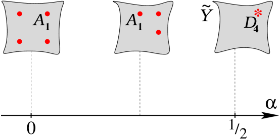
Figure 1. Singularities of $\widetilde{Y}$: $a)$ four simple singularities of type $A_{1}$ when $\alpha=0$, $b)$ one singularity of type $D_{4}$ when $\alpha=\frac{1}{2}$, and $c)$ three $A_{1}$ singularities for all other values $0<\alpha<\frac{1}{2}$.

On the other hand, when $\alpha=0$ (i.e. $a=0$) the mirror geometry (5.21) develops the fourth $A_{1}$ singularity at $(x,y,z)=(-2,-2,-2)$. At this special value of $\alpha$ both $Y$ and $\widetilde{Y}$ take the form of the Cayley cubic (5.6), with possible values of the $B$-field equal to $0$ or $\frac{1}{2}$ in the direction of each exceptional divisor [A]. Which values are realized in our problem can be easily determined via the connection with [Gu], where the same sigma-model played an important role in the gauge theory approach to knot homologies. Thus, in order to understand the basic operations in knot theory (the skein relations) one needs to study the special case of a four-punctured sphere ${\mathbb{C}}{\mathbf{P}}^{1}\setminus\{p_{1},p_{2},p_{3},p_{4}\}$, and the family of cubic surfaces (5.21) is precisely the moduli space of flat $SL(2,\mathbb{C})$ connections on a four-punctured sphere with holonomies $V_{i}$, such that $\operatorname{tr}V_{i}=a$ for all $i=1,\ldots,4$.

Likewise, the original cubic surface (5.3) incidentally is the moduli space of flat $SL(2,\mathbb{C})$ connections on ${\mathbb{C}}{\mathbf{P}}^{1}\setminus\{p_{1},p_{2},p_{3},p_{4}\}$ with holonomy parameters

(5.22) $$\alpha_{1}=\frac{\alpha}{4}-\frac{1}{2}\qquad{\rm and}\qquad\alpha_{2}=\alpha_{3}=\alpha_{4}=\frac{\alpha}{4}\,,$$

where we labeled each holonomy $V_{i}$ by a parameter $\alpha_{i}$ as in (2.17). This fact can be used to determine the value of the $B$-field in the mirror $B$-model of $\widetilde{Y}$. Indeed, the duality maps each holonomy parameter $\alpha_{i}$ to the “quantum” parameter $\eta_{i}$ associated with the $i$-th puncture [GW1],

(5.23) $$\Phi_{{\rm mirror}}~{}:~{}~{}~{}\alpha_{i}\;\rightarrow\;\eta_{i}\,.$$

In the mirror $B$-model with the target space $\widetilde{Y}$, the quantum parameters $\eta_{i}$ describe the flux of the $B$-field through the corresponding $2$-cycles $\widetilde{D}_{i}$. This, together with (5.22), determines the value of the $B$-field:

$$B =: \sum_{i=1}^{4}\eta_{i}\widetilde{D}_{i}$$

$$= \left(\frac{\alpha}{4}-\frac{1}{2}\right)\widetilde{D}_{1}+\frac{\alpha}{4}\widetilde{D}_{2}+\frac{\alpha}{4}\widetilde{D}_{3}+\frac{\alpha}{4}\widetilde{D}_{4}\,.$$

The non-trivial $B$-field has an important effect in the $B$-model of $\widetilde{Y}$. In particular, one should remember that, in the presence of a $B$-field, the Chern character $\operatorname{ch}(\widetilde{\mathcal{B}})$ always appears in a gauge invariant combination $e^{-B}\operatorname{ch}(\widetilde{\mathcal{B}})$ and the charge vector of a brane $\widetilde{\mathcal{B}}$ is given by the modified Mukai vector,

(5.25) $$v({\mathcal{B}})=e^{-B}\operatorname{ch}({\mathcal{B}})\sqrt{{\rm Td}(\widetilde{Y})}\,,$$

instead of (3.47).

As the parameter $\alpha$ gradually varies from $0$ to $\frac{1}{2}$, the geometry of $\widetilde{Y}$ interpolates between the two extreme cases depicted in Figure 1, so that three $A_{1}$ singularities remain unresolved. With our choice of conventions, the corresponding exceptional divisors are $\widetilde{D}_{2}$, $\widetilde{D}_{3}$, and $\widetilde{D}_{4}$. In other words, the 2-cycles $\widetilde{D}_{2}$, $\widetilde{D}_{3}$, and $\widetilde{D}_{4}$ have zero volume with respect to all Kähler forms on $\widetilde{Y}$, whereas ${\rm Vol}(\widetilde{M})$ and ${\rm Vol}(\widetilde{D}_{1})$ vary with $\alpha$ in such a way that their linear combination (5.12) gives the volume of the elliptic fiber,

(5.26) $${\rm Vol}(\widetilde{F})\;=\;2{\rm Vol}(\widetilde{M})+{\rm Vol}(\widetilde{D}_{1})\,,$$

and remains constant (independent of $\alpha$). Indeed, for the cubic surface (5.21) with real values of $a$, only $\widetilde{\omega}_{I}$ has non-zero periods over these 2-cycles, and an easy computation analogous to (5.14) - (5.15) shows that, besides (5.26), the periods obey the following relation,

(5.27) $$\int_{\widetilde{D}_{1}}\widetilde{\omega}_{I}\;=\;2\alpha\int_{\widetilde{F}}\widetilde{\omega}_{I}\,,$$

which will be useful to us below. Note, in particular, that at $\alpha=0$ we have ${\rm Vol}(\widetilde{D}_{1})=0$, whereas at $\alpha=\frac{1}{2}$ the volume of $\widetilde{M}$ vanishes.

Now, let us discuss $(B,B,B)$ branes on $\widetilde{Y}$, in particular, the branes $\widetilde{\mathcal{B}}^{\prime}$ and ${\widetilde{\mathcal{B}}}_{cc}$ which are of major importance in the $B$-model approach to quantization of $M={\mathcal{M}}_{{\rm flat}}(G,C)$. Starting with (3.8), by now we encountered several times one particular $(B,B,B)$ brane, namely a regular zero-brane ${\mathcal{B}}_{p}$, which is dual to a $(B,A,A)$ brane ${\mathcal{B}}_{{F}}$ supported on a generic fiber of $\pi:Y\to{B}$.

In addition, the category of $B$-branes on $\widetilde{Y}$ contains “fractional” zero-branes supported at the orbifold singularities of $\widetilde{Y}$. Specifically, the spectrum of branes at the Kleinian quotient singularity $\mathbb{C}^{2}/\Gamma$ by a finite group $\Gamma\subset SL(2,\mathbb{C})$ is described by ${\mathcal{D}}^{b}_{\Gamma}(\mathbb{C}^{2})$, and fractional branes correspond to the simple objects of this category:

(5.28) $${\mathcal{B}}_{i}\;=\;\varrho_{i}\otimes{\mathcal{O}}_{p}\,.$$

Here, $\varrho_{i}$ are irreducible representations of $\Gamma$ and ${\mathcal{O}}_{p}$ is the skyscraper sheaf supported at the origin of $\mathbb{C}^{2}$. The category of fractional branes is equipped with an action of the tensor category ${\rm Rep}(\Gamma)$. For example, if $\Gamma=\mathbb{Z}_{2}$, as in our model with $0\leq\alpha<\frac{1}{2}$, then at every orbifold point there are two fractional branes ${\mathcal{B}}_{+}$ and ${\mathcal{B}}_{-}$ of charge $v({\mathcal{B}}_{\pm})=(0,\pm 1,\frac{1}{2})$, permuted by the sign representation of $\Gamma=\mathbb{Z}_{2}$ and left invariant by the action of the trivial representation of $\Gamma=\mathbb{Z}_{2}$, cf. [DM, FW]. Note, in this case, each fractional brane carries only a half of the zero-brane charge $v({\mathcal{B}}_{p})=(0,0,1)$,

(5.29) $$v({\mathcal{B}}_{+})+v({\mathcal{B}}_{-})=v({\mathcal{B}}_{p})\,.$$

More generally, in the equivariant category ${\mathcal{D}}^{b}_{\Gamma}(\mathbb{C}^{2})$, the zero-brane ${\mathcal{B}}_{p}$ corresponds to $\varrho_{{\rm reg}}\otimes{\mathcal{O}}_{p}$, where $\varrho_{{\rm reg}}$ is the regular representation of $\Gamma$. The representation $\varrho_{{\rm reg}}$ is reducible and, according to a fundamental theorem of finite group theory, decomposes as $\varrho_{{\rm reg}}=\oplus_{i}d_{i}\varrho_{i}$, where $d_{i}=\dim(\varrho_{i})$ and $\dim(\varrho_{{\rm reg}})=|\Gamma|$. Therefore, in terms of the fractional branes (5.28), we have

(5.30) $${\mathcal{B}}_{p}\;=\;\bigoplus_{\varrho_{i}\in{{\rm Irr}}(\Gamma)}d_{i}{\mathcal{B}}_{i}\,.$$

This provides us with a good supply of $(B,B,B)$ branes localized at the orbifold singularities of $\widetilde{Y}$.

In order to describe $(B,B,B)$ branes on $\widetilde{Y}$ for generic values of $\alpha$, one needs to understand what happens to the fractional branes ${\mathcal{B}}_{i}$ under the minimal resolution of the Kleinian quotient singularity $\mathbb{C}^{2}/\Gamma$. The answer comes from the following equivalence (the derived McKay correspondence)

(5.31) $${\mathcal{D}}^{b}(X)\;\cong\;{\mathcal{D}}^{b}_{\Gamma}(\mathbb{C}^{2})\,,$$

where $X$ denotes the minimal resolution. According to [KV], in the derived category of $X$, the simple objects (5.28) are represented by

(5.32) $$\phantom{\Big{(}x\Big{)}}{\mathcal{B}}_{1} = {\mathcal{O}}_{\sum d_{i}D_{i}}\,,$$

$$\phantom{\Big{(}x\Big{)}}{\mathcal{B}}_{i} = {\mathcal{O}}_{D_{i}}(-1)[1]\,,\qquad i\neq 1\,,$$

where $D_{i}$ are the exceptional divisors. In particular, in the derived category of $X$ it is easy to see that each fractional brane ${\mathcal{B}}_{i}$ is a spherical object, i.e.

(5.33) $$\operatorname{Ext}^{*}_{X}({\mathcal{B}}_{i},{\mathcal{B}}_{i})\;\cong\;H^{*}({\mathbb{C}}{\mathbf{P}}^{1},\mathbb{C})\,.$$

This gives yet another reason to identify the fractional branes on $\widetilde{Y}$ with the duals of Lagrangian $A$-branes supported on irreducible components of the singular fiber (5.9), since each component is a copy of ${\mathbb{C}}{\mathbf{P}}^{1}$, cf. [FW]. (Remember, the first hint came from (5.17), which was then further supported by (5.29) and the fact that $\widetilde{Y}$ has orbifold singularities.)

In order to identify the mirror $(B,B,B)$ branes more carefully, it is convenient to start at $\alpha=\frac{1}{2}$. As we explained earlier, at this special value of $\alpha$ the hypersurface (5.21) develops a singularity of type $D_{4}$ which, luckily, is also a quotient singularity $\mathbb{C}^{2}/\Gamma$ by the binary dihedral group $\Gamma=BD_{8}$, whose action on $\mathbb{C}^{2}$ is generated by the two elements,

(5.34) $$\gamma_{1}\;=\;\begin{pmatrix}\xi&0\\ 0&\xi^{-1}\end{pmatrix}\qquad{\rm and}\qquad\gamma_{2}\;=\;\begin{pmatrix}0&1\\ -1&0\end{pmatrix}\,,$$

with $\xi=\exp(\pi i/2)$. The group $\Gamma=BD_{8}$ has one $2$-dimensional irreducible representation $\varrho_{0}$ and four $1$-dimensional irreducible representations $\varrho_{i}$, $i=1,\ldots,4$ (which altogether can be put into three $2$-dimensional representations, two of which are reducible). Therefore, from (5.30) we find that, at the $D_{4}$ singularity on $\widetilde{Y}$, the zero-brane ${\mathcal{B}}_{p}=\Phi_{{\rm mirror}}({\mathcal{B}}_{{F}})$ is reducible and decomposes as

(5.35) $${\mathcal{B}}_{p}\;=\;2{\mathcal{B}}_{0}\oplus\bigoplus_{i=1}^{4}{\mathcal{B}}_{i}\,.$$

Comparing this to (5.11), one is led to identify ${\mathcal{B}}_{0}$ with $\widetilde{\mathcal{B}}^{\prime}$ and ${\mathcal{B}}_{i}$, $i=1,\ldots,4$ with the branes mirror to the four $(B,A,A)$ branes supported on the exceptional divisors $D_{i}\subset Y$.

Indeed, since all of these $(B,A,A)$ branes are supported on irreducible components of the singular fiber (5.9) over $b=0$, we expect the mirror $(B,B,B)$ branes to be also supported on various components of the singular fiber of $\widetilde{Y}$. In particular, their Chern characters must be linear combinations of the Poincaré duals of the $2$-cycles $\widetilde{M},\widetilde{D}_{1},\ldots,\widetilde{D}_{4}$ and, of course, the class of a point $\operatorname{ch}({\mathcal{B}}_{p})=-p$. Specifically, from (5.32) we find

(5.36) $$\operatorname{ch}(\widetilde{\mathcal{B}}^{\prime})\;=\;\frac{1}{2}\left(-\widetilde{F}+\widetilde{D}_{1}+\widetilde{D}_{2}+\widetilde{D}_{3}+\widetilde{D}_{4}\right)$$

According to (5) and (5.25), as a function of $\alpha$ the $0$-brane charge of the brane $\widetilde{\mathcal{B}}^{\prime}={\mathcal{B}}_{0}$ is equal to $-(\eta_{1}+\eta_{2}+\eta_{3}+\eta_{4})=\frac{1}{2}-\alpha$. This fact plays an important role in the application to the Verlinde formula. Indeed, together with (5.17), it determines the leading contribution to the dimension of ${\mathcal{H}}=\operatorname{Ext}^{*}_{\widetilde{Y}}({\widetilde{\mathcal{B}}}_{cc},\widetilde{\mathcal{B}}^{\prime})$ which, according to (3.4), is given by

(5.37) $$\dim{\mathcal{H}}\;=\;\int_{\widetilde{Y}}\operatorname{ch}({\widetilde{\mathcal{B}}}_{cc})^{*}\wedge\operatorname{ch}(\widetilde{\mathcal{B}}^{\prime})\wedge{\rm Td}(\widetilde{Y})\;=\;k-\lambda+1$$

and matches exactly (5.1) if for ${\widetilde{\mathcal{B}}}_{cc}$ we take the sheaf on $\widetilde{Y}$ that descends from the hyperholomorphic sheaf on $\mathbb{C}^{*}\times\mathbb{C}^{*}$ described in section 3.2.

Indeed, in section 3.2 we discussed a hyperholomorphic sheaf on $\mathbb{C}^{*}\times\mathbb{C}^{*}$ with the Chern character (3.37), which is invariant under the $\mathbb{Z}_{2}$ action. Hence, it can be thought of as a $\mathbb{Z}_{2}$-equivariant coherent sheaf with the trivial $\mathbb{Z}_{2}$-equivariant structure that defines a coherent sheaf ${\widetilde{\mathcal{B}}}_{cc}$ on $\widetilde{Y}$ via the functor

(5.38) $$\Phi~{}:~{}~{}~{}{\mathcal{D}}^{b}_{\mathbb{Z}_{2}}(\mathbb{C}^{*}\times\mathbb{C}^{*})\;\overset{\sim}{\longrightarrow}\;{\mathcal{D}}^{b}(\widetilde{Y})\,,$$

which is an equivalence [BKR] between the bounded derived category of coherent sheaves on $\widetilde{Y}$ and the bounded derived category of $\mathbb{Z}_{2}$-equivariant coherent sheaves on $\mathbb{C}^{*}\times\mathbb{C}^{*}$. To be more specific, the functor (5.38) is obtained by considering the following commutative diagram

(5.39) $$\begin{array}[]{ccc}~{}{\mathcal{Z}}&\;\overset{p}{\longrightarrow}&\mathbb{C}^{*}\times\mathbb{C}^{*}\\ {}^{\kappa}\big{\downarrow}&\;\phantom{\bigg{\downarrow}}&\big{\downarrow}{}^{\kappa^{\prime}}\\ ~{}\widetilde{Y}&\;\overset{p^{\prime}}{\longrightarrow}&(\mathbb{C}^{*}\times\mathbb{C}^{*})/\mathbb{Z}_{2}\end{array}$$

in which $p$ and $p^{\prime}$ are birational, $\kappa$ and $\kappa^{\prime}$ are finite of degree $2$, and $\kappa$ is flat (see [BKR] for further details and examples).

Finally, we note that, with little extra work, one can extend the analysis in the present section to reproduce the Verlinde formula for the four-punctured sphere. In that case, the mirror manifolds $Y$ and $\widetilde{Y}$ are also cubic surfaces, similar to (5.3) and (5.21), which in general depend on four holonomy parameters $\alpha_{1}$, $\alpha_{2}$, $\alpha_{3}$, and $\alpha_{4}$ (that we already found useful in our discussion here). They exhibit a more elaborate structure of singularities (cf. Figure 1) and a rich spectrum of branes that account for the intricate structure of the Verlinde formula (2.18).

Acknowledgments  I would like to thank the organizing committee of the Takagi Lectures for inviting me, and to acknowledge helpful discussions with E. Frenkel, T. Hausel, and E. Witten. I also would like to thank E. Witten for collaboration on the $A$-model approach to quantization reviewed in section 2. This work is supported in part by DOE Grant DE-FG03-92-ER40701 and in part by NSF Grant PHY-0757647. Opinions and conclusions expressed here are those of the author and do not necessarily reflect the views of funding agencies.

References

- [AZ] M. Aldi and E. Zaslow, Coisotropic Branes, Noncommutativity, and the Mirror Correspondence, JHEP 0506 (2005) 019, arXiv:hep-th/0501247.
- [A] P. Aspinwall, Enhanced gauge symmetries and K3 surfaces, Phys. Lett. B357 (1995) 329–334, arXiv:hep-th/9507012.
- [AB] M. Atiyah and R. Bott, The Yang-Mills equations over Riemann surfaces, Phil. Trans. R. Soc. London A 308 (1982) 523–615.
-
[ASS]
M. Atiyah and I. Singer,
The index of elliptic operators I,
Ann. Math. 87 (1968) 484–530;
M. Atiyah and G. Segal, The index of elliptic operators II, Ann. Math. 87 (1968) 531–545;
M. Atiyah and I. Singer The index of elliptic operators III, Ann. Math. 87 (1968) 546–609. - [BFFLS] F. Bayen, M. Flato, C. Fronsdal, A. Lichnerowicz and D. Sternheimer, Deformation Theory and Quantization. I. Deformations of Symplectic Structures, Ann. Physics 111 (1978) 61–110.
- [B] A. Beauville, Vector bundles on curves and generalized theta functions: recent results and open problems, MSRI Publications 28 (1995) 17–33, arXiv:alg-geom/9404001.
- [BNR] A. Beauville, M.S. Narasimhan and S. Ramanan, Spectral curves and the generalised theta divisor, J. Reine Angew. Math. 398 (1989) 169–179.
- [BGV] N. Berline, E. Getzler and M. Vergne, Heat kernels and Dirac operators, Springer-Verlag, Berlin-Heidelber-New York, 1992.
- [BJSV] M. Bershadsky, A. Johansen, V. Sadov and C. Vafa, Topological reduction of 4-d SYM to 2-d sigma models, Nucl. Phys. B 448 (1995) 166, arXiv:hep-th/9501096.
- [BKR] T. Bridgeland, A. King, M. Reid, The McKay correspondence as an equivalence of derived categories, J. Amer. Math. Soc. 14 (2001) 535–554.
- [C] E. Calabi, Métriques Kählériennes et fibrés holomorphes, Ann. Scient. École Norm. Sup., 12 (1979) 269–294.
- [CV] S. Cecotti and C. Vafa, Topological antitopological fusion, Nucl. Phys. B367 (1991) 359–461.
- [CGLP] M. Cvetic, G. W. Gibbons, H. Lu and C. N. Pope, Hyper-Kaehler Calabi metrics, harmonic forms, resolved M2-branes, and correspondence, Nucl. Phys. B617 (2001) 151, arXiv:hep-th/0102185.
- [DM] M. Douglas and G. Moore, D-branes, Quivers, and ALE Instantons, arXiv:hep-th/9603167.
- [D] B. Dubrovin, Integrable systems in topological field theory, Nucl. Phys. B379 (1992) 627–689.
- [FW] E. Frenkel and E. Witten, Geometric Endoscopy and Mirror Symmetry, Communications in Number Theory and Physics, 2 (2008) 113–283 (arXiv:0710.5939).
- [FG] E. Frenkel and S. Gukov, S-duality of branes and geometric Langlands correspondence, to appear.
- [Go] W. Goldman, The modular group action on real -characters of a one-holed torus, Geom. Topol. 7 (2003) 443–486.
- [Gu] S. Gukov, Surface Operators and Knot Homologies, proceedings of the International Congress on Mathematical Physics 2006, Fortsch. Phys. 55 (2007) 473–490, arXiv:0706.2369.
- [GW] S. Gukov and E. Witten, D-branes and Quantization, Adv. Theor. Math. Phys. 13 (2009) 1–73, arXiv:0809.0305.
- [GW1] S. Gukov and E. Witten, Gauge theory, ramification, and the geometric Langlands program, Current Developments in Mathematics 2006 (2008) 35–180.
- [GW2] S. Gukov and E. Witten, Rigid Surface Operators, Adv. Theor. Math. Phys. 14 (2010) 87–177, arXiv:0804.1561.
- [Ha] T. Hausel, Geometry of the moduli space of Higgs bundles, PhD thesis (1998), arXiv:math/0107040.
- [HT] T. Hausel and M. Thaddeus, Mirror symmetry, Langlands duality, and the Hitchin system, Invent. Math. 153 (2003) 197–229, arXiv:math/0205236.
- [Hi] N. Hitchin, The Self-Duality Equations On A Riemann Surface, Proc. London Math. Soc. (3) 33 (1987) 59–126.
- [KV] M. Kapranov and E. Vasserot, Kleinian singularities, derived categories and Hall algebras, Math. Ann. 316 (2000) 565–576, arXiv:math/9812016.
- [KO] A. Kapustin and D. Orlov, Remarks On -Branes, Mirror Symmetry, And The Fukaya Category, J. Geom. Phys. 48 (2003) 84–99, arXiv:hep-th/019098.
- [KW] A. Kapustin and E. Witten, Electric-magnetic Duality And The Geometric Langlands Program, Communications in Number Theory and Physics 1 (2007) 1–236, arXiv:hep-th/0604151.
- [K] M. Kontsevich, Homological algebra of mirror symmetry, Proceedings of ICM, Zurich 1994, vol. I, Birkhäuser (1995) 120–139, alg-geom/9411018.
- [K1] B. Kostant, Quantization and unitary representations. I. Prequantization, Lecture Notes in Math. 170, Springer, Berlin (1970) 87–208.
- [K2] B. Kostant, Line Bundles And The Prequantized Schrodinger Equation, Coll. Group Theoretical Methods in Physics (Marseilles, 1972) 81.
- [M] S. Mukai, Symplectic structure of the moduli of sheaves on an abelian or K3 surface, Invent. Math. 77 (1984) 101; On the moduli space of bundles on K3 surfaces, I, in “Vector Bundles on Algebraic Varieties” Tata Inst. of Fund. Research.
- [S] J.-M. Souriau, Quantification Geometrique, Commun. Math. Phys. 1 (1966) 374.
- [SYZ] A. Strominger, S.-T. Yau and E. Zaslow, Mirror Symmetry Is –duality, Nucl. Phys. B479 (1996) 243–259.
- [T] M. Thaddeus, Topology of the moduli space of stable bundles over a compact Riemann surface, 1990.
- [V] E. Verlinde, Fusion rules and modular transformations in 2d conformal field theory, Nucl. Phys. B300 (1988) 360–376.
- [Ve] M. Verbitsky, Hyperholomorphic sheaves and new examples of hyperkähler manifolds, Mathematical Physics 12, International Press, 1999, arXiv:alg-geom/9712012.
- [Vo] D. A. Vogan, Jr., Singular unitary representations, Lecture Notes in Math. 880, Springer, Berlin (1981) 506–535.
- [W] E. Witten, Quantum Field Theory and the Jones polynomial, Commun. Math. Phys. 121 (1989) 351.
- [W1] E. Witten, On quantum gauge theories in two-dimensions, Commun. Math. Phys. 141 (1991) 153–209.
- [W2] E. Witten, Geometric Langlands And The Equations Of Nahm And Bogomolny, arXiv:0905.4795.
- [W3] E. Witten, A New Look At The Path Integral Of Quantum Mechanics, arXiv:1009.6032.