Origin and Dynamics of the Mutually Inclined Orbits of $\upsilon$ Andromedae c and d

Abstract

We evaluate the orbital evolution and several plausible origins scenarios for the mutually inclined orbits of $\upsilon$ And c and d. These two planets have orbital elements that oscillate with large amplitudes and lie close to the stability boundary. This configuration, and in particular the observed mutual inclination, demands an explanation. The planetary system may be influenced by a nearby low-mass star, $\upsilon$ And B, which could perturb the planetary orbits, but we find it cannot modify two coplanar orbits into the observed mutual inclination of $30^{\circ}$. However, it could incite ejections or collisions between planetary companions that subsequently raise the mutual inclination to $>30^{\circ}$. Our simulated systems with large mutual inclinations tend to be further from the stability boundary than $\upsilon$ And, but we are able to produce similar systems. We conclude that scattering is a plausible mechanism to explain the observed orbits of $\upsilon$ And c and d, but we cannot determine whether the scattering was caused by instabilities among the planets themselves or by perturbations from $\upsilon$ And B. We also develop a procedure to quantitatively compare numerous properties of the observed system to our numerical models. Although we only implement this procedure to $\upsilon$ And, it may be applied to any exoplanetary system.

1 Introduction

The $\upsilon$ Andromedae ($\upsilon$ And) planetary system is the first multiple planetary system discovered beyond our own Solar System around a solar-like star (Butler et al. 1999). Not surprisingly, it has received considerable attention from theoreticians, and in many ways has been a paradigm for gravitational interactions in multiplanet extrasolar planetary systems. At first, research focused on its stability (e.g. Laughlin & Adams 1999; Rivera & Lissauer 2000; Lissauer & Rivera 2001; Laskar 2000; Barnes & Quinn 2001; Goździewski et al. 2001). These investigations showed the system appeared to lie near the edge of instability, although an additional body could survive in between planets b and c (Rivera & Lissauer 2001). Later, attention turned to the apsidal motion (e.g. Stepinski et al. 2000; Chiang & Murray 2002; Malhotra 2002; Ford et al. 2005; Barnes & Greenberg 2006a,c, 2007a), with most investigators considering how the apsidal behavior provides clues to formation mechanisms such as planet-planet scattering or migration via disk torques. The recent direct measurement of the actual masses of planets c and d, and especially their 30^∘ mutual inclination, via astrometry (McArthur et al. 2010) maintains this system’s prominence among known exoplanetary systems. In this investigation, we evaluate planets c and d’s gravitational interactions (ignoring b as its orbit is still only constrained by radial velocity (RV) observations), as presented in McArthur et al. (2010), which place strict constraints on the system’s origin.

Such large mutual inclinations among planets are unknown in our Solar System and hence indicate different processes occurred during or after the planet formation process. We assume $\upsilon$ And c and d formed in coplanar, low eccentricity orbits in a standard planetary formation models (see e.g. Hubickyj 2010; Mayer 2010), but then additional phenomena, occurring late or after the formation process, altered the system’s architecture. We consider two plausible mechanisms: a) If the distant stellar companion $\upsilon$ And B (Lowrance et al. 2002) is on a significantly inclined (relative to the initial orbital plane of the planets) and/or eccentric orbit, it may pump up eccentricities and inclinations through “Kozai” interactions (Kozai 1962; Takeda et al. 2007); or b) If the planets form close together they may interact and scatter into mutually inclined orbits, as shown in previous studies (Weidenschilling & Marzari 2002; Chatterjee et al. 2008; Raymond et al. 2010).

The mutual inclinations are obviously of the most interest, but other features of the system are also important. As $\upsilon$ And represents the first exoplanetary system with full three-dimensional orbits and true masses directly measured (aside from the pulsar system PSR 1257+12 [Wolszczan 1994]), we may exploit this information when evaluating formation models. To that end, we develop a simple metric that quantifies the success of a model at reproducing numerous observed aspects of the $\upsilon$ And planetary system. Although we apply this approach to $\upsilon$ And, it is generalizable to any planetary system.

In this investigation we limit the analysis to just $\upsilon$ And c and d, and to the stable fit presented in McArthur et al. (2010). As described in that paper, the inclination and longitude of ascending node of b are not detectable with the Hubble Space Telescope, so rather than explore the range of architecture permitted by RV data, we focus on the known properties of c and d. Furthermore, we do not consider the range of uncertainties in c and d as the stable fit in McArthur et al. (2010) is surrounded by unstable fits. As we see below, even limiting our scope in this way, we still must perform a large number of simulations over a wide range of parameter space.

We first ($\S$ 2) analyze the current orbital oscillations of $\upsilon$ And c and d with an N-body simulation. We then use the dynamical properties to constrain our two inclination-raising scenarios, which we explore through $>$50,000 N-body simulations. Then in $\S$ 3 we show that $\upsilon$ And B by itself cannot raise the mutual inclinations to $30^{\circ}$. In $\S$ 4 we show that planet-planet scattering is a likely inclination-raising mechanism. However, we find that the most stringent constraint on scattering is the combination of its $30^{\circ}$ mutual inclination and extreme proximity to the stability boundary. In $\S$ 5 we discuss the results and place them in context with previous dynamical and stability studies of exoplanets.

Table 1: Current Configuration of $\upsilon$ And c and d

Planet	$m$ (MJ)	a (AU)	e	$i$ (∘)	$\varpi$ (∘)	$\Omega$ (∘)	$n$ (∘)
c	14.57	0.861	0.24	16.7	290	295	270.5
d	10.19	2.70	0.274	13.5	240.8	115	266.1

2 Orbital Evolution of $\upsilon$ And c and d

In this section we determine the orbital evolution of $\upsilon$ And c and d. As the mass and orbit of planet b are unknown and the four-body interactions between $\upsilon$ And A, b, c and d are extremely complex and depend sensitively on a secular resonance, general relativity and the stellar oblateness (McArthur et al. 2010), we have chosen to leave them out of this analysis, but will address them in a future study.

We examine the secular behavior of the system through an N-body simulation using the Mercury code (Chambers 1999). Here and below we used the “hybrid” integrator in Mercury. Energy was conserved to 1 part in $10^{8}$. For this integration we change the coordinate system from that in the discovery paper, which is based on the viewing geometry, and instead reference our coordinates to the invariable (or fundamental) plane. This plane is perpendicular to the total angular momentum vector of the system (although we ignore planetary spins), i.e. we rotated the coordinate system. The planets’ orbital elements in this coordinate system are listed in Table 1 at epoch JD 2452274.0. The system shown in Table 1 was found to be stable in McArthur et al. , but it was also noted that the system is close to the stability boundary. Therefore we cannot exclude the possibility that other solutions may result in significantly different dynamical behavior. Here and below we assume that such a situation is not the case.

The orbits of planets c and d undergo mutual perturbations which cause periodic variations in orbital elements over thousands of orbits. The long-term changes can be conveniently divided into two parts: the apsidal evolution (changes in eccentricity $e$ and longitude of periastron $\varpi$) and the nodal evolution (changes in inclination $i$, longitude of ascending node $\Omega$, and hence the mutual inclination $\Psi$). The variations, starting with the conditions in Table 1, are shown in Fig. 1. In this figure, we chose a Jacobi coordinate system in order to minimize frequencies due to the reflex motion of the star.

In Fig. 1 the left panels show the apsidal behavior, and the right show the nodal behavior. The lines of apse oscillate about $\Delta\varpi=\pi$, i.e. anti-aligned major axes. This revision once again changes the expected apsidal evolution. Initially Chiang & Murray (2002) and Malhotra (2002) found the major axes oscillated about alignment. Then Ford et al. (2005; see also Barnes & Greenberg 2006a,c) found the system was better described as “near-separatrix,” meaning the apsides lie close to the boundary between libration and circulation. Now we find that the system found by McArthur et al. (2010) librates in an anti-aligned sense! Substantial research has examined the secular behavior of exoplanetary systems, yet the story of $\upsilon$ And shows that predicting the dynamical evolution of a planetary system based on minimum masses and poorly constrained eccentricities is uncertain at best and foolhardy at worst. Even now, without full three-dimensional information about planets b and e (a trend seen in McArthur et al. [2010]) our analysis should only be considered preliminary.

Table 2: Dynamical Properties of $\upsilon$ And c and d

Property	Value
$e^{min}_{c}$	0.069
$e^{min}_{d}$	0.074
$e^{max}_{c}$	0.39
$e^{max}_{d}$	0.365
$\epsilon$	0.17
$i^{min}_{c}$	$16.0^{\circ}$
$i^{min}_{d}$	$11.6^{\circ}$
$i^{max}_{c}$	$20.4^{\circ}$
$i^{max}_{d}$	$16.7^{\circ}$
$\Psi^{min}$	$27.6^{\circ}$
$\Psi^{max}$	$37.1^{\circ}$
$\beta/\beta_{crit}$	1.075

The eccentricities and inclinations undergo large oscillations, as does the mutual inclination. The slow $\sim$15,000 year oscillations are expected from analytical secular theory. The high-frequency oscillation is probably a combination of coupling between eccentricity and inclination and velocity changes that occur during conjunction (note that the impulses at each conjunction can change $e$ by more than 0.01). Note also that the ratio of the orbital period, 5.32, is not very close to the low-order 5:1 and 11:2 resonances, so this high frequency evolution is not due to a mean motion resonance.

The numerical integration also allows a calculation of the proximity to the apsidal separatrix $\epsilon$ (Barnes & Greenberg 2006c). When $\epsilon$ is small ($~{}\hbox to0.0pt{$<$\hss}{\lower 4.30554pt\hbox{$\sim$}}0.01$), two planets are near the boundary between librating and circulating major axes. Although $\upsilon$ And was the first system to be identified as near-separatrix (Ford et al. 2005), we find $\epsilon=0.17$ indicating that the system is actually not close to the separatrix, according to the McArthur et al. (2010) model.

Also of interest is the system’s proximity to dynamical instability, e.g. the ejection of a planet. Previous studies found planets c and d are close to this limit (Rivera & Lissauer 2000; Barnes & Greenberg 2001, 2004; Goździewski et al. 2001). Here we calculate c and d’s proximity to the Hill stability boundary with the quantity $\beta/\beta_{crit}$ (Barnes & Greenberg 2006b,2007b; see also Marchal & Bozis 1982; Gladman 1993; Veras & Armitage 2004). If $\beta/\beta_{crit}>1$ then the pair is stable, if $<1$, it is unstable. We find $\beta/\beta_{crit}=1.075$ and therefore these two planets are very close to the dynamical stability boundary. We caution that constraints based on $\beta/\beta_{crit}$ may be misleading, as Hill stability is strictly only applicable to three-body systems.

In Table 2 we list some statistics of our $10^{6}$ year integration based on 36.5 day output intervals in astrocentric coordinates. Superscripts $min$ and $max$ refer to the minimum and maximum values achieved, respectively. Clearly the actual dynamics of this system depend on the presence and properties of planet b, and, in principle, any additional unconfirmed planets, but without better data on these objects, Table 2 is the best available characterization of the orbital evolution of these two planets. They may also be used to evaluate the origins scenarios described in the following two sections.

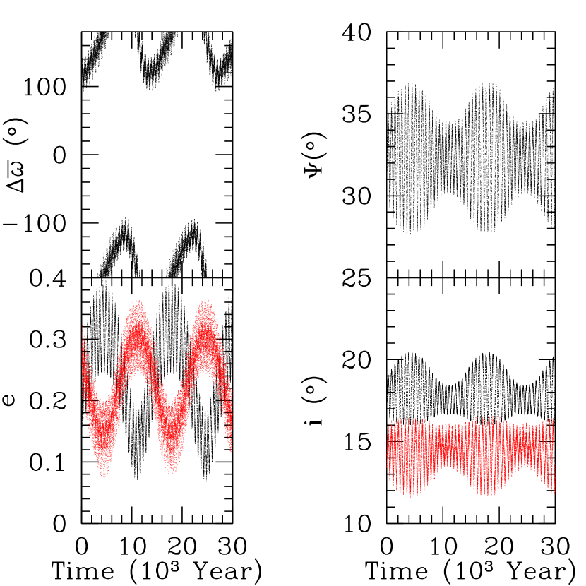
Figure 1: Secular evolution of $\upsilon$ And c (black) and d (red) without planet b. Top left: Evolution of $\Delta\varpi$. Bottom left: Evolution of the eccentricities. Black is planet c, red d. Top right: Evolution of $\Psi$. Bottom right: Evolution of the inclinations. Black is planet c, red d.

3 Perturbations from $\upsilon$ And B

$\upsilon$ And B is a distant M4.5, 0.2 ${\rm\,M_{\odot}}$ companion star to $\upsilon$ And A (Lowrance et al. 2002; McArthur et al. 2010). Its orbit can not be estimated yet, hence we do not know if it is gravitationally bound (Patience et al. [2002]; Raghavan et al. [2006]). Estimates for their separation range from 702 AU (Raghavan et al. 2006) to as much as 30,000 AU (McArthur et al. 2010). If planet c and d formed on circular, coplanar orbits, then could $\upsilon$ And B have pumped up the mutual inclinations of c and d?

Given the uncertainty in B’s orbit, we consider a broad parameter space sweep: 13,200 simulations that cover the range $500\leq a_{B}\leq 2000$ AU, $0.5\leq e_{B}\leq 0.85$ and $30^{\circ}\leq i_{B}\leq 80^{\circ}$. Here $i_{B}$ is referenced to the initial orbital plane of the planets, not the invariable plane of the four-body system. The angular elements were varied uniformly from 0 to 2$\pi$. Note that this range was chosen to increase the perturbative effects of B and does not reflect any expectation of its actual orbit. Each simulation was run for $5\times 10^{6}$ years, which corresponds to $\sim 250$ orbits of B. While not a long time, we find that B may destabilize the planetary system, which could lead to large mutual inclinations of planet c and d (see $\S$ 4).

For the vast majority of these cases, the orbits of c and d remain coplanar, with $\Psi<1^{\circ}$. However, 3 simulations ejected planet d; 192 led to planets with $\Psi^{max}>1^{\circ}$; 26 with $\Psi^{max}>10^{\circ}$; and 1 case out of the 13,200 reached $\Psi^{max}=34^{\circ}$. The 192 non-planar cases were spread throughout parameter space, with no significant clustering.

To explore effects on longer timescales, we integrated 20 cases to 1 Gyr. Four of the previous simulations that had led to significant mutual inclinations (including that which led to $\Psi^{max}=34^{\circ}$) were tested, in order to examine stability. The other 16 were chosen from among those in which $\Psi^{max}$ stayed $<1^{\circ}$ over 250 orbits of B, in order to determine if mutual inclinations could develop over longer timescales. We find that most of these simulations, in fact, ejected a planet. Therefore the orbit of $\upsilon$ And B appears able to destabilize a circular, coplanar system.

Next we relax the requirement that the planets began on coplanar orbits and ran simulations with initial mutual inclinations $\Psi_{0}=3^{\circ}$, $10^{\circ}$, and $30^{\circ}$, and with $a_{B}=700$, $e_{B}=0$, $i_{B}=30^{\circ}$. The two planets began with their current best fit semi-major axes and masses, but on circular orbits, and one inclination was set to $3^{\circ}$, $10^{\circ}$ or $30^{\circ}$ with the masses held constant. These systems were integrated for 1 Gyr. In each of these cases, shown in Fig. 2, the initial value of $\Psi$ is maintained for the duration of the simulation. The widths of the libration increase with $\Psi_{0}$ because the interactions among the planets are driving a secular oscillation. It therefore seems that even if the planets began with a nonzero relative inclination, $\upsilon$ And B is unable to pump it to the range shown in Fig. 1. These simulations also demonstrate that plausible orbits of $\upsilon$ And B will not destabilize the observed system.

These simulations indicate that it is unlikely that $\upsilon$ And B could have twisted the orbits into the mutually inclined system we see today. However, it could have destabilized the system, which we will see in the next section is a process which can lift coplanar orbits to $\Psi~{}\hbox to0.0pt{$>$\hss}{\lower 4.30554pt\hbox{$\sim$}}30^{\circ}$.

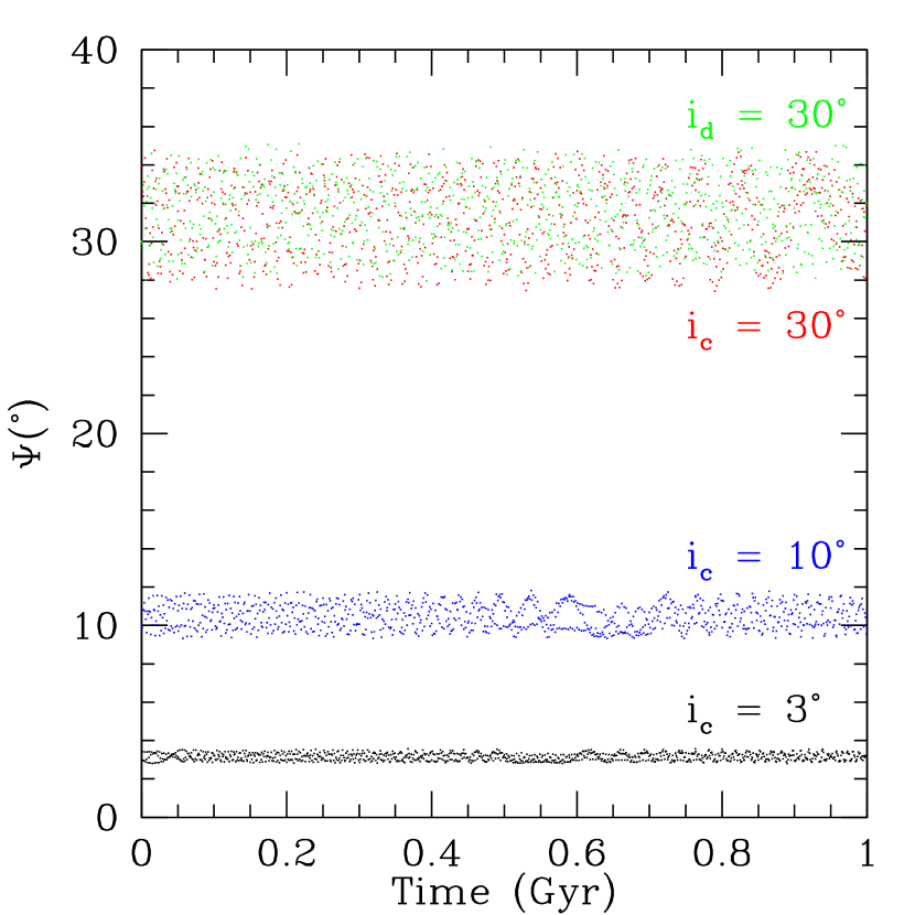
Figure 2: Variation of $\Psi$ for four hypothetical systems with $\upsilon$ And B included (see text for more details). The black points are systems in which initially $i_{c}=3^{\circ}$, blue $i_{c}=10^{\circ}$, red $i_{c}=30^{\circ}$, and green $i_{d}=30^{\circ}$.

4 Planet-Planet Scattering

Our second hypothesis considers the possibility that the planetary system formed in an unstable configuration independent of B, and that encounters between planets ultimately ejected an original companion leaving a system with high mutual inclinations. Such impulsive interactions could drive inclinations to large values, perhaps as large as $60^{\circ}$ (Marzari & Weidenschilling 2002; Chatterjee et al. 2008; Raymond et al. 2010). We considered 41,000 different initial configuration of the system, e.g. one or two additional planets with masses in the range 1 – 15 M${}_{\textrm{Jup}}$. At the end of this section we summarize the results of all these simulations, but initially we focus on one subset.

We completed 5,000 simulations that began with three 10 – 15 M${}_{\textrm{Jup}}$ mass objects (uniformly distributed in mass) separated by 4–5 mutual Hill radii (Chambers et al. 1996), with $e<0.05$, $i<1^{\circ}$ and $0.75<a<4$ AU. We integrated these cases for $10^{6}$ years with Mercury’s hybrid integrator, conserving energy to 1 part in $10^{4}$. About 1% of cases failed to conserve energy at this level and were thrown out. These ranges are somewhat arbitrary but follow the recent study by Raymond et al. (2010), which considered smaller mass planets at larger distances. They found that a system consisting of three 3 M${}_{\textrm{Jup}}$ planets could, after removal of one planet and settling into a stable configuration, end up with $\Psi>30^{\circ}$ about 15% of the time (down from 30% for three Neptune-mass planets). However, they also found that only 5% of systems of three 3 M${}_{\textrm{Jup}}$ planets settled into a configuration with $\beta/\beta_{crit}<1.1$. Therefore we expect that these two parameters will be the hardest to reproduce via scattering. As we see below, this expectation is borne out by our modeling.

In our study, a successful model conserved energy adequately (1 part in $10^{4}$), removed the extra planet, and the remaining planets all had orbits with $a<10$ AU. 2072 trials met these requirements (1416 collisions and 656 ejections). We ran each of these final two-planet configurations for an additional $10^{5}$ years (again validating the simulation via energy conservation) to assess secular behavior for comparison with the system presented in Table 2.

In Fig. 3 we show the outcome of one such trial in which a hypothetical planet was ejected. The format of this figure is the same as Fig. 1. The behavior is qualitatively similar as in Fig. 1, including anti-aligned libration of the apses, the magnitudes of the eccentricities and the inclinations, and the short period oscillation superposed on the longer oscillation. The mutual inclination for this case is even larger than the observed system. This system’s $\beta/\beta_{crit}$ is 1.06, slightly lower than the observed system. This simulation, which is one of the closest matches to the observed system, shows that the ejection of a single additional planet could have produced the $\upsilon$ And system.

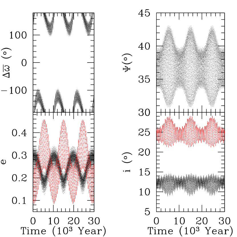
Figure 3: Secular evolution of a simulated system after the ejection of an exterior planet.Top left: Evolution of $\Delta\varpi$. Bottom left: Evolution of the eccentricities. Black is planet c, red d. Top right: Evolution of $\Psi$. Bottom right: Evolution of the inclinations.

Figure 3 is but one outcome. We next explore the statistics of this suite of simulations and consider the other orbital elements and dynamical properties. We divide the outcomes into two cases: Ejections and Collisions. These two phenomena could produce significantly different outcomes. For example, collisions tend to occur near periastron of one planet and apoastron of the other, and we might expect the merged body to have a lower eccentricity than either of the progenitors. We show the cumulative distributions of the properties listed in Table 2 in Fig. 4. Comparing the values of orbital elements at a given time is not ideal, but as it has been done many times (see e.g. Ford et al. 2001; Ford & Rasio 2008; Juric & Tremaine 2008; Chatterjee et al. 2008; Raymond et al. 2010), we do so here as well. In Figs. 4a–c, we show the values of $e$, $i$, and $\Psi$ at the end of the initial $10^{5}$ year integration.

In panels d–h we show the ranges of $i^{min}$, $i^{max}$, $\Psi^{min}$ and $\Psi^{max}$. We find that 8.9% of successful models produced a system with $\Psi^{max}>30^{\circ}$, consistent with Raymond et al. (2010). Note that ejections produce $\Psi^{max}>30^{\circ}$ about 20% of the time.

In Fig. 4i we show the $\epsilon$ distribution, which is bimodal with one peak near 0.1 and another near $10^{-3}$. The observed value of 0.17 is not an unusual value, and we find that systems with this $\epsilon$ value can have appropriate values of $e^{min}$ and $e^{max}$. We note that the significant fraction of systems near the apsidal separatrix contradicts the results of Barnes & Greenberg (2007a), which found that scattering only produced $\epsilon<0.01$ a few percent of the time. The most likely explanation for this difference is that Barnes & Greenberg considered coplanar orbits and forbade collisions, whereas here we explore non-planar motion. Our results also indicate that near-separatrix motion is likely a result of collisions, rather than ejections, and $\epsilon<10^{-4}$ (which is unlikely to be measured any time soon) only result from collisions.

Figure 4j shows the distribution of $\beta/\beta_{crit}$ after scattering. Here the difference between collisions and ejections is starkest: Ejections have a much broader distribution than collisions. Barnes et al. (2008) noted that systems are “packed” (no additional planets can lie in between two planets) when $\beta/\beta_{crit}~{}\hbox to0.0pt{$<$\hss}{\lower 4.30554pt\hbox{$\sim$}}2$, which is near the peak of the ejection distribution. Our results consistent with Raymond et al. (2009).

In this model the mutual inclinations and proximity to instability are the strongest constraints on the system’s origins, but we may quantify scattering’s ability to reproduce all the observed features of the system. Most previous studies of scattering have focused on reproducing eccentricity distributions, but all available information should be used. With this goal in mind, we lay out here a simple method to quantify any model’s ability to reproduce observations. For each simulated system, we calculate its “parameter space distance” $\rho$ from the best fit. We define this quantity as

$$\rho=\sqrt{\sum{\Big{(}\frac{\eta-\eta_{j}}{\eta}\Big{)}^{2}}},$$ (1)

where $\eta$ represents $e^{min}_{j}...\beta/\beta_{crit}$ and $j$ = c,d (see Table 2). This statistic has several limitations: It ignores correlations between parameters; is dependent on the coordinate system; ignores uncertainties in the observations (as discussed above), and possibly overweights some parameters by including combinations of variables that are not independent. Although crude, $\rho$ does provide a quantitative estimate of how close a modeled system is to the observed system. Smaller values of $\rho$ signal a system that is a closer match to the actual system.

In Fig. 4k we plot the distributions of $\rho$. These distributions resemble the $\beta/\beta_{crit}$ distributions (panel j), suggesting it is the most important constraint on the system. In Table 3 we show some statistics of our runs, where “min” is the minimum value of the set, “avg” is the mean, $\sigma$ is the standard deviation, and “max” is the maximum value.

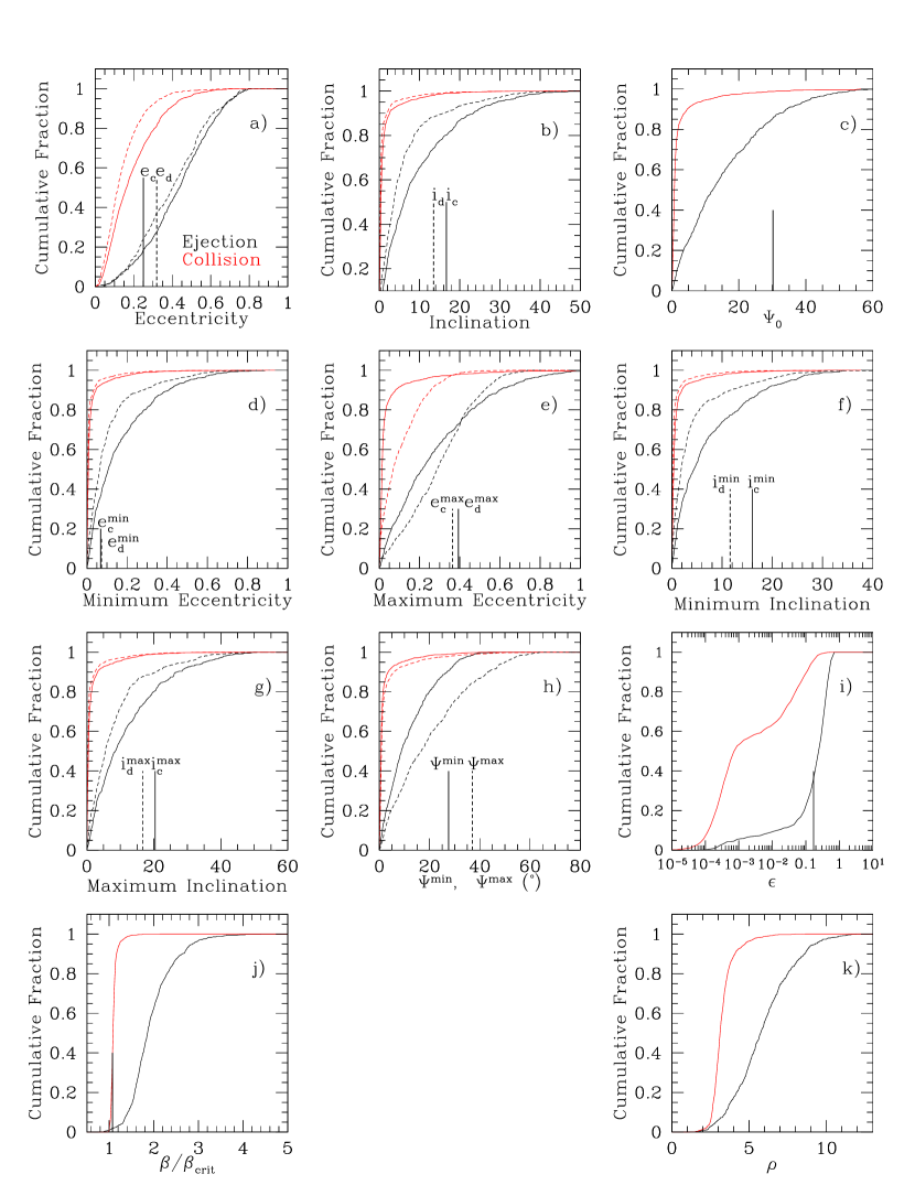
Figure 4: Cumulative distributions of properties (out of 626 ejections, 1416 collisions) after scattering of one planet. Black curves refer to cases in which one planet was ejected, red to a collision between two planets. Thick vertical lines correspond to the value for the best fit system. If the parameter is measurable for both planets, solid lines indicate planet c, dashed d.

For most of the parameters we consider, ejections and collisions do a reasonable job of producing the observed values. However, this representation does not show any cross-correlation, i.e. does a system with high $\Psi$ also have low $\beta/\beta_{crit}$? We explore this relationship in Fig. 5. We see that post-collision systems (blue points) cluster heavily at low $\beta/\beta_{crit}$ and $\Psi^{max}$, but post-ejection systems (red points) have a much broader range. Nonetheless, the two outcomes seem equally likely to reproduce the system, represented by the “+” (recall that there are three times as many blue points as red). However, from our models the actual probability that instabilities can reproduce the $\upsilon$ And system is less than 1%.

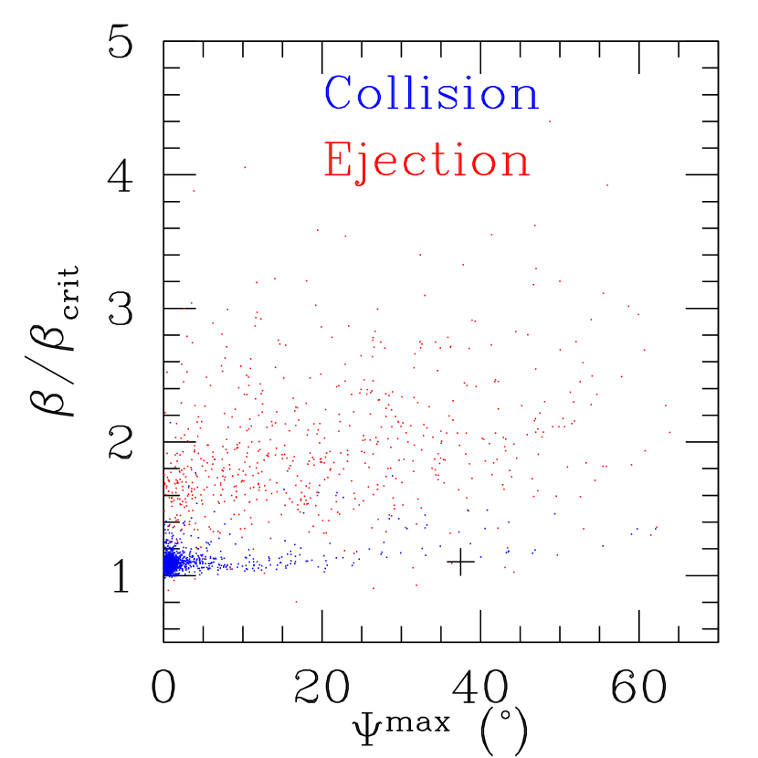
Figure 5: Relationship between proximity to instability ($\beta/\beta_{crit}$) and maximum mutual inclination ($\Psi^{max}$). Systems which experienced a collision are color-coded blue, ejections red. The best fit to the $\upsilon$ And system is shown by the + sign.

From our analysis of these 2072 systems, we see that it is possible for planetary ejections and collisions to reproduce the observed $\upsilon$ And system, albeit with low probability. This suite of simulations is obviously limited in scope, so we performed 36,000 more simulations relaxing constraints on planetary mass (allowing uniform values between 1 and 15 M${}_{\textrm{Jup}}$), separation (uniform distribution between 2 and 5 mutual Hill radii), and number of planets (3 or 4). These other simulations began with two planets with approximately the same semi-major axes as observed, and placed planets interior and/or exterior to these two planets. These simulations show that the equal-mass case we considered here is the best method to achieve large $\Psi$, as expected from Raymond et al. (2010). For additional planets with masses less than 5 M${}_{\textrm{Jup}}$, $\Psi$ values greater than $30^{\circ}$ are very unlikely, but $\beta/\beta_{crit}\sim 1$ is more likely. The removal of two planets does not make much difference in the resulting system. We conclude that the removal of 1 or more planets with mass(es) larger the 5 M${}_{\textrm{Jup}}$ is a viable process to produce the observed configuration of $\upsilon$ And c and d.

Table 3: Distribution of Properties After Collision/Ejection Property Ejection Collision min avg $\sigma$ max min avg $\sigma$ max $e^{min}_{c}$ $3.5\times 10^{-5}$ 0.29 0.17 0.74 $6\times 10^{-6}$ 0.1 0.1 0.64 $e^{min}_{d}$ $7.6\times 10^{-5}$ 0.28 0.19 0.75 $8\times 10^{-6}$ 0.03 0.07 0.51 $e^{max}_{c}$ 0.097 0.53 0.16 0.83 0.024 0.26 0.15 0.79 $e^{max}_{d}$ 0.064 0.28 0.16 0.88 0.05 0.25 0.12 0.77 $\epsilon$ $10^{-4}$ 0.26 0.22 1.36 $3.7\times 10^{-5}$ 0.066 0.12 1.1 $i^{min}_{c}$ (^∘) 0.02 7.2 7.50 34.4 0.013 1.2 2.7 30.4 $i^{min}_{d}$ (^∘) 0.002 4.1 5.9 43.7 0.005 0.77 2.1 30.4 $i^{max}_{c}$ (^∘) 0.08 11.9 10.8 50.8 0.014 1.7 3.8 43.0 $i^{max}_{d}$ (^∘) 0.03 8.3 8.7 48.7 0.007 1.26 3.4 49.7 $\Psi^{min}$ (^∘) 0.06 11.7 9.7 46.8 0.036 2.0 4.5 39.8 $\Psi^{max}$ (^∘) 0.1 19.8 15.5 63.9 0.032 2.9 6.7 62.1 $\beta/\beta_{crit}$ 0.8 1.95 0.49 4.4 0.98 1.11 0.08 2.14 $\rho$ 1.17 5.9 1.9 11.9 1.08 3.3 0.75 8.6

5 Conclusions

We have shown that the orbital behavior of the model for Ups And c and d proposed by McArthur et al. (2010) is quite different from that of orbital models identified by previous studies that had no knowledge of the inclination or actual mass of the planets. The major axes librate in an anti-aligned configuration, and their mutual inclination is substantial and oscillates with an amplitude of about $10^{\circ}$.

We find that the companion star $\upsilon$ And B by itself cannot pump the mutual inclination up to large values, even if the planets began with a significant relative inclination. However, it may have sculpted the planetary system by inciting an instability that ultimately led to ejections of formerly bound planets. The timescale to develop these instabilities is long. The configurations of B that could have such effects are sparsely distributed over parameter space, and the orbits of previously bound planets cannot be specified. These factors make the role of $\upsilon$ And B complicated, but suggest an in-depth analysis of its role merits further research.

Even without B, planet-planet scattering may have driven the system to the observed state. That process can easily reproduce the apsidal motion, but pumping the mutual inclination up to the observed values is difficult and probably requires the removal of a planet with mass $>5$ M${}_{\textrm{Jup}}$. Removing two planets does not increase this probability significantly.

The other important constraint on the scattering hypothesis is the system’s close proximity to the stability boundary, $\beta/\beta_{crit}$. Collisions may leave a system near that boundary, whereas ejections tend to spread out the planets. Furthermore, we find that collisions tend to produce systems with low $\beta/\beta_{crit}$ and low $\Psi$, while ejections produce a broad range of $\Psi$, but large values of $\beta/\beta_{crit}$. Nonetheless, Fig. 3 demonstrates that scattering can produce systems similar to $\upsilon$ And.

Although scattering is a reasonable process to produce the observed architecture, we cannot determine the triggering mechanism. Did scattering occur because $\upsilon$ And B destabilized the planetary system? Or did the planet formation process itself, independent of B, ultimately lead to instabilities? The presence of $\upsilon$ And B makes distinguishing these possibilities very difficult. A larger census of mutual inclinations and stellar companions can resolve this open issue.

Alternatively, our decisions about the system at the onset of scattering could be mistaken. We assumed the planets formed inside the original protoplanetary disk with inclinations $<1^{\circ}$. It may be that larger initial inclinations are possible prior to scattering, in which case the planets could be pumped to larger mutual inclinations (Chatterjee et al. 2008). However, it remains to be seen if such configurations are possible prior to scattering. Future studies should explore the inclinations of giant planets during formation.

We have also ignored the effects of planet b, stellar companion B, and a possible fourth planetary companion (McArthur et al. 2010) in our analysis. These bodies could significantly change the secular behavior, and/or the observed fundamental plane. Furthermore, planet b is tidally interacting with its host star, which could alter the long-term secular behavior (Wu & Goldreich 2002). Hence future revisions to this system, and the inclusion of tidal effects, could significantly alter the interpretations described above, possibly making scattering more likely to produce the observed system. We are currently exploring the wide range of $i$’s and $\Omega$’s of b and the subsequent orbital evolution of the entire system.

Figure 4i shows that scattering tends to produce two types of apsidal behavior: near-separatrix ($\epsilon<10^{-3}$) and motion far from the separatrix ($\epsilon>0.01$) with a desert in between. Adding a second scatterer to the mix does not erase this bimodality. This result contrasts with the case with no inclinations (Barnes & Greenberg 2007a), in which near-separatrix motion ($\epsilon<0.01$) is not a common outcome of scattering. Fig. 4i shows that, in fact, both outcomes are likely, at least in systems similar to $\upsilon$ And. Although there are hints of this structure in the observed exoplanet population (Barnes & Greenberg 2006c), those results are based on radial velocity data. We now know that minimum masses are not necessarily a good indicator of apsidal motion.

For $\upsilon$ And, the large mutual inclination and proximity to instability are strong constraints on the origin of its planetary system. However, for other systems, this may not be the case. We outlined in $\S$ 4 a method in which all aspects of a planetary system can be combined to quantify the validity of a formation model. When the mass and three dimensional orbits of a planetary system are known, the properties presented in Table 1 can be combined into a single parameter $\rho$ which provides a statistic for quantitatively comparing models. In our analysis we ignored the observational errors, which is regrettable, but necessary due to the system’s extreme proximity to dynamical instability (McArthur et al. 2010). We encourage future studies that strive to reproduce the system of McArthur et al. to find $\rho$ values less that those listed in Table 3, as lower values imply a closer match to the system, assuming that other stable solutions show similar behavior to the one we describe here. Furthermore, investigations into exoplanet formation could compare distributions of observed and simulated properties as a quantitative method for model validation.

The revisions of McArthur et al. (2010) reveal the importance of the mass-inclination degeneracy in dynamical studies of exoplanets. Clearly in some cases masses can be much larger than the minimum value measured by radial velocity, which in turn changes secular frequencies and eccentricity amplitudes. However, large changes in mass due to the mass-inclination degeneracy should be rare, hence, trends using minimum masses may still be valid. Nonetheless, we urge caution when exploring trends among dynamical properties (e.g. Zhou & Sun 2003; Barnes & Greenberg 2006c), as they may be misleading.

Even if $30^{\circ}$ mutual inclinations turn out to be rare, systems with $\Psi\sim 10^{\circ}$ probably are not (Fig. 4; Chatterjee et al. 2008; Raymond et al. 2010). If these systems host planets with habitable climates, they may be very different worlds than Earth. Planetary inclinations can drive obliquity variations in terrestrial planets (Atobe et al. 2004, Armstrong et al. 2004; Atobe & Ida 2007), unless they have a large moon (Laskar 1997). Therefore future analyses of potentially habitable worlds should pay particular attention to the mutual inclinations, and climate modeling should explore the range of possibilities permitted by large mutual inclinations. Terrestrial planets will likely be discovered in their star’s habitable zone in the coming years. The orbital configuration and evolution of $\upsilon$ And warns us that habitability assessment hinge on the orbital architecture of the entire planetary system.

RB acknowledges support from the NASA Astrobiology Institute’s Virtual Planetary Laboratory lead team, supported by cooperative agreement No. NNH05ZDA001C. RG acknowledges support from NASA’s Planetary Geology and Geophysics program, grant No. NNG05GH65G. BEM and GFB acknowledge support from NASA through grants GO-09971, GO-10103, and GO-11210 from the Space Telescope Science Institute, which is operated by the Association of Universities for Research in Astronomy (AURA), Inc., under NASA contract NAS5-26555. We also thank Sean Raymond for helpful discussions.

References

- (1) Armstrong, J.C., Leovy, C.B., & Quinn, T.R. 2004, Icarus, 171, 255
- (2) Atobe, K., Ida, S. & Ito, T. 2004, Icarus, 168, 223
- (3) Atobe, K., Ida, S. 2007, Icarus, 188, 1
- (4) Barnes, R., Goździewski, K., & Raymond, S.N. 2008, ApJ, 680, L57
- (5) Barnes, R. & Greenberg, R. 2006a, ApJ, 652, L53
- (6) ————. 2006b, ApJ, 638, 478
- (7) ————. 2006c, ApJ, 647, L163
- (8) ————. 2007a, ApJ, 665, L67
- (9) ————. 2007b, ApJ, 659, L53
- (10) Barnes, R. & Quinn, T.R. 2001, ApJ, 554, 884
- (11) ————. 2004, ApJ, 611, 494
- (12) Barnes, R. & Raymond, S.N. 2004 ApJ, 617, 569
- (13) Butler, R.P. et al. 1999, ApJ, 526, 916
- (14) Chambers, J., 1999, MNRAS, 304, 793
- (15) Chatterjee, S. et al. 2008, ApJ, 686, 580
- (16) Chiang, E. I., Tabachnik, S., & Tremaine, S. 2001, AJ, 122, 1607
- (17) Ford, E.B., Lystad, V., & Rasio, F.A. 2005, Nature, 434, 873
- (18) Ford, E.B. & Rasio, F.A. 2008, ApJ, 686, 621
- (19) Gladman, B. 1993, Icarus, 106, 247
- (20) Goździewski, K. et al. 2001, A&A, 378, 569
- (21) Hubickyj, O. 2010, in Formation and Evolution of Exoplanets, Rory Barnes (ed), Wiley-VCH, Berlin.
- (22) Jurić, M. & Tremaine, S. 2008, ApJ, 686, 603
- (23) Kozai, Y. 1962, AJ, 67, 591
- (24) Laskar, J. 2000, PhRvL, 84, 3240
- (25) Laskar, J., Joutel, F., & Robutel, P. 1993, Nature, 615
- (26) Laughlin, G. & Adams, F.C. 1999, ApJ, 526, 881
- (27) Lissauer, J.J. & Rivera, E.J. 2001, ApJ, 554, 1141
- (28) Lowrance, P.J., Kirkpatrick, J.D., & Beichman, C.A. 2002, ApJ, 572, L79
- (29) Malhotra, R. 2002, ApJ, 575, L33
- (30) Marchal, C. & Bozis, G. 1982, CeMDA, 26, 311
- (31) Marzari, F. & Weidenschilling, S. 2002, Icarus, 156, 570
- (32) Mayer, L. 2010 in Formation and Evolution of Exoplanets, Rory Barnes (ed), Wiley-VCH, Berlin.
- (33) McArthur, B. et al. 2010, ApJ, 715, 1203
- (34) Murray, C.D. & Dermott, S.F. 1999, Solar System Dynamics, Cambridge UP, Cambridge
- (35) Patience, J. et al. 2002, ApJ, 581, 654
- (36) Raymond, S.N. et al. 2009, ApJ, 696, L98
- (37) ————. 2010, ApJ, 711, 772
- (38) Rivera, E.J. & Lissauer, J.J. 2000, ApJ, 530, 454
- (39) Stepinski, T.F., Malhotra, R. & Black, D.C. 2000, 545, 1044
- (40) Takeda, G. & Rasio, F.A. 2005, ApJ, 627, 1001
- (41) Veras, D., & Armitage, P. 2004, Icarus, 172, 349
- (42) Wolf, S. & Klahr, H, 2002, ApJ, 578, L79
- (43) Wolszczan, A. 1994, Science, 264, 538
- (44) Wu, Y., & Goldreich, P. 2002, ApJ, 564, 1024
- (45) Zhou, J.-L., & Sun, Y.-S. 2003, ApJ, 598, 1290
- (46)