Relaxation of spins due to a magnetic field gradient, revisited; Identity of the Redfield and Torrey theories

Abstract

There is an extensive literature on magnetic gradient induced spin relaxation. Cates, Schaefer and Happer (CSH, CSH ), in a seminal paper, have solved the problem in the regime where diffusion theory (the Torrey equation Tor ) is applicable using an expansion of the density matrix in diffusion equation eigenfunctions and angular momentum tensors. McGregor McG has solved the problem in the same regime using a slightly more general formulation using Redfield theory formulated in terms of the auto-correlation function of the fluctuating field seen by the spins and calculating the correlation functions using the diffusion theory Green’s function. The results of both calculations were shown to agree for a special case, McG . In the present work we show that the eigenfunction expansion of the Torrey equation yields the expansion of the Green’s function for the diffusion equation thus showing the identity of this approach with that of Redfield theory. The general solution can also be obtained directly from the Torrey equation for the density matrix. Thus the physical content of the Redfield and Torrey approaches are identical. We then introduce a more general expression for the position autocorrelation function of particles moving in a closed cell, extending the range of applicability of the theory.

year number number identifier Date text]date

LABEL:FirstPage101 LABEL:LastPage#1102

I Introduction

The problem of relaxation in nuclear magnetic resonance due to field gradients has been discussed by many authors but continues to be a topic of current research. Recently attention has been focussed on this subject in connection with searches for new P,T violating forces mediated by the hitherto unobserved Axion Petu , poko .

We give a short, very incomplete, summary of how the field developed until now. In 1950 Hahn Hah used his just invented spin echo technique to study the effect of translational diffusion on relaxation in nmr. Torrey, in 1953 Tor2 gave a derivation of the effect of translational diffusion that had been alluded to by Hahn. In 1954 Carr and Purcell CarrP presented a more elaborate method for measuring diffusion constants using relaxation due to translational diffusion in an inhomogeneous field with known gradient. Then in 1956 Torrey Tor introduced a specific partial differential equation (Torrey equation) describing the effects of diffusion on relaxation. He showed that under conditions when diffusion theory was valid the physics was described by adding a diffusion term to the usual Bloch equations. These treatments of diffusion did not take into account the effect of the boundaries of the measurement cell. Ten years later (1966) Baldwin Robertson ROB gave an approximate solution of the Torrey equation in a relatively small region, defined by 2 parallel planes, where the influence of the boundaries was important. Using the method of phase accumulation and assuming the phase distribution to be Gaussian, Neuman, in 1973 Neum gave an approximate solution for planar, cylindrical and spherical geometries and showed this was in agreement with Robertson’s results.

In 1987, Cates, Schaefer and Happer (CSH) CSH calculated the relaxation for parameters where the diffusion theory is appropriate using second order perturbation theory and an expansion in eigenfunctions of the Torrey equation applied to the density matrix. At high densities the perturbation theory breaks down and at low densities ($\lambda\gtrsim R)$ the diffusion theory is invalid. (The present work shows how to go beyond this latter limit.) The authors start with the equation of motion for the density matrix in the presence of diffusion, (Torrey equation) Tor

$$\frac{\partial\rho}{\partial t}=\frac{1}{i\hbar}\left[H,\rho\right]+D\nabla^{2}\rho$$ (1)

They consider the deviations of the magnetic field from the volume averaged field as a perturbation and the volume averaged field (taken along $z$) as the unperturbed system. Then, expanding $\rho$ in the ’eigenpolarizations’ of the unperturbed problem and carrying out a perturbation expansion in the field variation, taken to be varying linearly with position, they obtain a solution valid to second order in the perturbation.

McGregor McG has given a slightly more general treatment based on Redfield’s relaxation matrix theory Red , as presented by Slichter Sli . The starting point of this treatment is the equation of motion for the density matrix expanded to second order in a perturbation (Sli , equation 5.313)

$$\frac{\partial\rho^{\ast}}{\partial t}=\frac{1}{i\hbar}\left[H_{1}^{\ast}\left(t\right),\rho^{\ast}\left(0\right)\right]+\left(\frac{i}{\hbar}\right)^{2}\int_{0}^{t}\left[\left[\rho^{\ast}\left(0\right),H_{1}^{\ast}\left(t^{\prime}\right)\right],H_{1}^{\ast}\left(t\right)\right]dt^{\prime}$$ (2)

where $H_{1}^{\ast}$ represents the deviation of the field from its volume averaged value and starred quantities are expressed in the interaction representation with the volume average field considered as the unperturbed system.

The results show that the relaxation depends on the auto-correlation function of the fluctuating field (frequency spectrum of the field fluctautions) as seen by the spins as they move through the measurement cell and the correlation function is determined by the diffusion theory Green’s function for the case when diffusion theory is valid.

For high densities, when the boundary conditions do not play a role, the exact solution obtained by Torrey Tor is valid.

Following this work in 1991, Stoller, Happer and Dyson STHappDyson  have shown how to use the exact eigenfunctions of the Torrey equation (Airy functions) to get exact solutions in one dimension. de Swiet and Sen deSwSen have used this and other approaches to study a wider range of geometries. Hayden et al (2004) give a nice discussion of the Gaussian phase distribution work along with experimental confirmation in a cylindrical geometry MHayd .

McGregor McG has shown that the results of his Redfield theory treatment are equivalent to those obtained from the Torrey equation CSH for the special case of the high pressure limit in a spherical cell. Nevertheless it is illuminating to note that the expansion in the diffusion equation eigenfunctions obtained by CSH CSH is in fact the usual eigenfunction expansion of the Green’s function and hence the results based on the Torrey equation CSH and those of the Redfield theory McG are identical for all cases considered by CSH. We show this in the next section, with details confined to an appendix. Thus the physical content of the two approaches are identical in spite of their rather different starting points.

We then show how these results can be applied beyond the diffusion theory limits by giving an analytic expression for the trajectory correlation functions valid for a range of pressures wider than that for which diffusion theory is applicable.

II Equivalence of the Torrey equation and Redfield theory results when diffusion theory is valid.

In the appendix we review the calculation of CSH applied to spin 1/2 and using a slightly altered notation. We expand the density matrix in the spin 1/2 operators, $\sigma_{0,\pm 1}.$

The result for $T_{1}$, equation (79), compare equation (50), CSH:

$$\frac{1}{T_{1}}=\frac{4}{V}\operatorname{Re}\int\int\left[\Omega_{1}\left(\overrightarrow{r^{\prime}}\right)\right]_{-}\left[\Omega_{1}\left(\overrightarrow{r}\right)\right]_{+}\sum_{\beta^{\prime}}\ \left(\frac{\phi_{\beta^{\prime}}\left(\overrightarrow{r}^{\prime}\right)\phi_{\beta^{\prime}}\left(\overrightarrow{r}\right)}{(Dk_{\beta^{\prime}}^{2}-i2\Omega_{o})}\right)d^{3}r^{\prime}d^{3}r$$ (3)

is seen to contain the Fourier transform of the eigenfunction expansion of the Green’ function, equation (83 )

$$\widetilde{G}\left(\overrightarrow{r},\overrightarrow{r}^{\prime},\omega\right)=\sum_{\beta^{\prime}}\ \left(\frac{\phi_{\beta^{\prime}}\left(\overrightarrow{r}^{\prime}\right)\phi_{\beta^{\prime}}\left(\overrightarrow{r}\right)}{(Dk_{\beta^{\prime}}^{2}-i\omega)}\right)$$ (4)

so that we have (equation 85, eqn.9 in McG )

$$\frac{1}{T_{1}}=\frac{\gamma^{2}}{2}\int_{-\infty}^{\infty}d\tau e^{i\omega_{o}\tau}\left\langle\left[B_{1}\left(t\right)\right]_{x}\left[B_{1}\left(t+\tau\right)\right]_{x}+\left[B_{1}\left(t\right)\right]_{y}\left[B_{1}\left(t+\tau\right)\right]_{y}\right\rangle$$ (5)

Similarly the results for $T_{2}$ (98) are also equivalent to McGregor’s results (eqn. 10 in McG ) when we take (4) in the form

$$\sum_{\beta^{\prime}}\ \left(\frac{\phi_{\beta^{\prime}}\left(\overrightarrow{r}^{\prime}\right)\phi_{\beta^{\prime}}\left(\overrightarrow{r}\right)}{Dk_{\beta^{\prime}}^{2}}\right)=\widetilde{G}\left(\overrightarrow{r},\overrightarrow{r}^{\prime},\omega=0\right)=\int_{0}^{\infty}d\tau G\left(\overrightarrow{r},t|\overrightarrow{r}^{\prime},t^{\prime}\right)$$ (6)

II.1 Direct solution using Green’s function

As we have shown that the CSH result in terms of diffusion equation eigenfunctions is identical with the McGregor result using the Redfield theory and the diffusion theory Green’s function it should be possible to derive the result starting with the Torrey equation, (1) (equation (42) in Appendix A) using (44)

$$\frac{\partial\rho}{\partial t}=\frac{1}{i}\Gamma_{0}\rho+\frac{\eta}{i}\Gamma_{1}\rho+D\triangledown^{2}\rho$$ (7)

We expand $\rho$ as in (56)

$$\rho\left(\overrightarrow{r},t\right)=\sum_{j}\sigma_{j}f_{j}\left(\overrightarrow{r},t\right)$$ (8)

taking the trace with $\sigma_{i}^{T}$obtaining

$$\frac{\partial f_{i}^{\prime}}{\partial t}-D\nabla^{2}f_{i}^{\prime}=-\frac{i}{\alpha_{i}}\sum_{j}\left[\Gamma_{1}\right]_{ij}f_{j}^{\prime}e^{i\left(\Lambda_{i}-\Lambda_{j}\right)t}$$ (9)

with

$$f_{i} =f_{i}^{\prime}(x,t)e^{-i\Lambda_{i}t}$$ (10)

$$\Lambda_{i} =2\Omega_{o}M_{i}$$ (11)

We will treat the sum on the r.h.s. as a perturbation introducing the Green’s function for the unperturbed problem, $G_{0}\left(x,\tau\right),$ satisfying

$$\frac{\partial G_{0}\left(x,t\right)}{\partial t}-D\nabla^{2}G_{0}\left(x,t\right)=\delta^{\left(3\right)}\left(x\right)\delta\left(t\right)$$ (12)

and the boundary condition

$$\overrightarrow{n}\cdot\overrightarrow{\triangledown}G_{0}=0$$ (13)

Then we can convert (9) to an integral equation for $f_{i}^{\prime}$

$$f_{i}^{\prime}(x,t)=f_{i}^{\prime(0)}+\int G_{0}\left(x-x^{\prime},t-t^{\prime}\right)\frac{1}{i\alpha_{i}}\sum_{j}\left[\Gamma_{1}\left(x^{\prime}\right)\right]_{ij}f_{j}^{\prime}\left(x^{\prime},t^{\prime}\right)e^{i\left(\Lambda_{i}-\Lambda_{j}\right)t^{\prime}}dx^{\prime}dt^{\prime}$$ (14)

which can be solved by iteration ($f_{i}^{\prime(0)}$ being a solution of (9) with the r.h.s. set equal to 0)

$$f_{i}^{\prime}(x,t) =f_{i}^{\prime(0)}+\int G_{0}\left(x-x^{\prime},t-t^{\prime}\right)\frac{1}{i\alpha_{i}}\sum_{j}\left[\Gamma_{1}\left(x^{\prime}\right)\right]_{ij}f_{j}^{\prime(0)}\left(x^{\prime},t^{\prime}\right)e^{i\left(\Lambda_{i}-\Lambda_{j}\right)t^{\prime}}dx^{\prime}dt^{\prime}+...$$

$$..\int\int G_{0}\left(x-x^{\prime},t-t^{\prime}\right)\frac{1}{i\alpha_{i}}\sum_{j}\left[\Gamma_{1}\left(x^{\prime}\right)\right]_{ij}e^{i\left(\Lambda_{i}-\Lambda_{j}\right)t^{\prime}}G_{0}\left(x^{\prime}-x^{\prime\prime},t^{\prime}-t^{\prime\prime}\right)\times...$$

$$...\frac{1}{i\alpha_{j}}\sum_{k}\left[\Gamma_{1}\left(x^{\prime\prime}\right)\right]_{jk}f_{k}^{\prime(0)}\left(x^{\prime\prime},t^{\prime\prime}\right)e^{i\left(\Lambda_{j}-\Lambda_{k}\right)t^{\prime\prime}}dx^{\prime\prime}dt^{\prime\prime}dx^{\prime}dt^{\prime}$$ (15)

If we now operate on this with $\partial/\partial t$ and use (12), noting that we will eventually integrate the result over $d^{3}x$ so that terms containing $D\nabla^{2}G_{0}$ will vanish because of the boundary condition, we find for the second order term:

$$\dot{f}_{i}^{\prime}(x,t) =\frac{1}{i\alpha_{i}}\sum_{j,k}\left[\Gamma_{1}\left(x\right)\right]_{ij}e^{i\left(\Lambda_{i}-\Lambda_{j}\right)t}\int G_{0}\left(x-x^{\prime\prime},t-t^{\prime\prime}\right)\times...$$

$$\frac{1}{i\alpha_{j}}\left[\Gamma_{1}\left(x^{\prime\prime}\right)\right]_{jk}e^{i\left(\Lambda_{j}-\Lambda_{k}\right)t^{\prime\prime}}f_{k}^{\prime(0)}\left(x^{\prime\prime},t^{\prime\prime}\right)dx^{\prime\prime}dt^{\prime\prime}$$ (16)

and averaging over $d^{3}x,$ $\left\langle...\right\rangle=\frac{1}{V}\int d^{3}x\left(...\right)$:

$$\left\langle\dot{f}_{i}^{\prime}(x,t)\right\rangle =\frac{1}{Vi\alpha_{i}}\int\int d^{3}xd^{3}x^{\prime\prime}dt^{\prime\prime}\sum_{j,k}\left[\Gamma_{1}\left(x\right)\right]_{ij}e^{i\left(\Lambda_{i}-\Lambda_{j}\right)t}G_{0}\left(x-x^{\prime\prime},t-t^{\prime\prime}\right)\times...$$

$$...\frac{1}{i\alpha_{j}}\left[\Gamma_{1}\left(x^{\prime\prime}\right)\right]_{jk}e^{i\left(\Lambda_{j}-\Lambda_{k}\right)t^{\prime\prime}}f_{k}^{\prime(0)}\left(x^{\prime\prime},t^{\prime\prime}\right)$$ (17)

To investigate relaxation we set $i=k.$ As we are interested in relaxation of a spatially homogeneous gas we put $f_{i}^{\prime(0)}\left(x^{\prime\prime},t\right)=f_{i}^{\prime(0)}\left(t\right)=const$ and take it out of the integral since it is the solution of (9) with the r.h.s.=0. Then the relaxation rate will be given by

$$\frac{\left\langle\dot{f}_{i}^{\prime}(x,t)\right\rangle}{f_{i}^{\prime(0)}\left(t\right)} =-\frac{1}{V\alpha_{i}}\int\int d^{3}xd^{3}x^{\prime\prime}dt^{\prime^{\prime}}\sum_{j,k}\left[\Gamma_{1}\left(x\right)\right]_{ij}e^{i\left(\Lambda_{i}-\Lambda_{j}\right)t}G_{0}\left(x-x^{\prime^{\prime}},t-t^{{}^{\prime}\prime}\right)\times...$$

$$..\frac{1}{\alpha_{j}}\left[\Gamma_{1}\left(x^{\prime^{\prime}}\right)\right]_{jk}e^{i\left(\Lambda_{j}-\Lambda_{k}\right)t^{\prime\prime}}$$ (18)

where $i=0$ will give $1/T_{1}$ and $i=1\left(+\right)$ will give $1/T_{2}.$

Using equations (77, 78, 87, 88) it is easy to see that we obtain eqn.(79, 84) for $1/T_{1}$ and (95, 96) for $1/T_{2}.$

Thus direct solution of the Torrey equation (42) containing a diffusion term, using the conventional second order perturbation theory based on the Green’s function for the unperturbed equation yields results in agreement with those obtained by McGregor McG by applying second order perturbation theory to the equation of motion for the density matrix (Redfield theory), where diffusion theory only enters through the correlation functions of the magnetic field and the physical content of the two theories is identical.

III Beyond Diffusion theory

Having shown the equivalence of the CSH treatment based on the Torrey equation to the calculation based on Redfield theory when diffusion theory is used in evaluating the correlation functions, we widen the range of applicability by introducing a form of the correlation function which is also valid when the diffusion theory breaks down, i.e. when the condition $\lambda_{c}\ll L$ no longer holds ($\lambda_{c}=v\tau_{c}$ is the collision mean free path and $L$ is a typical size of the containing vessel).

III.1 Correlation functions for motion in a closed cell.

Defining a correlation function as

$$R_{fg}\left(\tau\right)=\left\langle f\left(t\right)g\left(t+\tau\right)\right\rangle$$ (19)

with $\left\langle...\right\rangle$ representing an ensemble and time average, we have the following relations Pap

$$R_{xv}\left(\tau\right) =\frac{d}{d\tau}R_{xx}\left(\tau\right)$$

$$R_{vv}\left(\tau\right) =-\frac{d^{2}}{d\tau^{2}}R_{xx}\left(\tau\right)$$ (20)

so the determination of any one will determine the whole family.

Barabanov et al Bar have calculated the velocity auto-correlation function for particles moving in a closed vessel with specularly reflecting walls. The effect of gas collisions are taken into account. The method was initially Bar applied to cylindrical vessels for a case where only the motion normal to the axis is relevant, and then to rectangular shaped vessels GS . The results have been checked by numerical simulations for many cases Bar , GS , LamGo . The function $R_{xv}\left(\tau\right)$ obtained from $R_{vv}\left(\tau\right)$ by means of equation (20), has been applied to the study of a false electric dipole moment effect that arises in magnetic resonance experiments in the presence of an electric field Bar , LamGo .  The result can easily be applied to spherical cavities, the only modification being that the distribution of the angle, $\alpha$, (the angle between the trajectory and the normal to the reflecting surface) will be different in the case of a sphere. The correlation function, initially obtained for a single velocity, can be averaged over the appropriate velocity distribution.

For simplicity we will concentrate on a rectangular vessel in this work. In that case the motions in each of the 3 directions are independent GS , so we concentrate on one dimension to begin. Equations (27, 36 and 37) of Bar can be combined to give (note the r.h.s. of (33) in that paper should be set equal to unity),

$$R_{vv}\left(\tau\right)=\frac{8v_{i}^{2}}{\tau_{w}^{2}}{\displaystyle\sum\limits_{n=1,3,5..}}\left[\frac{\psi_{n}\left(\tau\right)}{\omega_{n}^{2}}\right]$$ (21)

where  the wall collision time, $\tau_{w}=2R\sin\alpha/v,$ for particles with velocity $v$ (in the plane of the trajectory), moving in a cylinder or sphere of radius $R$. For the rectangular case we take $\alpha=\pi/2$ and $\ R=L_{i}/2,$ (the length of the cell along direction $x_{i}$) and then $\tau_{w}=L_{i}/v_{i}$ for particles in a rectangular vessel, moving along direction $x_{i}$ with velocity $v_{i}.$

$$\omega_{n} =\frac{n\pi v_{i}}{L_{i}}$$

$$\psi_{n}\left(\tau\right) =\frac{\eta_{1}e^{-\eta_{1}\tau}-\eta_{2}e^{-\eta_{2}\tau}}{\eta_{1}-\eta_{2}}$$ (22)

and

$$\eta_{1,2} =\frac{1}{2\tau_{c}}\left(1\pm s_{n}\right)$$ (23)

$$s_{n} =\sqrt{1-4\omega_{n}^{2}\tau_{c}^{2}}$$ (24)

with $\tau_{c,}$ the mean time between collisions. We see that $\omega_{n}\tau_{w}=n\pi$ so that

$$R_{vv}\left(\tau\right)=8v_{i}^{2}{\displaystyle\sum\limits_{n=1,3,5..}}\left[\frac{\psi_{n}\left(\tau\right)}{\left(n\pi\right)^{2}}\right]$$ (25)

and $R_{vv}\left(0\right)=v_{i}^{2}$ (109).

Using equations (20) we find

$$R_{xx}(\tau)=\frac{8}{\pi^{2}}v^{2}\tau_{c}{\displaystyle\sum\limits_{n=1,3,5..}}\frac{1}{n^{2}s_{n}}\left[\frac{e^{-\eta_{2}\tau}}{\eta_{2}}-\frac{e^{-\eta_{1}\tau}}{\eta_{1}}\right]$$ (26)

where the constant of integration has been chosen to satisfy $R_{xx}(\infty)=0$ and we see that (107)

$$R_{xx}(0)=\frac{8L^{2}}{\pi^{4}}{\displaystyle\sum\limits_{n=1,3,5..}}\frac{1}{n^{4}}=\frac{L^{2}}{12}=\left\langle x^{2}\right\rangle$$ (27)

in agreement with McGregor’s result (McG , eqn. 24) from diffusion theory.

If we introduce dimensionless time $\tau^{\prime}=\tau/\tau_{c}$ and note that

$$\omega_{n}\tau_{c} =\frac{n\pi}{l^{\prime}}$$ (28)

$$s_{n} =\sqrt{1-\left(\frac{2n\pi}{l^{\prime}}\right)^{2}}$$ (29)

with $l^{\prime}=L_{i}/\lambda_{c}$ where the collision mean free path, $\lambda_{c}=v_{i}\tau_{c}$ we can write (26) as

$$R_{xx}(\tau^{\prime})=\left(\frac{L^{2}}{12}\right)\frac{12\cdot 16}{\pi^{2}l^{\prime 2}}{\displaystyle\sum\limits_{n=1,3,5..}}\frac{1}{n^{2}s_{n}}\left[\frac{e^{-\left(1-s_{n}\right)\tau^{\prime}/2}}{\left(1-s_{n}\right)}-\frac{e^{-\left(1+s_{n}\right)\tau^{\prime}/2}}{\left(1+s_{n}\right)}\right]$$ (30)

Note that $s_{n}$ can be real or complex representing the transition between diffusive and ballistic behavior.

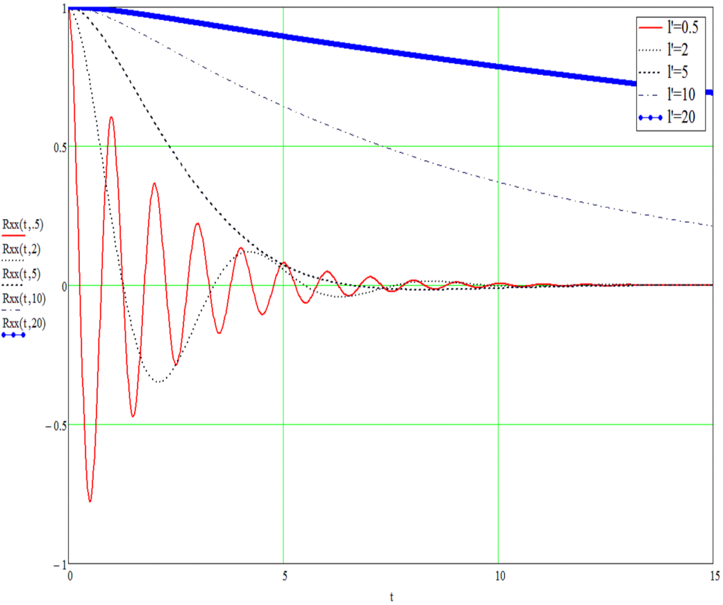
Figure 1: The autocorrelation function for particle position  for particles moving in a rectangular box as a function of dimensionless delay time, $\tau^{\prime},$ with $l^{\prime}=L_{x}/\lambda$, where $L_{x}$ is the length of the cell in the $x$ direction and $\lambda$ is the mean free path between collisions, as a parameter.

Figure 1) shows a plot of $R_{xx}(\tau^{\prime})/R_{xx}(0)$ for various values of $l^{\prime}$.

III.2 Spectrum of the correlation functions.

We start with the velocity auto-correlation function equation (21) and take the Fourier transform of (22) using the definition of Fourier integral used by McGregor McG :

$$\psi_{n}\left(\omega\right)=\int_{-\infty}^{\infty}\psi_{n}\left(\tau\right)e^{=i\omega\tau}d\tau$$ (31)

so that

$$\psi_{n}\left(\omega\right)=2\frac{\omega^{2}}{\tau_{c}}\frac{1}{\left(\omega^{2}-\omega_{n}^{2}\right)^{2}+\omega^{2}/\tau_{c}^{2}}$$ (32)

and following (21)

$$\psi\left(\omega\right)=\frac{8v_{i}^{2}}{\tau_{w}^{2}}{\displaystyle\sum\limits_{n=1,3,5..}}\left[\frac{\psi_{n}\left(\omega\right)}{\omega_{n}^{2}}\right]$$ (33)

Then the spectrum of the position auto-correlation function, $G_{xx}\left(\omega\right)$, which determines the relaxation is given by, following (20)

$$G_{xx}\left(\omega\right) =\frac{\psi\left(\omega\right)}{\omega^{2}}=\frac{16v_{i}^{2}}{\tau_{w}^{2}\tau_{c}}{\displaystyle\sum\limits_{n=1,3,5..}}\left[\frac{1}{\omega_{n}^{2}\left[\left(\omega^{2}-\omega_{n}^{2}\right)^{2}+\omega^{2}/\tau_{c}^{2}\right]}\right]$$ (34)

$$=\frac{16L^{4}}{\lambda v_{i}\pi^{6}}{\displaystyle\sum\limits_{n=1,3,5..}}\frac{1}{n^{6}}\frac{1}{\left[\left(\frac{\omega^{\prime}}{n\pi}\right)^{2}-1\right]^{2}+\left[\frac{\omega^{\prime}l^{\prime}}{\left(n\pi\right)^{2}}\right]^{2}}$$ (35)

where the last equation is written in terms of a normalized frequency, $\omega^{\prime}=\omega L/v_{i}$ and length, $l^{\prime}=L/\lambda.$

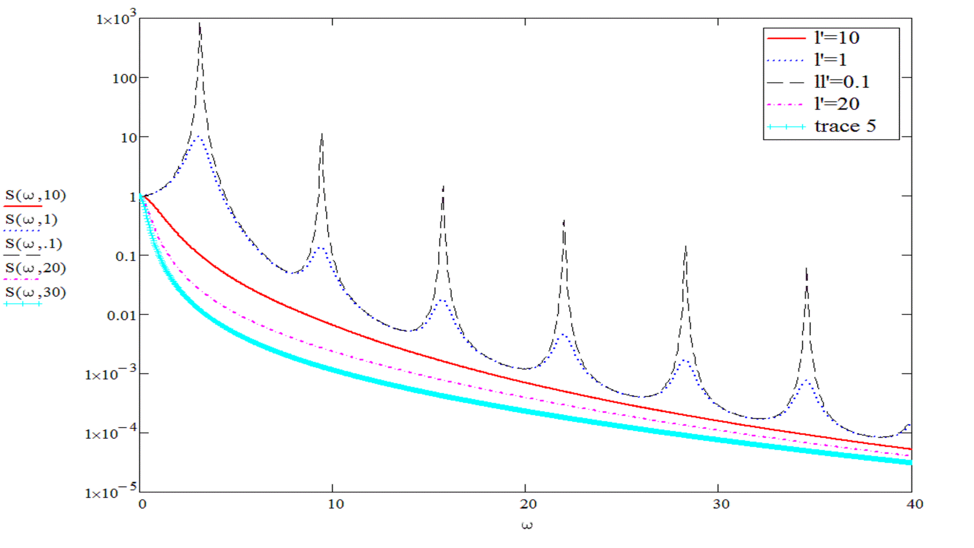
Figure 2: Frequency spectrum of the auto-correlation function of fig.1 as a function of reduced frequency and $l^{\prime}$.

Figure 2) shows $S\left(\omega^{\prime},l^{\prime}\right)=G_{xx}\left(\omega\right)/G_{xx}\left(0\right)$ as a function of $\omega^{\prime}$ with $l^{\prime}$ as a parameter. Note this is for a single velocity. Averaging over the velocity distribution is straightforward.

Taking the limit of (35) for $\omega^{\prime}<<1/\pi$ and reintroducing $\omega,$ we find

$$G_{xx}\left(\omega\right)=16D_{1}{\displaystyle\sum\limits_{n=1,3,5..}}\frac{1}{n^{6}}\frac{1}{\omega^{2}+\left(\frac{\left(n\pi\right)^{2}D_{1}}{L^{2}}\right)^{2}}$$ (36)

where $D_{1}=v_{i}\lambda$ is the diffusion constant for one dimension. This is the Fourier transform of the diffusion theory Green’s function for this problem as obtained by McGregor McG , eqn. (24). For high frequencies, assuming $l^{\prime}$ large, we obtain (neglecting the $1$ in the denominator in (35):

$$G_{xx}\left(\omega\right)=\frac{2v_{i}^{2}\tau_{c}}{\omega^{2}\left(1+\omega^{2}\tau_{c}^{2}\right)}$$ (37)

which is identical to McGregor’s eqn. (13) McG for the high frequency limit. In obtaining equation (37) we assumed

$$\frac{\omega L}{vn\pi}>>1$$

which of course cannot hold for all $n$. This means we are not properly accounting for the high $n$ modes, which in reality would have a contribution of the form (36), which is anyway small for large n, and is responsible for the fact that (37) is independent of the size of the vessel. See the discussion under Fig. 3) in CSH .

IV Discussion

The approaches of the two calculations are quite different. We have seen that Cates, Schaefer and  Happer CSH solved  the Torrey equation (38) by assuming an exponential form for the time dependence of $\rho$ and expanding the decay constant and amplitude in a power series in the fluctuating field, treated as a perturbation. McGregor’s approach is based on the Redfield treatment of the equation of motion for the density matrix, eqn. (38) without the explicit introduction of a diffusion term. Recursion is used to get a second order approximation to this equation and the second order term is written in terms of the correlation functions of the fluctuating field components as seen by the nuclei Sli . The diffusion theory is then introduced in the calculation of these correlation functions. Lastly we have shown that the same results follow from the recursive expansion of the integral equation, derived by use of the Green’s function, in the manner of the Born expansion.

Working out the details of the diffusion theory for a spherical cell McGregor showed that his result is equivalent to that of CSH in the high pressure limit with Neuman boundary conditions. We have shown that the two approaches give identical results whenever eqn. (38) and the perturbation theory is valid, thus clearing up any possible confusion as to when one or the other of the two quite different approaches is valid. The physical content of both theories is identical.

We have also presented a more general form of the position auto-correlation function for the case of a rectangular cell which is valid beyond the region of validity of diffusion theory.

V Acknowledgements

We are grateful to Bradley Fillipone for a helpful remark.

VI
References

VII Appendix A

VII.1 Perturbation theory of Cates, Schaefer and Happer CSH .

The authors start with the equation of motion for the density operator, $\rho$, in diffusion approximation:

$$\frac{\partial\rho}{\partial t}=\frac{1}{i\hslash}\left[H,\rho\right]+D\triangledown^{2}\rho$$ (38)

The Hamiltonian $H$ is broken up into an main term, $H^{(0)}$ and a perturbation $H^{(1)}:$

$$H =H^{(0)}+H^{(1)}$$ (39)

$$H^{(0)} =\hslash\Omega_{o}\sigma_{z}$$ (40)

$$H^{(1)} =\eta\hslash\overrightarrow{\Omega}_{1}\cdot\overrightarrow{\sigma}$$ (41)

where $\Omega_{o}$ is chosen so that the volume average of $\overrightarrow{\Omega}_{1}$ is zero and $\eta$ is an expansion parameter. (Note: normally $\Omega_{o}=\gamma B_{o}$ so here $\Omega_{o,1\text{ }}$are 1/2 the usual values, $\Omega_{o,1\text{ }}=\gamma B_{o,1}/2$)

We rewrite 38 as

$$\frac{\partial\rho}{\partial t}=\frac{1}{i}\left[\Omega_{o}\sigma_{z},\rho\right]+\frac{\eta}{i}\left[\overrightarrow{\Omega}_{1}\cdot\overrightarrow{\sigma},\rho\right]+D\triangledown^{2}\rho$$ (42)

We will approach the problem using time independent perturbation theory, that is we substitute $\rho=\rho^{\prime}e^{-\gamma t}$ and obtain $\left(\rho^{\prime}\neq f(t)\right)$

$$0=\left(\gamma+\frac{1}{i}\Gamma_{o}+D\triangledown^{2}+\frac{\eta}{i}\Gamma_{1}\right)\rho^{\prime}$$ (43)

where $\Gamma_{o,1}$ are linear operators (we now drop the prime on $\rho^{\prime}$, using $\rho$ to indicate the time independent solution)

$$\Gamma_{o}\rho =\left[\Omega_{o}\sigma_{z},\rho\right]$$

$$\Gamma_{1}\rho =\left[\overrightarrow{\Omega}_{1}\cdot\overrightarrow{\sigma},\rho\right]$$ (44)

We will then expand $\rho$ in the spherical components of the spin 1/2 operators $\overrightarrow{\sigma}:$

$$\sigma_{\pm} =\left(\sigma_{x}\pm i\sigma_{y}\right)/2=\sigma_{1,2}$$ (45)

$$\sigma_{0} =\sigma_{z}$$ (46)

The $\sigma_{i}$ are seen to have the following properties

$$Tr(\sigma_{i}^{T}\sigma_{j}) =\delta_{ij}+\delta_{jo}\delta_{io}=\delta_{ij}\alpha_{j}$$ (47)

$$\left[\sigma_{0},\sigma_{i}\right] =\left[\sigma_{z},\sigma_{i}\right]=2M_{i}\sigma_{i}$$ (48)

with $M_{1,2}=\pm 1,M_{0}=0$, and

$$\alpha_{j}=\left\{\begin{array}[c]{c}1\qquad(j=1,2)\\ 2\qquad(j=0)\end{array}\right\}$$ (49)

Thus

$$\Gamma_{o}\sigma_{i}=2\Omega_{o}M_{i}\sigma_{i}$$ (50)

We now follow CSH, CSH , by introducing a perturbation expansion for $\rho(\overrightarrow{r})$ and $\gamma$ into (43)$:$

$$\rho(\overrightarrow{r}) =\rho^{(0)}+\eta\rho^{(1)}+\eta^{2}\rho^{(2)}$$ (51)

$$\gamma =\gamma^{(0)}+\eta\gamma^{(1)}+\eta^{2}\gamma^{(2)}$$ (52)

As this must hold for any value of $\eta$ we collect terms in equal powers of $\eta:$

$$0 =\left(\gamma^{(0)}+\frac{1}{i}\Gamma_{o}+D\triangledown^{2}\right)\rho^{(0)}$$ (53)

$$0 =\left(\gamma^{(0)}+\frac{1}{i}\Gamma_{o}+D\triangledown^{2}\right)\rho^{(1)}+\left(\frac{1}{i}\Gamma_{1}+\gamma^{(1)}\right)\rho^{(0)}$$ (54)

$$0 =\left(\gamma^{(0)}+\frac{1}{i}\Gamma_{o}+D\triangledown^{2}\right)\rho^{(2)}+\left(\frac{1}{i}\Gamma_{1}+\gamma^{(1)}\right)\rho^{(1)}+\gamma^{(2)}\rho^{(0)}$$ (55)

We look for a solution in the form

$$\rho^{(0)}=\sigma_{j}f_{j}^{(0)}(\overrightarrow{r})$$ (56)

Substituting into (53) and applying $Tr(\sigma_{i}^{T}\cdot)$ to the resultant equation yields

$$\left(\gamma_{i}^{(0)}-i2\Omega_{o}M_{i}+D\triangledown^{2}\right)f_{i}^{(0)}(\overrightarrow{r})=0$$ (57)

$f_{i}(\overrightarrow{r})$ has to satisfy boundary conditions on the surface of the measurement cell. CSH, CSH , have taken the von Neuman conditions (zero current at the walls) but as they point out the method can be applied to the case where depolarization takes place at the walls. In any case equation (57), along with the boundary conditions form an eigenvalue problem. The solutions are given by the solution to

$$\left(\triangledown^{2}+k_{\alpha}^{2}\right)\phi_{\alpha}=0$$ (58)

where the eigenvalues $k_{\alpha}$ are determined by the boundary conditions. Then (57) implies

$$\gamma_{i,\alpha}^{(0)}=i2M_{i}\Omega_{o}+Dk_{\alpha}^{2}$$ (59)

In order to solve for the higher order correction terms to the solution it is useful to expand the corrections to $f_{i}(\overrightarrow{r})$ in a series of the zero order functions, $f_{i\alpha}^{(0)}(\overrightarrow{r})=\phi_{i\alpha},$ (the eigenfunctons of (58)).

$$\rho_{i\alpha}^{(n)}(\overrightarrow{r})=\sum_{j\beta^{\prime}}\sigma_{j}\phi_{\beta^{\prime}}a_{j\beta^{\prime},i\alpha}^{(n)}$$ (60)

which form a complete set of functions satisfying the boundary conditions. $n=1$ or $2$ indicates the order of the correction. Thus (54) becomes

$$0 =\left(\gamma_{i,\alpha}^{(0)}+\frac{1}{i}\Gamma_{o}+D\triangledown^{2}\right)\sum_{j,\beta^{\prime}}\sigma_{j}\phi_{\beta^{\prime}}a_{j\beta^{\prime},i\alpha}^{(1)}+\left(\frac{1}{i}\Gamma_{1}+\gamma_{i,\alpha}^{(1)}\right)\sigma_{i}\phi_{\alpha}$$

$$0 =\sum_{j}\left(\gamma_{i,\alpha}^{(0)}+\frac{1}{i}2M_{j}\Omega_{o}+D\triangledown^{2}\right)\sigma_{j}\sum_{\beta^{\prime}}\phi_{\beta^{\prime}}a_{j\beta^{\prime},i\alpha}^{(1)}+\left(\frac{1}{i}\Gamma_{1}+\gamma_{i,\alpha}^{(1)}\right)\sigma_{i}\phi_{\alpha}$$

where we used (50 ). Taking $Tr(\sigma_{g}^{T}\cdot)$ of this last equation yields

$$0=\alpha_{g}\left(\gamma_{i,\alpha}^{(0)}-i2M_{g}\Omega_{o}+D\triangledown^{2}\right)\sum_{\beta^{\prime}}\phi_{g\beta^{\prime}}a_{g\beta^{\prime},i\alpha}^{(1)}+\frac{1}{i}\left[\Gamma_{1}\right]_{g,i}\phi_{\alpha}+\gamma_{i,\alpha}^{(1)}\phi_{\alpha}\delta_{gi}\alpha_{g}$$ (61)

where

$$\left[\Gamma_{1}\right]_{g,i}=Tr(\sigma_{g}^{T}\Gamma_{1}\sigma_{i})=Tr\sigma_{g}^{T}\left[\overrightarrow{\Omega}_{1}\cdot\overrightarrow{\sigma},\sigma_{i}\right]$$ (62)

Making use of the orthogonality of the $\phi_{\alpha},$ and taking them to be normalized

$$\int_{V}d^{3}x\phi_{\beta}^{\ast}\phi_{\alpha}=\delta_{\beta\alpha}$$ (63)

we multiply (61) by $\phi_{\beta}^{\ast}$ and integrate over the volume:

$$0 =\alpha_{g}\left(\gamma_{i,\alpha}^{(0)}-i2M_{g}\Omega_{o}-Dk_{\beta}^{2}\right)a_{g\beta,i\alpha}^{(1)}+\frac{1}{i}\left\langle\beta\right|\left[\Gamma_{1}\right]_{g,i}\left|\alpha\right\rangle+\gamma_{i,\alpha}^{(1)}\delta_{gi}\delta_{\alpha\beta}\alpha_{g}$$

$$0 =\alpha_{g}\left(\gamma_{i,\alpha}^{(0)}-\gamma_{g,\beta}^{(0)}\right)a_{g\beta,i\alpha}^{(1)}+\frac{1}{i}\left\langle\beta\right|\left[\Gamma_{1}\right]_{g,i}\left|\alpha\right\rangle+\gamma_{i,\alpha}^{(1)}\delta_{gi}\delta_{\alpha\beta}\alpha_{g}$$ (64)

using (59), where

$$\left\langle\beta\right|\left[\Gamma_{1}\right]_{i,j}\left|\alpha\right\rangle\triangleq\int_{V}d^{3}x\phi_{\beta}^{\ast}\left[\Gamma_{1}\right]_{i,j}\phi_{\alpha}$$ (65)

We note that $k_{\alpha=0}=0,$ corresponding to a uniform distribution in the cell, is a valid solution and we will seek the decay parameters for this mode. Thus we put $\alpha=\beta=0,$ and $i=g$ in (64) obtaining

$$0 =\frac{1}{i}\left\langle 0\right|\left[\Gamma_{1}\right]_{i,i}\left|0\right\rangle+\gamma_{i,0}^{(1)}\alpha_{i}$$ (66)

$$0 =\gamma_{i,0}^{(1)}$$ (67)

$$a_{g\beta,i0}^{(1)} =\frac{i\left\langle\beta\right|\left[\Gamma_{1}\right]_{g,i}\left|0\right\rangle}{\alpha_{g}\left(\gamma_{i,0}^{(0)}-\gamma_{g,\beta}^{(0)}\right)}$$ (68)

The matrix element in (66) is seen to be zero for perturbing fields with a volume average of zero.

Now we use (55) to evaluate the second order corrections

$$0 =\left(\gamma_{i,\alpha}^{(0)}+\frac{1}{i}\Gamma_{o}+D\triangledown^{2}\right)\sum_{j\beta^{\prime}}\sigma_{j}\phi_{\beta^{\prime}}a_{j\beta^{\prime},i\alpha}^{(2)}+$$

$$\left(\frac{1}{i}\Gamma_{1}+\gamma_{i,\alpha}^{(1)}\right)\sum_{j\beta^{\prime}}\sigma_{j}\phi_{\beta^{\prime}}a_{j\beta^{\prime},i\alpha}^{(1)}+\gamma_{i,\alpha}^{(2)}\sigma_{i}\phi_{\alpha}$$ (69)

Again taking $Tr\left(\sigma_{g}^{\ast}\cdot\right)$ of this equation

$$0 =\alpha_{g}\left(\gamma_{i,\alpha}^{(0)}+\frac{2}{i}M_{g}\Omega_{o}+D\triangledown^{2}\right)\sum_{\beta^{\prime}}\phi_{\beta^{\prime}}a_{g\beta^{\prime},i\alpha}^{(2)}+\sum_{j\beta^{\prime}}\frac{1}{i}\left[\Gamma_{1}\right]_{g,j}\phi_{\beta^{\prime}}a_{j\beta^{\prime},i\alpha}^{(1)}+..$$

$$+\left(\gamma_{i,\alpha}^{(1)}\sum_{\beta^{\prime}}\phi_{\beta^{\prime}}a_{g\beta^{\prime},i\alpha}^{(1)}+\gamma_{i,\alpha}^{(2)}\delta_{gi}\phi_{\alpha}\right)\alpha_{g}$$ (70)

$$0 =\alpha_{g}\left(\gamma_{i,\alpha}^{(0)}-\gamma_{g,\beta}^{(0)}\right)a_{g\beta,i\alpha}^{(2)}+\sum_{j,\beta^{\prime}}\frac{1}{i}\left\langle\beta\right|\left[\Gamma_{1}\right]_{g,j}\left|\beta^{\prime}\right\rangle a_{j\beta^{\prime},i\alpha}^{(1)}+\alpha_{g}\gamma_{i,\alpha}^{(1)}a_{g\beta,i\alpha}^{(1)}+..$$

$$+\gamma_{i,\alpha}^{(2)}\delta_{gi}\delta_{\alpha\beta}\alpha_{g}$$ (71)

where the last result comes from multiplying by $\phi_{\beta}^{\ast}$ and integrating over volume. Now taking $\alpha=\beta=0,i=g,$ we find

$$0 =\sum_{j,\beta^{\prime}}\frac{1}{i}\left\langle 0\right|\left[\Gamma_{1}\right]_{i,j}\left|\beta^{\prime}\right\rangle a_{j\beta^{\prime},i0}^{(1)}+\gamma_{i,0}^{(2)}\alpha_{i}$$

$$\alpha_{i}\gamma_{i,0}^{(2)} =-\sum_{j,\beta^{\prime}}\left\langle 0\right|\left[\Gamma_{1}\right]_{i,j}\left|\beta^{\prime}\right\rangle\frac{\left\langle\beta^{\prime}\right|\left[\Gamma_{1}\right]_{j,i}\left|0\right\rangle}{\left(\gamma_{i,0}^{(0)}-\gamma_{j,\beta^{\prime}}^{(0)}\right)\alpha_{j}}$$ (72)

Our derivation has followed the method of time independent Rayleigh-Schroedinger perturbation theory. The ’states’ are characterized by two ’quantum numbers’ a spin index $i$ and a spatial index $\alpha,$ which can stand for 3 indices, which appear when we solve the diffusion equation in 3 dimensions.

VII.2 Calculation of relaxation times, relation to McGregor’s result

We begin by evaluating (72) for $i=0.$ Since $\sigma_{o}=\sigma_{z}$ this will be equal to $1/T_{1}$. We have then $\left(\phi_{\alpha=0}=1/\sqrt{V}\right)$

$$\left\langle\beta^{\prime}\right|\left[\Gamma_{1}\right]_{j,i}\left|0\right\rangle=\frac{1}{\sqrt{V}}\int d^{3}r\phi_{\beta^{\prime}}\left(\overrightarrow{r}\right)\left[\Gamma_{1}\right]_{j,0}$$ (73)

We write

$$\overrightarrow{\Omega}_{1}\cdot\overrightarrow{\sigma} =\left(\left[\Omega_{1}\right]_{+}\sigma_{-}+\left[\Omega_{1}\right]_{-}\sigma_{+}\right)+\left[\Omega_{1}\right]_{z}\sigma_{z}$$ (74)

$$\left[\overrightarrow{\Omega}_{1}\cdot\overrightarrow{\sigma},\sigma_{o}\right] =2\left(\left[\Omega_{1}\right]_{+}\sigma_{-}-\left[\Omega_{1}\right]_{-}\sigma_{+}\right)$$ (75)

$$\left[\Gamma_{1}\right]_{j,0} =Tr\sigma_{j}^{T}\left[\overrightarrow{\Omega}_{1}\cdot\overrightarrow{\sigma},\sigma_{o}\right]$$ (76)

$$\left[\Gamma_{1}\right]_{-,0} =2\left[\Omega_{1}\right]_{+}$$ (77)

$$\left[\Gamma_{1}\right]_{+,0} =-2\left[\Omega_{1}\right]_{-}$$ (78)

Thus

$$\gamma_{i=0,0}^{(2)} =\frac{1}{T_{1}}=-\frac{1}{\alpha_{o}}\sum_{j,\beta^{\prime}}\left\langle 0\right|\left[\Gamma_{1}\right]_{0,j}\left|\beta^{\prime}\right\rangle\frac{\left\langle\beta^{\prime}\right|\left[\Gamma_{1}\right]_{j,0}\left|0\right\rangle}{\left(\gamma_{0,0}^{(0)}-\gamma_{j,\beta^{\prime}}^{(0)}\right)\alpha_{j}}$$

$$=\frac{4}{V\alpha_{o}}\int\int\left[\Omega_{1}\left(\overrightarrow{r^{\prime}}\right)\right]_{-}\left[\Omega_{1}\left(\overrightarrow{r}\right)\right]_{+}\sum_{\beta^{\prime}}\ \left(\frac{\phi_{\beta^{\prime}}\left(\overrightarrow{r^{\prime}}\right)\phi_{\beta^{\prime}}\left(\overrightarrow{r}\right)}{(Dk_{\beta^{\prime}}^{2}-i2\Omega_{o})}\right)d^{3}r^{\prime}d^{3}r$$

$$+cc$$

$$\frac{1}{T_{1}} =\frac{4}{V}\operatorname{Re}\int\int\left[\Omega_{1}\left(\overrightarrow{r^{\prime}}\right)\right]_{-}\left[\Omega_{1}\left(\overrightarrow{r}\right)\right]_{+}\sum_{\beta^{\prime}}\ \left(\frac{\phi_{\beta^{\prime}}\left(\overrightarrow{r^{\prime}}\right)\phi_{\beta^{\prime}}\left(\overrightarrow{r}\right)}{(Dk_{\beta^{\prime}}^{2}-i2\Omega_{o})}\right)d^{3}r^{\prime}d^{3}r$$

(79)

Now the Green’s function for the diffusion equation can be written (see Morse and Feshbach, [MandF ] chapter 7)

$$G\left(\overrightarrow{r},t|\overrightarrow{r}^{\prime},t^{\prime}\right)=u\left(t-t^{\prime}\right)\sum_{\beta}\phi_{\beta}\left(\overrightarrow{r^{\prime}}\right)\phi_{\beta}\left(\overrightarrow{r}\right)e^{-Dk_{\beta}^{2}(t-t^{\prime})}$$ (80)

with $u\left(t\right),$ the unit step function. Then the time Fourier transform is $\left(\tau=t-t^{\prime}\right)$

$$\widetilde{G}\left(\overrightarrow{r},\overrightarrow{r}^{\prime},\omega\right) =\int_{0}^{\infty}d\tau e^{i\omega\tau}G\left(\overrightarrow{r},t|\overrightarrow{r}^{\prime},t^{\prime}\right)$$ (81)

$$=\int_{0}^{\infty}d\tau e^{i\omega\tau}\sum_{\beta}\phi_{\beta}\left(\overrightarrow{r^{\prime}}\right)\phi_{\beta}\left(\overrightarrow{r}\right)e^{-Dk_{\beta}^{2}\tau}$$ (82)

$$=\sum_{\beta^{\prime}}\ \left(\frac{\phi_{\beta^{\prime}}\left(\overrightarrow{r^{\prime}}\right)\phi_{\beta^{\prime}}\left(\overrightarrow{r}\right)}{(Dk_{\beta^{\prime}}^{2}-i\omega)}\right)$$ (83)

Comparing to the sum in (79) we see that we can write $\left(\alpha_{0}=2\right)$

$$\frac{1}{T_{1}} =\operatorname{Re}\gamma_{i=0,0}^{(2)}$$

$$=\frac{4\operatorname{Re}}{V}\int\int\left[\Omega_{1}\left(\overrightarrow{r^{\prime}}\right)\right]_{-}\left[\Omega_{1}\left(\overrightarrow{r}\right)\right]_{+}\widetilde{G}\left(\overrightarrow{r},\overrightarrow{r}^{\prime},2\Omega_{o}\right)d^{3}r^{\prime}d^{3}r$$

$$=4\frac{\operatorname{Re}}{V}\int_{0}^{\infty}d\tau e^{i2\Omega_{o}\tau}\int\int\left[\Omega_{1}\left(\overrightarrow{r^{\prime}}\right)\right]_{-}\left[\Omega_{1}\left(\overrightarrow{r}\right)\right]_{+}G\left(\overrightarrow{r},t|\overrightarrow{r}^{\prime},t^{\prime}\right)d^{3}r^{\prime}d^{3}r$$

$$=4\operatorname{Re}\int_{0}^{\infty}d\tau e^{i\omega_{o}\tau}\int\int\left[\Omega_{1}\left(\overrightarrow{r^{\prime}}\right)\right]_{-}\left[\Omega_{1}\left(\overrightarrow{r}\right)\right]_{+}G\left(\overrightarrow{r},t|\overrightarrow{r}^{\prime},t^{\prime}\right)p_{o}(r^{\prime},t^{\prime})d^{3}r^{\prime}d^{3}r$$

(84)

Where $\omega_{o}=\gamma B_{o}$ and $p_{o}(r^{\prime},t^{\prime})=1/V$ is the uniform density of magnetization. Then the joint probability distribution of an atom being at $\overrightarrow{r}$ at time $t$ and being at $\overrightarrow{r}^{\prime}$ at time $t^{\prime}$ is $G\left(\overrightarrow{r},t|\overrightarrow{r}^{\prime},t^{\prime}\right)p_{o}(r^{\prime},t^{\prime})$ and we see that (following McGregor’s notation)

$$\frac{1}{T_{1}} =\gamma_{i=0,0}^{(2)}=4\operatorname{Re}\int_{0}^{\infty}d\tau e^{i\omega_{o}\tau}\left\langle\left[\Omega_{1}\left(t\right)\right]_{-}\left[\Omega_{1}\left(t+\tau\right)\right]_{+}\right\rangle$$

$$=4\int_{0}^{\infty}d\tau e^{i\omega_{o}\tau}\left\langle\left[\Omega_{1}\left(t\right)\right]_{x}\left[\Omega_{1}\left(t+\tau\right)\right]_{x}+\left[\Omega_{1}\left(t\right)\right]_{y}\left[\Omega_{1}\left(t+\tau\right)\right]_{y}\right\rangle$$

$$=\frac{\gamma^{2}}{2}\int_{-\infty}^{\infty}d\tau e^{i\omega_{o}\tau}\left\langle\left[B_{1}\right]_{x}\left[B_{1}\left(t+\tau\right)\right]_{x}+\left[B_{1}\left(t\right)\right]_{y}\left[B_{1}\left(t+\tau\right)\right]_{y}\right\rangle$$ (85)

This is the result of the Redfield theory given as equation (9) in McGregor.

To calculate $T_{2}$ we have to evaluate $\gamma_{i=+,0}^{(2)}.$

$$\gamma_{i=+,0}^{(2)}=-\sum_{j,\beta^{\prime}}\left\langle 0\right|\left[\Gamma_{1}\right]_{+,j}\left|\beta^{\prime}\right\rangle\frac{\left\langle\beta^{\prime}\right|\left[\Gamma_{1}\right]_{j,+}\left|0\right\rangle}{\left(\gamma_{+,0}^{(0)}-\gamma_{j,\beta^{\prime}}^{(0)}\right)\alpha_{j}}$$ (86)

The non-zero matrix elements are

$$\left[\Gamma_{1}\right]_{+,+} =2\left[\Omega_{1}\right]_{z}$$ (87)

$$\left[\Gamma_{1}\right]_{o,+} =-2\left[\Omega_{1}\right]_{+}$$ (88)

so that

$$\gamma_{i=+,0}^{(2)} =\frac{1}{T_{2}}=-\operatorname{Re}\sum_{\beta^{\prime}}\left[\begin{array}[c]{c}\left\langle 0\right|\left[\Gamma_{1}\right]_{+,+}\left|\beta^{\prime}\right\rangle\frac{\left\langle\beta^{\prime}\right|\left[\Gamma_{1}\right]_{+,+}\left|0\right\rangle}{\left(\gamma_{+,0}^{(0)}-\gamma_{+,\beta^{\prime}}^{(0)}\right)}+\\ \left\langle 0\right|\left[\Gamma_{1}\right]_{+,0}\left|\beta^{\prime}\right\rangle\frac{\left\langle\beta^{\prime}\right|\left[\Gamma_{1}\right]_{0,+}\left|0\right\rangle}{2\left(\gamma_{+,0}^{(0)}-\gamma_{0,\beta^{\prime}}^{(0)}\right)}\end{array}\right]$$ (91)

$$=-\operatorname{Re}\sum_{\beta^{\prime}}\left[\begin{array}[c]{c}4\frac{\left\langle 0\right|\left[\Omega_{1}\right]_{z}\left|\beta^{\prime}\right\rangle\left\langle\beta^{\prime}\right|\left[\Omega_{1}\right]_{z}\left|0\right\rangle}{\left(\gamma_{+,0}^{(0)}-\gamma_{+,\beta^{\prime}}^{(0)}\right)}+\\ 4\frac{\left\langle 0\right|\left[\Omega_{1}\right]_{-}\left|\beta^{\prime}\right\rangle\left\langle\beta^{\prime}\right|\left[\Omega_{1}\right]_{+}\left|0\right\rangle}{2\left(\gamma_{+,0}^{(0)}-\gamma_{0,\beta^{\prime}}^{(0)}\right)}\end{array}\right]$$ (94)

$$=4\operatorname{Re}\sum_{\beta^{\prime}}\left[\frac{\left\langle 0\right|\left[\Omega_{1}\right]_{z}\left|\beta^{\prime}\right\rangle\left\langle\beta^{\prime}\right|\left[\Omega_{1}\right]_{z}\left|0\right\rangle}{\left(Dk_{\beta^{\prime}}^{2}\right)}+\frac{\left\langle 0\right|\left[\Omega_{1}\right]_{-}\left|\beta^{\prime}\right\rangle\left\langle\beta^{\prime}\right|\left[\Omega_{1}\right]_{+}\left|0\right\rangle}{2\left(Dk_{\beta^{\prime}}^{2}-i\omega_{o}\right)}\right]$$

$$\frac{1}{T_{2}} =\frac{4\operatorname{Re}}{V}\int\int\left[\Omega_{1}\left(\overrightarrow{r^{\prime}}\right)\right]_{z}\left[\Omega_{1}\left(\overrightarrow{r}\right)\right]_{z}\sum_{\beta^{\prime}}\ \left(\frac{\phi_{\beta^{\prime}}\left(\overrightarrow{r^{\prime}}\right)\phi_{\beta^{\prime}}\left(\overrightarrow{r}\right)}{Dk_{\beta^{\prime}}^{2}}\right)d^{3}r^{\prime}d^{3}r+$$

$$\frac{2\operatorname{Re}}{V}\int\int\left[\Omega_{1}\left(\overrightarrow{r^{\prime}}\right)\right]_{-}\left[\Omega_{1}\left(\overrightarrow{r}\right)\right]_{+}\sum_{\beta^{\prime}}\ \left(\frac{\phi_{\beta^{\prime}}\left(\overrightarrow{r^{\prime}}\right)\phi_{\beta^{\prime}}\left(\overrightarrow{r}\right)}{(Dk_{\beta^{\prime}}^{2}-i\omega_{o})}\right)d^{3}r^{\prime}d^{3}r$$

(95)

From (83) we write

$$\widetilde{G}\left(\overrightarrow{r},\overrightarrow{r}^{\prime},\omega=0\right) =\sum_{\beta^{\prime}}\ \left(\frac{\phi_{\beta^{\prime}}\left(\overrightarrow{r^{\prime}}\right)\phi_{\beta^{\prime}}\left(\overrightarrow{r}\right)}{Dk_{\beta^{\prime}}^{2}}\right)$$

$$=\int_{0}^{\infty}d\tau G\left(\overrightarrow{r},t|\overrightarrow{r}^{\prime},t^{\prime}\right)$$ (96)

so that the first term in (95) can be written

$$\frac{\gamma^{2}\operatorname{Re}}{2}\int_{-\infty}^{\infty}d\tau\int\int\left[B_{1}\left(\overrightarrow{r^{\prime}}\right)\right]_{z}\left[B_{1}\left(\overrightarrow{r}\right)\right]_{z}G\left(\overrightarrow{r},t|\overrightarrow{r}^{\prime},t+\tau\right)p_{o}\left(r^{\prime}\right)d^{3}r^{\prime}d^{3}r$$

$$=\frac{\gamma^{2}}{2}\int_{-\infty}^{\infty}d\tau\left\langle\left[B_{1}\left(t\right)\right]_{z}\left[B_{1}\left(t+\tau\right)\right]_{z}\right\rangle$$ (97)

in agreement with the second term in equ (10) of McGregor.

From (79) we see that the second term is $1/2T_{1}$ so that equation (95) is equivalent to

$$\frac{1}{T_{2}}=\frac{1}{2T_{1}}+\frac{\gamma^{2}}{2}\int_{-\infty}^{\infty}d\tau\left\langle\left[B_{1}\left(t\right)\right]_{z}\left[B_{1}\left(t+\tau\right)\right]_{z}\right\rangle$$ (98)

which is equivalent to equation (10) of McG .

VIII Appendix B, spin relations and matrix elements

$\left[\sigma_{1},\sigma_{z}\right]=-2\sigma_{1}\qquad\left[\sigma_{2},\sigma_{z}\right]=2\sigma_{2}\qquad\left[\sigma_{1},\sigma_{2}\right]=\sigma_{z}$

$$\overrightarrow{\Omega}_{1}\cdot\overrightarrow{\sigma} =\left[\Omega_{1}\right]_{+}\sigma_{-}+\left[\Omega_{1}\right]_{-}\sigma_{+}+\left[\Omega_{1}\right]_{z}\sigma_{z}\qquad\ \left(\sigma_{\pm}=\frac{1}{2}\left(\sigma_{x}\pm i\sigma_{y}\right)\right)$$ (99)

$$\left[\overrightarrow{\Omega}_{1}\cdot\overrightarrow{\sigma},\sigma_{z}\right] =2\left(\left[\Omega_{1}\right]_{+}\sigma_{-}-\left[\Omega_{1}\right]_{-}\sigma_{+}\right)$$ (100)

$$\left[\Gamma_{1}\right]_{g.i} =Tr\left(\sigma_{g}^{T}\left[\overrightarrow{\Omega}_{1}\cdot\overrightarrow{\sigma},\sigma_{i}\right]\right)$$ (101)

$$\left[\Gamma_{1}\right]_{+.z} =-2\left[\Omega_{1}\right]_{-}\qquad\left[\Gamma_{1}\right]_{-.z}=2\left[\Omega_{1}\right]_{+}$$ (102)

$$\left[\overrightarrow{\Omega}_{1}\cdot\overrightarrow{\sigma},\sigma_{+}\right] =-\left[\Omega_{1}\right]_{+}\sigma_{z}+\left[\Omega_{1}\right]_{z}2\sigma_{+}$$ (103)

$$\left[\Gamma_{1}\right]_{z,+} =-2\left[\Omega_{1}\right]_{+}\qquad\left[\Gamma_{1}\right]_{+,+}=2\left[\Omega_{1}\right]_{z}$$ (104)

$$\left[\overrightarrow{\Omega}_{1}\cdot\overrightarrow{\sigma},\sigma_{-}\right] =\left[\Omega_{1}\right]_{-}\sigma_{z}-\left[\Omega_{1}\right]_{z}2\sigma_{-}$$ (105)

$$\left[\Gamma_{1}\right]_{z,-} =2\left[\Omega_{1}\right]_{-}\qquad\left[\Gamma_{1}\right]_{-,-}=-2\left[\Omega_{1}\right]_{z}$$ (106)

Note

$$\sum_{n=0}^{\infty}\frac{1}{\left(2n+1\right)^{4}} =\frac{1}{96}\pi^{4}$$ (107)

$$\sum_{n=0}^{\infty}\frac{1}{\left(2n+1\right)^{6}} =\allowbreak\frac{1}{960}\pi^{6}$$ (108)

$$\sum_{n=0}^{\infty}\frac{1}{\left(2n+1\right)^{2}} =\allowbreak\frac{1}{8}\pi^{2}$$ (109)

References

- (1) A.R. Petukhov, G. Pignol, D. Jullien and K.H. Andersen, arXiv:1009.3434v2 [physics.atom-ph] (2010)
- (2) Yu.N. Pokotilovski, Physics Letters B686, 114 (2010)
- (3) E.L.Hahn, Phys. Rev 80, 580 (1950)
- (4) H.C. Torrey, Phys. Rev. 92, 962 (19530
- (5) H.Y. Carr and E.M. Purcell, Phys. Rev. 94, 630 (1954)
- (6) H.C. Torrey, Phys. Rev. 104, 563, (1956).
- (7) B. Robertson, Phys. Rev, 151, 273, (1966)
- (8) C.H. Neuman, J. Chem. Phys. 60, 4508 (1974)
- (9) G.D. Cates, S.R. Schaefer and W. Happer Phys. Rev. A 37, 2877, (1988)
- (10) D.D. McGregor Phys. Rev. A 41, 2631, (1990)
- (11) A.G. Redfield, IBM Journal of Research and Development, 1,15, (1957)
- (12) C.P. Slichter ”Principles of Magnetic Resonance”, Harper and Row, New York (1963)
- (13) S.D. Stoller, W. Happer and F.J. Dyson, Phys. Rev. A44, 7459 (1991)
- (14) T.M. de Swiet and P.N. Sen, J. Chem. Phys, 100, 5597 (1994)
- (15) M.E. Hayden, G. Archibald, K.M. Gilbert and C. Lei, J Magn. Res. 169, 313, (2004)
- (16) A. Papoulis, Probability, Random Variables and Stochastic Processes, McGraw-Hill. New York (1965)
- (17) A.L. Barabanov, R. Golub and S.K. Lamoreaux, Phys. Rev. A 74, 052115 (2006)
- (18) R. Golub, C.M. Swank and S.K. Lamoreaux, . arXiv:0810.5378 (2009)
- (19) S.K. Lamoreaux and R. Golub, Phys. Rev. A71, 032104, (2005)
- (20) P.M. Morse and H. Feshbach, ”Methods of Theoretical Physic” McGraw-Hill (1953)