Revisiting the Phase Transition of Spin-1/2 Heisenberg Model with a Spatially Staggered Anisotropy on the Square Lattice
Abstract
Puzzled by the indication of a new critical theory for the spin-1/2 Heisenberg model with a spatially staggered anisotropy on the square lattice as suggested in Wenzel08 , we re-investigate the phase transition of this model induced by dimerization using first principle Monte Carlo simulations. We focus on studying the finite-size scaling of and , where stands for the spatial box size used in the simulations and with is the spin-stiffness in -direction. From our Monte Carlo data, we find that suffers a much less severe correction compared to that of . Therefore is a better quantity than for finite-size scaling analysis concerning the limitation of the availability of large volumes data in our study. Further, motivated by the so-called cubical regime in magnon chiral perturbation theory, we additionally perform a finite-size scaling analysis on our Monte Carlo data with the assumption that the ratio of spatial winding numbers squared is fixed through all simulations. As a result, the physical shape of the system remains fixed in our calculations. The validity of this new idea is confirmed by studying the phase transition driven by spatial anisotropy for the ladder anisotropic Heisenberg model. With this new strategy, even from which receives the most serious correction among the observables considered in this study, we arrive at a value for the critical exponent which is consistent with the expected value by using only up to data points.
I Introduction
Heisenberg-type models have been studied in great detail during the last twenty years because of their phenomenological importance. For example, it is believed that the spin-1/2 Heisenberg model on the square lattice is the correct model for understanding the undoped precursors of high cuprates (undoped antiferromagnets). Further, due to the availability of efficient Monte Carlo algorithms as well as the increasing power of computing resources, properties of undoped antiferromagnets on geometrically non-frustrated lattices have been determined to unprecedented accuracy Sandvik97 ; Sandvik99 ; Kim00 ; Wang05 ; Jiang08 ; Alb08 ; Wenzel09 . For instance, using a loop algorithm, the low-energy parameters of the spin-1/2 Heisenberg model on the square lattice are calculated very precisely and are in quantitative agreement with the experimental results Wie94 . Despite being well studied, several recent numerical investigation of anisotropic Heisenberg models have led to unexpected results Wenzel08 ; Pardini08 ; Jiang09.1 . In particular, Monte Carlo evidence indicates that the anisotropic Heisenberg model with staggered arrangement of the antiferromagnetic couplings may belong to a new universality class, in contradiction to the theoretical universality prediction Wenzel08 . For example, while the most accurate Monte Carlo value for the critical exponent in the universality class is given by Cam02 , the corresponding determined in Wenzel08 is shown to be . Although subtlety of calculating the critical exponent from performing finite-size scaling analysis is demonstrated for a similar anisotropic Heisenberg model on the honeycomb lattice Jiang09.2 , the discrepancy between and observed in Wenzel08 ; Cam02 remains to be understood.
In order to clarify this issue further, we have simulated the spin-1/2 Heisenberg model with a spatially staggered anisotropy on the square lattice. Further, we choose to analyze the finite-size scaling of the observables and , where refers to the box size used in the simulations and with is the spin stiffness in -direction. The reason for choosing and is twofold. First of all, these two observables can be calculated to a very high accuracy using loop algorithms. Secondly, one can measure and separately. In practice, one would naturally use which is the average of and for the data analysis. However for the model considered here, we find it is useful to analyze both the data of and because studying and individually might reveal the impact of anisotropy on the system. Surprisingly, as we will show later, the observable receives a much less severe correction than does. Hence is a better observable than (or ) for finite-size scaling analysis concerning the limitation of the availability of large volumes data in this study. Further, motivated by the so-called cubical regime in magnon chiral perturbation theory, we have performed an additional finite-size scaling analysis on with the assumption that the ratio of spatial winding numbers squared is fixed in all our Monte-Carlo simulations. In other word, we keep the physical shape of the system fixed in the additional analysis of finite-size scaling. The validity of this new idea is confirmed by studying the phase transition driven by spatial anisotropy for the ladder anisotropic Heisenberg model, namely the critical point and critical exponent for this phase transition we obtain by fixing the ratio of spatial winding numbers squared are consistent with the known results in the literature. Remarkably, combining the idea of fixing the ratio of spatial winding numbers squared in the simulations and finite-size scaling analysis, unlike the unconventional value for observed in Wenzel08 , even from which suffers a very serious correction, we arrive at a value for which is consistent with that of by using only up to data points.
This paper is organized as follows. In section II, the anisotropic Heisenberg model and the relevant observables studied in this work are briefly described. Section III contains our numerical results. In particular, the corresponding critical point as well as the critical exponent are determined by fitting the numerical data to their predicted critical behavior near the transition. Finally, we conclude our study in section IV.

II Microscopic Model and Corresponding Observables
The Heisenberg model considered in this study is defined by the Hamilton operator
| (1) |
where and are antiferromagnetic exchange couplings connecting nearest neighbor spins and , respectively. Figure 1 illustrates the Heisenberg model described by Eq. (1). To study the critical behavior of this anisotropic Heisenberg model near the transition driven by spatial anisotropy, in particular to determine the critical point as well as the critical exponent , the spin stiffnesses in - and -directions which are defined by
| (2) |
are measured in our simulations. Here is the inverse temperature and refers to the spatial box size. Further with is the winding number squared in -direction. By carefully investigating the spatial volumes and the dependence of , one can determine the critical point as well as the critical exponent with high precision.
III Determination of the Critical Point and the Critical Exponent
To calculate the relevant critical exponent and to determine the location of the critical point in the parameter space , one useful technique is to study the finite-size scaling of certain observables. For example, if the transition is second order, then near the transition, the observable for should be described well by the following finite-size scaling ansatz
| (3) |
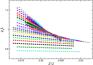
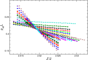
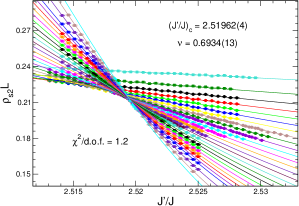
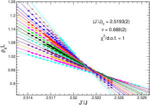
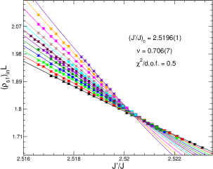
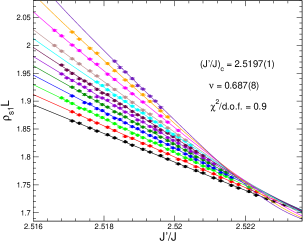
where stands for , is the physical linear length of the system, with , is some constant, is the critical exponent corresponding to the correlation length and is the confluent correction exponent. Finally appearing above is a smooth function of the variable . In practice, the appearing in Eq. (3) is conventionally replaced by the box size used in the simulations when performing finite-size scaling analysis. We will adopt this conventional strategy in the first part of our analysis as well. From Eq. (3), one concludes that the curves of different for , as functions of , should have the tendency to intersect at critical point for large . To calculate the critical exponent and the critical point , in the following we will apply the finite-size scaling formula, Eq. (3), to both and . Without losing the generality, in our simulations we have fixed to be and have varied . Further, the box size used in the simulations ranges from to . We also use large enough so that the observables studied here take their zero-temperature values. Figure 2 shows the Monte Carlo data of and as functions of the parameter . The figure clearly indicates the phase transition is likely second order since different curves for both and tend to intersect at a particular point in the parameter space . What is the most striking observation from our results is that the observable receives a much severe correction than does. This can be understood from the trend of the crossing among these curves of different in figure 2. Therefore one expects a better determination of can be obtained by applying finite-size scaling analysis to . Before presenting our results, we would like to point out that since data from large volumes might be essential in order to determine the critical exponent accurately as suggested in Jiang09.2 , we will use the strategy employed in Jiang09.2 for our data analysis as well. A Taylor expansion of Eq. (3) up to fourth order in is used to fit the data of . The critical exponent and critical point calculated from the fit using all the available data of are given by and , respectively. The upper panel of figure 3 demonstrates the result of the fit. Notice both and we obtain are consistent with the corresponding results found in Wenzel08 . By eliminating some data points of small , we can reach a value of for by fitting with to Eq. (3). On the other hand, with the same range of (), a fit of to Eq. (3) leads to and , both of which are consistent with those obtained in Wenzel08 as well (lower panel in figure 3). By eliminating more data points of with small , the values for and calculated from the fits are always consistent with those quoted above. What we have shown clearly indicates that one would suffer the least correction by considering the finite-size scaling of the observable . As a result, it is likely one can reach a value for consistent with the prediction, namely if large volume data points for are available. Here we do not attempt to carry out such task of obtaining data for . Instead, we employ the technique of fixing the ratio of spatial winding numbers squared in the simulations. Surprisingly, combining this new idea and finite-size scaling analysis, even from the observable which is found to receive the most severe correction among the observables considered here, we reach a value for the critical exponent consistent with without additionally obtaining data points for . The motivation behind the idea of fixing the ratio of spatial winding numbers squared in the simulations is as follows. First of all, as we already mentioned earlier that the box size used in the simulations is conventionally used as the in Eq. (3) when carrying out finite-size scaling analysis. For isotropic systems, such strategy is no problem. However, for anisotropic cases, the validity of this common wisdom of treating as is not clear. In particular, the same does not stand for the same of the system for two different anisotropies . Hence one needs to find a physical quantity which can really characterize the physical linear length of the system. Secondly, in magnon chiral perturbation theory which is the low-energy effective field theory for spin-1/2 antiferromagnets with symmetry, an exactly cubical space-time box is met when the condition is satisfied, here is the spin-wave velocity and , are the inverse temperature and box size as before. For spin-1/2 XY model on the square lattice, for large box size , the numerical value of c determined by using the with which one obtains in the Monte Carlo simulations agrees quantitatively with the known results in the literature Jiang10.1 . This result implies that the squares of winding numbers are more physical than the box sizes since an exactly cubical space-time box is reached when the squares of spatial and temporal winding numbers are tuned to be the same in the Monte Carlo simulations. Consequently the physical linear lengths of the system should be characterized by the squares of winding numbers, not the box sizes used in the simulations. Based on what we have argued, it is , not , plays the role of the quantity for the system, here again we refer with as the physical linear length of the system in -direction. As a result, fixing the ratio of spatial winding numbers squared in the simulations corresponds to the situation that the physical shape of the system remains fixed in all calculations. Indeed it is demonstrated in Sandvik99 that rectangular lattice is more suitable than square lattice for studying the spatially anisotropic Heisenberg model with different antiferromagnetic couplings , in 1- and 2-directions. The idea of fixing the ratio of spatial winding numbers squared quantifies the method used in Sandvik99 .
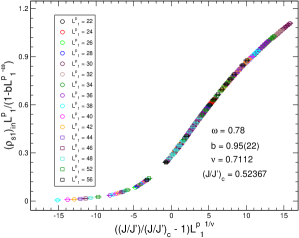
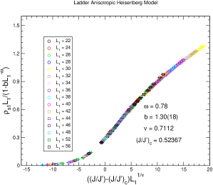
The method of fixing the ratio of spatial winding numbers squared is employed as follows. First of all, we perform a trial simulation to determine a fixed value for the ratio of spatial winding numbers squared which we denote by and will be used later in all calculations. Secondly, instead of fixing the aspect ratio of box sizes and in the simulations as in conventional finite-size scaling studies, we vary the variables , and in order to satisfy the condition of a fixed ratio of spatial winding numbers squared. This step involves a controlled interpolation on the raw data points. In practice, for a fixed one performs simulations for a sequence . The criterion of a fixed ratio of spatial winding numbers squared is reached by tuning the parameter and then carrying out a linear interpolation based on for the desired observables, here refers to the ratio of spatial winding numbers squared of the data points other than the trial one. Notice since only the ratio of the physical linear lengths squared is fixed, it is natural to use in the finite-size scaling ansatz Eq. (3) both for the analysis of and . The validity of this unconventional finite-size scaling method can be verified by considering the transition induced by dimerization for the Heisenberg model with a ladder pattern anisotropic couplings (figure 4). For in Eq. (3), we obtain a good data collapse for the observable . Above the subscript “in” means the data points are the interpolated one. To make sure that the step of interpolation leads to accurate results, we have carried out several trial simulations and have confirmed that the interpolated data points are reliable as long as the ratio is kept small (table 1). On the other hand, for in Eq. (3), a good data collapse is also obtained for the observable , here are the raw data determined from the simulations directly. Figure 5 shows a comparison between the data collapse obtained by using the new unconventional method introduced above (upper panel) and by the conventional method (lower panel). For obtaining figure 5, we have fixed , , and , which are the established values for these quantities. As one sees in figure 5, the quality of the data collapse obtained with the new method is better than the one obtained with the conventional method, thus confirming the validity of the idea to fix the ratio of winding numbers squared in order to studying the critical theory of a second order phase transition.
| 0.53 | 96 | 96 | 0.9558(33) | 0.008188(22) | 0.008198(7) |
| 0.53 | 96 | 94 | 0.9549(32) | 0.008391(21) | 0.0084098(74) |
| 0.545 | 90 | 94 | 0.9594(35) | 0.016862(33) | 0.016835(15) |
| 0.545 | 90 | 90 | 0.9539(36) | 0.017651(35) | 0.017676(17) |
| 0.535 | 98 | 98 | 0.9591(28) | 0.011707(28) | 0.0117297(124) |
| 0.54 | 96 | 96 | 0.9592(29) | 0.014838(37) | 0.014846(13) |
| 0.525 | 96 | 96 | 0.9503(41) | 0.0072255(225) | 0.0072579(66) |

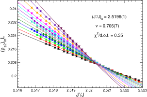
As demonstrated above, in general for a fixed , one can vary and in order to reach the criterion of a fixed aspect-ratio of spatial winding numbers squared in the simulations. For our study here, without obtaining additional data, we proceed as follows. First of all, we calculate the ratio for the data point at and which we denote by . We further choose in our data analysis. After obtaining this number, a linear interpolation for of other data points based on is performed in order to reach the criterion of a fixed ratio of spatial winding numbers squared in the simulations. The appearing above is again the corresponding of other data points. Here a controlled interpolation similar to what we have done in studying the ladder anisotropic Heisenberg model is performed as well. Further, since large volumes data is essential for a quick convergence of as suggested in Jiang09.2 , we make sure the set of interpolated data chosen for finite-size scaling analysis contains sufficiently many points from large volumes as long as the interpolated results are reliable. A fit of the interpolated data to Eq. (3) with being fixed to its value () leads to and for (figure 5). Letting be a fit parameter results in consistent and . Further, we always arrive at consistent results with and from the fits using data. The value of we calculate from the fit is in good agreement with the expected value . The critical point is consistent with that found in Wenzel08 as well. To avoid any bias, we perform another analysis for the raw data with the same range of and as we did for the interpolated data. By fitting this set of original data points to Eq. (3) with a fixed , we arrive at and (figure 6), both of which again agree quantitatively with those determined in Wenzel08 . Similarly, applying this unconventional finite-size scaling to would lead to a numerical value of consistent with . For instance, the determined by fitting to Eq. (3) is found to be , which agrees quantitatively with the predicted value (figure 8). Finally we would like to make a comment regarding the choice of . In principle one can use determined from any and from any close to . However it will be desirable to choose such that the set of interpolated data used for analysis includes as many data points from large volumes as possible. Using the obtained at () with (), we reach the results of and ( and ) from the fit with a fixed . These values for and agree with what we have obtained earlier. Indeed as we will demonstrate in another investigation, the critical exponent determined by the idea of fixing the ratio of spatial winding number squared in the simulations is independence of the chosen reference point.
IV Discussion and Conclusion
In this paper, we revisit the phase transition driven by dimerization for the spin-1/2 Heisenberg model with a spatially staggered anisotropy on the square lattice. We find that the observable suffers a much less severe correction compared to that of , hence is a better quantity for finite-size scaling analysis. Further, we propose an unconventional finite-size scaling method, namely we fix the ratio of spatial winding numbers squared. As a result, the physical shape of the system remains fixed in all simulations and analysis. With this new strategy, we arrive at for the critical exponent which is consistent with the most accurate Monte Carlo result by using only up to data points derived from both and . Interestingly, the obtained from the fits using the interpolated data are better than those resulted from the fits using the raw data (figures 6, 7 and 8). This observation provides another evidence to support the quantitative correctness of the new unconventional finite-size scaling we proposed here.
It seems that when carrying out the finite-size scaling analysis for the observables considered here, the use of physical linear lengths of the system, which are charaterized by the spatial winding numbers squared, would lead to a faster convergence of . It will be interesting to apply a similar technique to other observables such as Binder cumulants as well. However, for Binder cumulants, the correction from interpolation will cancel out because of the definition of these observables. Therefore to further test the philosophy behind the unconventional finite-size scaling method proposed here might require some new ideas. Nevertheless, with this new unconventional finite-size scaling method, we have successfully solved the puzzle raised in Wenzel08 by showing that the anisotropy driven phase transition for the spin-1/2 Heisenberg model with a staggered spatial anisotropy indeed belongs to the universality class. Of course, the conventional finite-size scaling analysis is more convenient since one does not need to carry out interpolation on the raw data. However for the subtle phase transition considered in this study, without obtaining data of gigantic lattices, a new idea which is more physical oriented such as the one presented here is necessary. Still, to clarify the puzzle of an unconventional phase transition for the model studied here as observed in Wenzel08 by simulating larger lattices and using the conventional finite-size scaling method is desirable. However, such investigation is beyond the scope of our study.
Acknowledgements
The simulations in this study are based on the loop algorithms available in ALPS library Troyer08 and were carried out on personal desktops. Part of the results presented in this study has appeared in arXiv:0911.0653 and was done at “Center for Theoretical Physics, Massachusetts Institute of Technology, 77 Massachusetts Ave, Cambridge, MA 02139, USA “. Partial support from DOE and NCTS (North) as well as useful discussion with U. J. Wiese are acknowledged.
References
- (1) S. Wenzel, L. Bogacz, and W. Janke, Phys. Rev. Lett. 101, 127202 (2008).
- (2) A. W. Sandvik, Phys. Rev. B 56, 11678 (1997).
- (3) A. W. Sandvik, Phys. Rev. Lett. 83, 3069 (1999).
- (4) Y. J. Kim and R. Birgeneau, Phys. Rev. B 62, 6378 (2000).
- (5) L. Wang, K. S. D. Beach, and A. W. Sandvik, Phys. Rev. B 73, 014431 (2006).
- (6) F.-J. Jiang, F. Kämpfer, M. Nyfeler, and W.-J. Wiese, Phys. Rev. B 78, 214406 (2008).
- (7) A. F. Albuquerque, M. Troyer, and J. Oitmaa, Phys. Rev. B 78, 132402 (2008).
- (8) S. Wenzel and W. Janke, Phys. Rev. B 79, 014410 (2009).
- (9) U.-J. Wiese and H.-P. Ying, Z. Phys. B 93, 147 (1994).
- (10) T. Pardini, R. R. P. Singh, A. Katanin and O. P. Sushkov, Phys. Rev. B 78, 024439 (2008).
- (11) F.-J. Jiang, F. Kämpfer, and M. Nyfeler, Phys. Rev. B 80, 033104 (2009).
- (12) M. Campostrini, M. Hasenbusch, A. Pelissetto, P. Rossi, and E. Vicari, Phys. Rev. B 65, 144520 (2002).
- (13) F.-J. Jiang and U. Gerber, J. Stat. Mech. P09016 (2009).
- (14) F.-J. Jiang, arXiv:1009.6122.
- (15) A. F. Albuquerque et. al, Journal of Magnetism and Magnetic Material 310, 1187 (2007).