BCFW construction of the Veneziano Amplitude

Abstract:

In this note we demonstrate how one can compute the Veneziano amplitude for bosonic string theory using the BCFW method. We use an educated ansatz for the cubic amplitude of two tachyons and an arbitrary level string state.

1 Introduction

Recently, there has been remarkable progress in exploring the properties of the S-matrix for tree level scattering amplitudes in gauge and gravity theories. Motivated by Witten’s twistor formulation of ${\cal N}=4$ Super–Yang–Mills (SYM) [1], several new methods have emerged which allow one to compute tree level amplitudes. The Cachazo–Svrcek–Witten (CSW) method [2] has demonstrated how one can use the maximum helicity violating (MHV) amplitudes of [3] as field theory vertices to construct arbitrary gluon amplitudes.

Analyticity of gauge theory tree level amplitudes has lead to the Britto–Cachazo–Feng–Witten (BCFW) recursion relations [4, 5, 6]. Specifically, analytic continuation of external momenta in a scattering amplitude allows one, under certain assumptions, to determine the amplitude through its residues on the complex plane. Locality and unitarity require that the residue at the poles is a product of lower-point amplitudes. Therefore one obtains recursion relation of higher point amplitudes as a product of lower point ones alas computed at complex on-shell momenta. Actually the CSW construction turns out to be a particular application of the BCFW method [7].

The power of these new methods extends beyond computing tree level amplitudes. The original recursion relations for gluons [4] were inspired by the infrared (IR) singular behavior of ${\cal N}=4$ SYM. Tree amplitudes for the emission of a soft gluon from a given n-particle process are IR divergent and this divergence is cancelled by IR divergences from soft gluons in the 1-loop correction. For maximally supersymmetric theories these IR divergencies suffice to determine fully the form of the 1-loop amplitude. Therefore, there is a direct link between tree level and loop amplitudes. Recently there has been intense investigation towards a conjecture [8, 9] which relates IR divergencies of multiloop amplitudes with those of lower loops, allowing therefore the analysis of the full perturbative expansion of these gauge theories. These new methods have revealed a deep structure hidden in maximally supersymmetric gauge theories [12] and possibly in more general gauge theories and gravity.

The recursion relations of [5] are in the heart of many of the aforementioned developments. Nevertheless it crucially relies on the asymptotic behavior of amplitudes under complex deformation of some external momenta. When the complex parameter, which parametrizes the deformation, is taken to infinity an amplitude should fall sufficiently fast so that there is no pole at infinity. Although naive power counting of individual Feynman diagrams seems to lead to badly divergent amplitudes for large complex momenta, it is intricate cancellations among them which result in a much softer behavior than expected. Gauge invariance and supersymmetry in some cases lies into the heart of these cancellations.

It is natural to wonder whether these field theoretic methods can be applied and shed some light into the structure of string theory amplitudes. This is motivated, in particular, by the fact that the theory that plays a central role in the developments we described above, that is ${\cal N}=4$ SYM, appears as the low-energy limit of string theory in the presence of D3-branes. Moreover there is a constant interest on string amplitudes over the years [15] in principle for lower point amplitudes used to derive features of the low energy effective actions in string theory. Recently there is an ongoing effort to derive formulas for arbitrary n-point functions [16], in particular the n-gluon amplitude, and production of massive string states [17] which would be useful for predictions based on string theory in experiments like the LHC.

In order to even consider applying the aforementioned methods to string scattering amplitudes, one needs as a first step to study their behavior for large complex momenta. Since generally string amplitudes are known to have excellent large momentum behavior, one expects that recursion relations should be applicable here as well. Nevertheless, one should keep in mind that although the asymptotic amplitude behavior might be better than any local field theory, the actual recursion relations will be quite more involved. The reason is that they will require knowledge of an infinite set of on-shell string amplitudes, at least the three point functions, between arbitrary Regge trajectory states of string theory.

The study of the asymptotic behavior of string amplitudes under complex momentum deformations was initiated in [18] and elaborated further in [19, 20]. These works established, using direct study of the amplitudes in parallel with pomeron technics [21], that both open and closed bosonic and supersymmetric string theories have good behavior asymptotically, therefore allowing one to use the BCFW method. In [22] it was shown that the same conclusion holds for string amplitudes in the presence of D-branes. Recently, pomerons have also been used in [24] to advocate that BCFW relations exist in higher spin theories constructed as the tensionless limit of string theories. Therefore it seems there is a plethora of theories which allow under mild assumptions BCFW recursion relations.

Moreover, it was observed in [19] that for the supersymmetric theories the leading and subleading asymptotic behavior of open and closed string amplitudes is the same as the asymptotic behavior of their field theory limits, i.e. gauge and gravity theories respectively. This led to the eikonal Regge (ER) regime conjecture [19] which states that string theory amplitudes, in a region where some of the kinematic variables are much greater than the string scale and the rest much smaller, are reproduced by their corresponding field theory limits. For bosonic theories there is some discrepancy in some subleading terms [20] which most probably can be attributed to the fact that an effective field theory for bosonic strings is plagued by ambiguities due to the presence of tachyonic modes. In [22] it was shown that this conjecture does not seem to hold for mixed open-closed string amplitudes. Nevertheless for pure open string amplitudes this conjecture was strengthened in [23] by direct calculation of n-point amplitudes for some restricted kinematic setups. It seems that string theory amplitudes are intimately connected to field theory amplitudes even away from their field theory limit $\alpha^{\prime}\to 0$.

The purpose of this work is to actually give a first example of BCFW recursion relations for bosonic string theory. In [19] a set of recursion relations was given for the five tachyon scattering in bosonic string. Nevertheless their construction is based on tachyon sub-amplitudes only. This quite different to the spirit of BCFW for field theories where sub-amplitudes which involve arbitrary states of the theory should be used in constructing the recursion relations. We will start with a simpler case the four tachyon amplitude i.e. the Veneziano amplitude [25]. We believe that this example encompasses all the novel features of BCFW for string theory i.e. infinite number of massive states and world-sheet duality. The main tools we will use are application of the BCFW deformation for massive states and an educated guess of the 3-point amplitude for two open string tachyons and an arbitrary level string state in a specific frame. This last ansatz is motivated by the three reggeon vertex of [39] and recent studies of string amplitudes like [26, 27].

2 Preliminaries

We use the massive spinor helicity formulation of [28, 29] in four dimensions. We analyze any massive momentum vector $k$ in terms of two light-like momenta $q$ and $k^{\flat}$

$$k_{\mu}=k^{\flat}_{\mu}+\frac{k^{2}}{2q\cdot k}q_{\mu}\ .$$ (1)

Consistency of this equation requires

$$q\cdot k=q\cdot k^{\flat}$$ (2)

A pictorial form of the formula is given in a light-cone diagram in figure 1 [29].

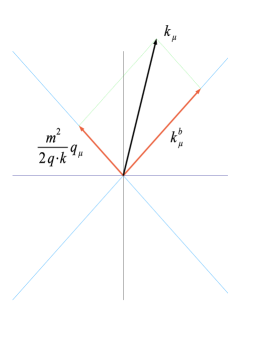
Figure 1: The decomposition of an arbitrary massive vector in 4d on two light-cone vectors [29]

If we have two massive vectors to decompose we can use the formulas

$$k_{1}=k_{1}^{\flat}+{m_{1}^{2}\over s_{12}^{\flat}}k_{2}^{\flat}\ ,\qquad k_{2}=k_{2}^{\flat}+{m_{2}^{2}\over s_{12}^{\flat}}k_{1}^{\flat}\ ,$$ (3)

where we define

$$s_{ij}^{\flat}=2k_{1}^{\flat}\cdot k_{2}^{\flat}=\mathinner{\langle{12}\rangle}[12]$$ (4)

We can define the polarization tensors for a given massive state (gauge boson) as follows [29, 27]

$$e^{+}_{\alpha\dot{\alpha}}=\sqrt{2}\ {k^{\flat}_{\alpha}q_{\dot{\alpha}}\over[qk^{\flat}]}\ ,\quad e^{-}_{\alpha\dot{\alpha}}=\sqrt{2}\ {q_{\alpha}k^{\flat}_{\dot{\alpha}}\over\mathinner{\langle{qk^{\flat}}\rangle}}\ ,\quad e^{0}_{\alpha\dot{\alpha}}={s_{\alpha\dot{\alpha}}\over m}$$ (5)

where $s^{\mu}$ the space-like spin polarization axis

$$s^{\mu}=k^{\mu}-{m^{2}\over k\cdot q}q^{\mu}$$ (6)

It is easy to show that the polarization tensors above satisfy the normalization condition

$$e^{i}_{\mu}e^{j,\mu}={1\over 2}e^{i,\alpha\dot{\alpha}}e^{i}_{\alpha\dot{\alpha}}=\delta_{ij}\ ,\quad i,j=\pm,0$$ (7)

and moreover satisfy the standard completeness relation for massive spin one polarization vectors [28].

We use a standard notation for spinor variables as given in appendix A. Polarization vectors for higher spins states can be written by simple products of the above although to define irreducible representations of the Lorentz $SO(1,3)$ group one should impose the appropriate symmetries dictated by the given Young Tableaux of the representation and of course transversality and tracelessness. Transversality of the polarization tensors (5) to the momentum vector of (1) is automatic. See [27] for an explicit example for the massive spin 2 (level 2 state of the bosonic string).

3 BCFW deformation for a 4-point scattering: General setup

We want to study the $2\to 2$ scattering for open string tachyons in bosonic string theory. We actually choose a configuration where the tachyons carry only 4d momenta. In this manner the intermediate states in the 4-point function will carry only 4d momentum. We will deform particles 1 and 2. The deformation we choose is

$$\hat{k}_{1}=k_{1}+nz\qquad\hat{k}_{2}=k_{2}-nz$$

$$k_{i}\cdot n=n\cdot n=0$$ (8)

and $n=\mathinner{|{2}\rangle}\mathinner{[{1}|}$. The masses are all taken to be $m^{2}_{t}=-1/\alpha^{\prime}$. Moreover we choose to decompose the other two momenta, the unshifted ones, as

$$k_{3}=k_{3}^{\flat}+{m_{t}^{2}\over s_{n3}^{\flat}}n\ ,\qquad k_{4}=k_{4}^{\flat}+{m_{t}^{2}\over s_{n4}^{\flat}}n\ ,$$ (9)

From the above, momentum conservation and (3) it is easy to see that

$$n\cdot k_{3}=n\cdot k_{3}^{\flat}\quad n\cdot k_{4}=n\cdot k_{4}^{\flat}$$

$$n\cdot k_{3}^{\flat}=-n\cdot k_{4}^{\flat}$$ (10)

We also define the Mandelstam variables

$$s=(k_{1}+k_{2})^{2}\ ,\quad t=(k_{1}+k_{4})^{2}\ ,\quad u=(k_{1}+k_{3})^{2}$$ (11)

It is very convenient to define the massless equivalents of the Mandelstam variables

$$s^{\flat}=\mathinner{\langle{12}\rangle}[12]\ ,\quad t^{\flat}=\mathinner{\langle{14}\rangle}[14]\ ,\quad u^{\flat}=\mathinner{\langle{13}\rangle}[13]$$

$$\tilde{s}^{\flat}=\mathinner{\langle{34}\rangle}[34]\ ,\quad\tilde{t}^{\flat}=\mathinner{\langle{23}\rangle}[23]\ ,\quad\tilde{u}^{\flat}=\mathinner{\langle{24}\rangle}[24]$$ (12)

Based on the decomposition above and momentum conservation one can show that

$$s^{\flat}=\tilde{s}^{\flat}$$

$$s+t+u=4m^{2}_{t}\ ,\quad s^{\flat}+t^{\flat}+u^{\flat}=-m^{2}_{t}\ ,\quad s^{\flat}+\tilde{t}^{\flat}+\tilde{u}^{\flat}=-m^{2}_{t}$$ (13)

Finally the Mandelstam kinematic variables are given in terms of the massless ones as

$$s=s^{\flat}+{m^{4}_{t}\over s^{\flat}}+2m^{2}_{t}$$

$$t=t^{\flat}+m^{2}_{t}({\tilde{u}^{\flat}\over s^{\flat}}+2)=\tilde{t}^{\flat}+m^{2}_{t}({u^{\flat}\over s^{\flat}}+2)$$

$$u=u^{\flat}+m^{2}_{t}({\tilde{t}^{\flat}\over s^{\flat}}+2)=\tilde{u}^{\flat}+m^{2}_{t}({t^{\flat}\over s^{\flat}}+2)$$ (14)

Momentum conservation is written as follows

$$\hat{k}_{1}+\hat{k}_{2}+k_{3}+k_{4}=\mathinner{|{1}\rangle}\mathinner{[{1}|}+\mathinner{|{2}\rangle}\mathinner{[{2}|}+\mathinner{|{3}\rangle}\mathinner{[{3}|}+\mathinner{|{4}\rangle}\mathinner{[{4}|}+{m^{2}_{t}\over s^{\flat}}(\mathinner{|{1}\rangle}\mathinner{[{1}|}+\mathinner{|{2}\rangle}\mathinner{[{2}|})=0\ ,$$ (15)

where we have used (3). Using the above we can derive the useful identities

$${\mathinner{\langle{23}\rangle}\over\mathinner{\langle{24}\rangle}}=-{[14]\over[13]}$$

$${\mathinner{\langle{21}\rangle}\over\mathinner{\langle{24}\rangle}}=-{[34]\over[31]}+{m^{2}_{t}\over{\mathinner{\langle{24}\rangle}[12]}}$$ (16)

which of course in the limit $m^{2}_{t}\to 0$ go to the usual identities for the scattering of four massless states.

Moreover since spinors live in a two dimensional space we can always expand one of them as a linear combination of other two i.e.

$$-{[34]\over[31]}\mathinner{[{1}|}+\mathinner{[{4}|}={[14]\over[13]}\mathinner{[{3}|}$$ (17)

We wish to employ the following BCFW recursion relation for the 4-point function. We need to calculate [30]

$${\cal A}^{(1,2)}_{4}(1,2,3,4)=\sum_{N,h(N)}\frac{{\cal A}_{3}(\hat{1},4,\hat{k}_{N})_{z_{res}}{\cal A}_{3}(-\hat{k}_{N},3,\hat{2})_{z_{res}}}{(\hat{k}_{1}+k_{4})^{2}-m_{N}^{2}}\ +\ (3\leftrightarrow 4)$$ (18)

The sum is over all string states of all levels $N$ and we sum over their spins $h(N)$ with respect to the space-like spin axis defined in (6). In figure 2 we show the two terms which contribute above pictorially [30].

$${\cal A}_{4}^{(1,2)}\>=\>\raisebox{63.44952pt}{\scalebox{0.45}{{\includegraphics*[15pt,753pt][463pt,492pt]{tchannel.eps}}}}\;+\;\raisebox{63.44952pt}{\scalebox{0.45}{{\includegraphics*[15pt,753pt][463pt,492pt]{uchannel.eps}}}}$$

Figure 2: Factorization of a four-particle amplitude into two on-shell three-particle amplitudes [30], where $K_{ij}^{2}=(k_{i}+k_{j})^{2}$.

For the time being we assume an abelian theory so the actual order of the states in the 4- and 3- point function is irrelevant. When we will calculate the non-abelian Veneziano amplitude we will be more careful and define properly the order of states at the various vertices.

From the relations above we derive, for the first term in (18) which we call the t-channel, that the poles on the z-plane are given by the relation

$$z_{res}=-{t-m_{N}^{2}\over 2n\cdot k_{4}}=-{m^{2}_{t}-{m^{2}_{N}\over 2}+k_{4}^{\flat}\cdot k_{1}^{\flat}+{m_{t}^{2}\over s_{12}^{\flat}}k_{4}^{\flat}\cdot k_{2}^{\flat}\over n\cdot k_{4}^{\flat}}$$ (19)

and similar for the other term, which we will call the u-channel, with $4\to 3$ and $t\to u$.

Now in order to implement the BCFW procedure we need to follow two steps. First determine the polarization vectors of the intermediate string state and second to apply this to the given cubic vertex. We will discuss the cubic vertex in the following section since this requires a more extended discussion and some assumptions.

In order to define the polarization vectors (5) we need to compute $\hat{k}_{N}=\hat{k}_{1}(z_{res})+k_{4}$ and decompose it into two light-cone vectors. We choose one of them to be $n$ since this will simplify computations substantially later on. Moreover we assume from now one that all hatted quantities are on the residue $z_{res}$. The final result for the momentum vector is

$$\hat{k}_{N}=\hat{k}_{N}^{\flat}+{m_{N}^{2}\over 2n\cdot k_{4}^{\flat}}n=\mathinner{|{\hat{k}_{N}}\rangle}\mathinner{[{\hat{k}_{N}}|}+{m_{N}^{2}\over\mathinner{\langle{24}\rangle}[14]}\mathinner{|{2}\rangle}\mathinner{[{1}|}$$

$$\mathinner{|{\hat{k}_{N}}\rangle}={[14]\over[13]}\mathinner{|{4}\rangle}+{m^{2}_{t}\over\mathinner{\langle{12}\rangle}[13]}\mathinner{|{2}\rangle}\quad\mathinner{[{\hat{k}_{N}}|}=\mathinner{[{3}|}-{m^{2}_{t}\over\mathinner{\langle{23}\rangle}[12]}\mathinner{[{1}|}$$ (20)

The split of $\hat{k}_{N}^{\flat}$ into the two spinors is ambiguous up to phases $\alpha,\beta$ for $\mathinner{|{\hat{k}_{N}}\rangle},\mathinner{[{\hat{k}_{N}}|}$ respectively with $\alpha\cdot\beta=1$. If the spinor decompositions are done correctly the dependance on these two phases should drop out in the final result. Details of this computation appear in appendix B. Using the relations above we can write the polarization vectors

$$\hat{s}=\hat{k}_{N}^{\flat}-{m_{N}^{2}\over 2n\cdot k_{N}^{\flat}}n\,\quad\hat{e}_{0}={\hat{s}\over m_{N}}$$

$$\hat{e}^{+}=-\sqrt{2}{\mathinner{|{\hat{k}_{N}}\rangle}\mathinner{[{1}|}\over[31]}\quad\hat{e}^{-}=-\sqrt{2}{\mathinner{|{2}\rangle}\mathinner{[{\hat{k}_{N}}|}\over\mathinner{\langle{23}\rangle}}$$ (21)

For completeness we also give the expressions

$$\hat{k}_{1}=k_{1}^{\flat}+{m^{2}_{t}\over s^{\flat}}k_{2}^{\flat}-{t-m^{2}_{N}\over\mathinner{\langle{24}\rangle}[14]}\mathinner{|{2}\rangle}\mathinner{[{1}|}$$

$$\hat{k}_{2}=k_{2}^{\flat}+{m^{2}_{t}\over s^{\flat}}k_{1}^{\flat}+{t-m^{2}_{N}\over\mathinner{\langle{24}\rangle}[14]}\mathinner{|{2}\rangle}\mathinner{[{1}|}$$ (22)

We will also need the products of polarization tensors with momenta. Obviously by definition $\hat{e}^{\pm,0}\cdot\hat{k}_{N}=0$. We can easily derive the following

$$\hat{e}^{+}\cdot\hat{k}_{1}=-\hat{e}^{+}\cdot k_{4}={m^{2}_{t}\over\sqrt{2}}\times{\mathinner{\langle{23}\rangle}\over\mathinner{\langle{12}\rangle}[13]}$$

$$\hat{e}^{-}\cdot\hat{k}_{1}=-\hat{e}^{-}\cdot k_{4}=-{1\over\sqrt{2}}{\mathinner{\langle{12}\rangle}[13]\over\mathinner{\langle{23}\rangle}}$$

$$\hat{e}^{0}\cdot\hat{k}_{1}=-\hat{e}^{0}\cdot k_{4}=m_{N}$$ (23)

We also need the polarization products with the momenta $\hat{k}_{2}$ and $k_{3}$

$$\hat{e}^{+}\cdot\hat{k}_{2}=-\hat{e}^{+}\cdot k_{3}={1\over\sqrt{2}}{\mathinner{\langle{23}\rangle}[12]\over[13]}$$

$$\hat{e}^{-}\cdot\hat{k}_{2}=-\hat{e}^{-}\cdot k_{3}=-{m^{2}_{t}\over\sqrt{2}}{[13]\over\mathinner{\langle{23}\rangle}[12]}$$

$$\hat{e}^{0}\cdot\hat{k}_{2}=-\hat{e}^{0}\cdot k_{3}=-m_{N}$$ (24)

Notice that (3) are not given by a simple exchange of labels between $1\to 2$ and $4\to 3$ in (3).

Using the above one can show the important equations

$$X^{+}=\hat{e}^{-}\cdot(\hat{k}_{1}-k_{4})\times\hat{e}^{+}\cdot(k_{3}-\hat{k}_{2})=2s^{\flat}$$

$$X^{-}=\hat{e}^{+}\cdot(\hat{k}_{1}-k_{4})\times\hat{e}^{-}\cdot(k_{3}-\hat{k}_{2})=2{m^{4}_{t}\over s^{\flat}}$$ (25)

and it is easy to show that $X^{+}+X^{-}=2(s-2m^{2}_{t})$. In the expressions above we have ordered the particles as it is dictated by the cubic vertices of figure 2.

4 Cubic vertices for the BCFW relations

We know from [26] that the coupling of a leading Regge trajectory state of level $N$ to two tachyons is given in momentum space by the formula

$${\cal A}_{0-0-N}(k_{I},k_{J},k_{N})=\left({\cal A}^{+}_{bac}\ tr(\tau^{a}\tau^{b}\tau^{c})+{\cal A}^{-}_{abc}\ tr(\tau^{b}\tau^{a}\tau^{c})\right)$$ (26)

where $\tau^{a}$ are $SU(N)$ matrices in the adjoint and

$${\cal A}^{\pm;abc}(k_{I},k_{J},k_{N})={\cal J}_{N}^{\pm;ab}\cdot\phi_{N}^{c}=(\pm\sqrt{{\alpha^{\prime}\over 2}})^{N}\ T_{I}^{a}\ T_{J}^{b}\ \phi_{N}^{c}\cdot k_{12}^{N}\ .$$ (27)

$T_{I}$ the two tachyon fields, $\phi_{N}$ the level N state of the string, $k_{IJ}=k_{I}-k_{J}$ and ${\cal J}_{N}^{\pm;ab}\sim k_{12}^{N}T_{I}^{a}T_{J}^{b}$ the Noether current built from two tachyons [31, 26]. Notice that in the abelian case where the Chan-Paton matrices become unit only even spin particles couple to the two tachyon current. See also the discussion in [30].

This is a covariant coupling and applies to a leading Regge trajectory state of string theory which is traceless and transverse. We would like to infer the couplings of the subleading Regge trajectories. This in principle is a rather complicated task which would require full control of perturbative string theory. Instead of constructing the vertex explicitly we can make an educated guess. We conjecture the following cubic coupling in string light-cone

$${\cal A}_{0-0-N}(k_{I},k_{J},k_{N})=\left({\cal A}^{+}_{abc}(k_{I},k_{J},k_{N})\ tr(\tau^{a}\tau^{b}\tau^{c})+{\cal A}^{-}_{bac}(k_{I},k_{J},k_{N})\ tr(\tau^{b}\tau^{a}\tau^{c})\right)$$ (28)

$${\cal A}^{\pm;abc} (k_{I},k_{J},k_{N};H,h^{+},h^{-})=$$ (29)

$$=(O_{abc})^{H}(\pm 1)^{N}(\sqrt{{\alpha^{\prime}\over 2}})^{H}\ T^{a}_{I}\ T^{b}_{J}\ {(e^{+}\cdot k_{IJ})^{h^{+}}\ (e^{-}\cdot k_{IJ})^{h^{-}}\over\big{(}\prod_{n=1}^{\infty}(n^{h^{+}_{n}}h_{n}^{+}!)(n^{h^{+}_{n}}h_{n}^{+}!)\big{)}^{1/2}}$$

where

$$h_{n}=h^{+}_{n}-h^{-}_{n}\ ,\ \ h=\sum_{n}h_{n}\ ,\ \ N_{n}=h^{+}_{n}+h^{-}_{n}$$

$$h^{\pm}=\sum_{n}h^{\pm}_{n}\ ,\ H=\sum_{n}N_{n}\ ,\ \ N=\sum_{n}N_{n}n$$ (30)

and the light-cone states are not constrained to be in any way traceless but are naturally transverse. We define as $H$ the total $e^{\pm}$ number or in other words the highest spin possible for a given state, $h$ the total spin along the given axis $s^{\mu}$ and the subscripts $n$ are to distinguish the origin of each $e^{\pm}$ in terms of the various levels of the string oscillators. The function $O_{abc}$ is defined as follows for all momenta incoming to the cubic vertex.

$$O_{abc}=\left(\begin{array}[]{cc}+&\qquad cyclic\ (a,b,c)\\ -&\qquad otherwise\end{array}\right)$$ (31)

The purpose of this function is to give to the cubic amplitude the right behavior under the exchange of the external states and in particular under the exchange of the two tachyons. Its presence is dictated by the symmetries of the covariant coupling for the leading Regge trajectory as we will explain shortly.

We would like to justify this vertex. The key point is that we claim that this is the coupling in string light cone in the specific kinematic setup of BCFW (3,9, 3) which is nevertheless sufficient for the BCFW procedure we wish to employ. In other words it is quite general in order to allow using Lorentz invariance to recover the full Veneziano amplitude for general kinematics. Lets give our main arguments which actually sketches a possible rigorous proof which we wont present here but leave for future work. A few more details related to a possible light-cone String Field Theory derivation are given in appendix C. The natural string light-cone frame is defined in appendix B.

• The light-cone states and Regge trajectories. Define string oscillators which satisfy commutator relations

  $$[\alpha^{\mu}_{m},\alpha^{\nu}_{n}]=m\eta^{\mu\nu}\delta_{m+n}\ .$$ (32)

  As it is known in string light-cone the on-shell normalized physical states are given solely in terms of the transverse level $n$ oscillators $\alpha^{i}_{-n}$ through the expression

  $$\mathinner{|{N,k}\rangle}=\prod_{i=2}^{D-1}\ \prod_{n=1}^{\infty}{(\alpha^{i}_{-n})^{N_{in}}\over\big{(}n^{N_{in}}N_{in}!\big{)}^{1/2}}\mathinner{|{0;k}\rangle}$$ (33)

  where $N=\sum_{in}N_{in}n$ the total level of the string state. In [26] the $\mathinner{\langle{\phi_{N},\phi_{N}}\rangle}$ is the symmetrized contraction of the space-time indices and the fields are not normalized to unity while the states above are. Taking this into account, we can write the leading Regge trajectory covariant field $\phi_{N}$ using our normalized polarization vectors (7) in four dimensions as

  $$\phi_{N}=\sum_{h^{\pm},h^{0}}^{h^{+}+h^{-}+h^{0}=N}{(\epsilon^{+})^{h^{+}}(\epsilon^{-})^{h^{-}}(\epsilon^{0})^{h^{0}}\over(h^{+}!h^{-}!h^{0}!)^{1\over 2}}\ .$$ (34)

  This is the properly normalized field as in (33) for a state of level $N$ built only from $a^{\pm,0}_{-1}$.

  Moreover the tachyon current is totally symmetric and therefore as noticed in [26] only the symmetric part of the subleading Regge trajectories will couple. This means that the subleading Regge states which couple to the current are built from the symmetrized products of oscillators $a^{\pm,0}_{-n}$ of all levels similar to (33).

• The coupling to the current. For the tree level amplitudes we want to discuss we can confine ourselves consistently to four dimensions. This is due to the fact that since we have 4d external momenta also the Higher Spin (HS) or reggeon state will have momentum on this 4d subspace. Moreover the coupling above dictates that only polarizations vectors of the reggeon state on this 4d subspace couple to the current built form the two tachyon fields. In other words we do not have traces of the reggeon state coupling to the current. In principle one could have traces of the polarization tensor of the reggeon state in the coupling (29) which effectively would alter the normalization coefficients. The dependance of the coupling in terms of $N,H,h^{+},h^{-}$ would be different and not the one dictated by the assumption that all indices of a given light-cone state couple to the tachyon current. The reasoning behind the aforementioned assumption lies into an appropriate choice string light-cone frame.

  For the purposes of discussing the light-cone setup, lets call the light-cone frame momenta $k_{I}^{(\pm)}$ and the normal components $k_{I}^{i}$. We use parentheses for $(\pm)$ in order to avoid confusion with the $e^{\pm}$ notation above, since this refers to the normal coordinates $i=1,2$. As discussed in [32] in light-cone computations one cannot set all $k^{(+)}_{I}=0$ therefore the vertex operators $e^{ik\cdot X}$ depend on the $X^{(-)}$ component in general. The $X^{(-)}$ in light-cone quantization has an expansion which is quadratic in the oscillators $a^{i}_{-n}$ and therefore if we compute correlators with the states in (33) it results into traces. Also in the operator language there are ”chronic ordering” problems, as explained in chapter 7 of [32], with the definition of the $e^{ik^{(+)}X^{(-)}}$ operators, since $X^{(-)}\sim X^{i}X^{i}$. So usually one has to use the method of light-cone string field theory, see in example chapter 11 of [32]. Nevertheless for few external states it poses no problem to set at least some of the $k^{(+)}_{I}$ momenta equal to zero while preserving the mass-shell conditions $(k_{I}^{i})^{2}=-m_{N}^{2}$. The later assumes complex values for some $k^{i}_{I}$ but in any case we are interested for the 3-point amplitude for complex momenta. We will see in the next section that indeed the BCFW procedure for the Veneziano amplitude can be employed consistently for CM energy $s_{12}<0$ which implies complex momenta for $k_{1,2}$. In appendix B we show that the massive momentum decomposition and BCFW deformation we have employed in this setup leads to a natural string light-cone frame. In this frame one of the tachyon external states of the 3-point function has $\hat{k}^{(+)}_{1}=0$. Moreover since we have only one higher level state (reggeon), polarizations can be chosen arbitrarily enough for our purposes to satisfy transversality in this light-cone frame . The vectors $\hat{e}^{\pm}$ span the transverse space to the string light-cone. With this setup it is fairly easy to see that the coupling of the states (33) to the two tachyons should be proportional to $e^{i}\cdot k_{IJ}$ as in (29) and no traces of the polarizations should appear . We call the transverse coordinates $i=\pm$ from now on.

  Notice that in the above we are referring to the 3-point function we need for the BCFW and not the 4-point we wish to construct. Obviously we assume that with a Lorentz boost we can take the final BCFW constructed 4-point function to an arbitrary frame with unrestricted kinematics. We also do not claim that the momenta of all the n-external states can be put in the light-cone frame with $k^{(+)}_{I}=0,\ I=1,\dots n$. Of course our argument relies on Lorentz invariance of the theory and the assumption of enough generality to allow for the coupling in (29) to reproduce, via the BCFW procedure, the Veneziano amplitude. We give a more explicit discussion on the construction of the vertex based on light-cone String Field Theory in appendix C.

• The phase factor $O_{abc}$. We come now to the $O_{abc}$ function which has an important role. First we will present a formal argument based on cocycles for vertex operators in string theory and then an argument based on the Lorentz properties of the theory.

  A formal argument is based on the following. In the operator formalism computing a correlator one needs to be careful when commuting the positions of two vertex operators. The vertex operators of two tachyons pick-up co-cycle factors

  $$e^{ik_{1}\cdot X(x_{1})}e^{ik_{2}\cdot X(x_{2})}\sim e^{i\pi 2\alpha^{\prime}k_{1}\cdot k_{2}\epsilon(x_{1}-x_{2})}e^{ik_{2}\cdot X(x_{2})}e^{ik_{1}\cdot X(x_{1})}$$ (35)

  where $\epsilon(x_{1}-x_{2})=\pm 1$ for $x_{1}-x_{2}$ greater or less than zero respectively. Using momentum conservation and mass-shell conditions it is straightforward to derive that in a path integral with a state of level N and the two tachyons we have

  $$2\alpha^{\prime}k_{1}\cdot k_{2}=N+1\ .$$ (36)

  Finally for a 3-point function all the operators have a Conformal Killing Ghost $c(x_{I})$ which needs to be commuted as well. Since these are anticommuting fields they contribute and extra minus sign. Therefore taking into account this and (36) in (35) we derive the final phase $(-1)^{N}$ under the exchange of the two tachyons as expected. It depends on the level of the massive string state and not on the actual form of the vertex operator in terms of the oscillators.

  We can actually see the presence of this factor in a more intuitive manner through Lorentz invariance. For the abelian case we know that only even spin couplings exist. The expression in (29) has the right property when inserted in (28). The $(-1)^{N}$ relative factor between ${\cal A}_{\pm;abc}(I,J,N)$ shows that only even spin states contribute which is at least correct for the leading Regge. In a covariant coupling, once it is cast in terms of irreducible representations of the massive little group, the remaining spin multiplets of a given string level would have explicitly this property. Since we are working in a light-cone frame some of this info is not so obvious.

  Take for example the spin 2 massive state. In light-cone the possible states which can couple are composed of $a^{i}_{-1}a^{j}_{-1}$ and $a^{i}_{-2}$ . The first state gives the spin $+2,-2,0$ components of the massive spin 2 multiplet. We always refer to the spin component along the axis of motion. The second state should give the spin $+1,-1$ states. If the coupling for this state is of the form in (29) without the function $O_{abc}$ this would lead into a problem. An exchange of the two tachyons $I\leftrightarrow J$ would give a minus the expression itself and this would mean that it should vanish ((see also [30])). This is obviously unacceptable since this state needs to couple to the tachyon current due to Lorentz invariance of the theory. It is needed to complete the massive spin 2 multiplet. The function $O_{abc}$ takes care of this matter.

  An easy way to see why it should be there is to consider how this state emerges covariantly. The $a^{i}_{2}$ mode is the one of the modes eaten via the Stuckelberg mechanism to give a mass to the spin 2 multiplet. It corresponds to the mode $a^{i}_{-1}a^{0}_{-1}$. Obviously this state is an even rank tensor and gives no problem coupling to the tachyon current under the exchange of tachyon states. One might wonder whether it is possible that one of the subleading Regge trajectory states will couple only partially. That is to couple only those states needed to complete the multiplets coming from the higher spin states but leave the rest out. The entangled way of Stuckelberg mechanism for mass generation of the states and the high symmetry of the coupling does not seem to leave any space for such a scenario. Of course only a direct computation of the cubic coupling would eliminate any doubt about it.

  In the case with Chan-Paton factors we get the usual story of (anti)commutator of Chan-Paton matrices for (even)odd level states.

• Connection to the covariant formulation. Assume we wanted to work in covariant formulation. How would the 3-point amplitude compare to the one computed with the light-cone vertex? Obviously they should have the same physical context modulo the explicit appearance of massive little group representations of $SO(3)$ for the covariant method. We have demonstrated that $\hat{e}^{0}\cdot k_{i}\sim m_{N}=\sqrt{{N-1\over\alpha^{\prime}}}$. So in our BCFW relations, contractions of the zero component polarization tensor give only spin and $\alpha^{\prime}$ dependent terms. Therefore a state $~{}(e^{0})^{h^{0}}(e^{+})^{h^{+}}(e^{-})^{h^{-}}$ will give effectively a BCFW cubic function: $c_{N}({1\over\alpha^{\prime}})^{h_{0}/2}(e^{+})^{h^{+}}(e^{-})^{h^{-}}$, where $c_{N}$ a coefficient dependent on the level of the state and its partitioning in the three polarizations. Therefore in building the leading Regge trajectory coupling for the various modes we will get indeed a coefficient $(\sqrt{{\alpha^{\prime}\over 2}})^{N-h^{0}}=(\sqrt{{\alpha^{\prime}\over 2}})^{H}$, since $N=H+h^{0}$. This is consistent with dimensional analysis of course. The same holds for subleading Regge trajectories as well. The key point is the normalization $c_{N}$ which we claim to be the one of the light-cone states of string theory.

  A direct contact with the covariant formulation would efficiently proceed through the use of DDF [34] states in the OSFT [35] which can be shown to be equivalent with the SFT in light-cone gauge [36].

• Completeness and Orthonormality. We should emphasize that application of the BCFW does not require to decompose the intermediate state in the propagator in terms of irreducible representations of the little group for massive states but rather a complete and orthonormal set of states. The light-cone states comprise such a set although they are not representations of the massive states little group $SO(3)$ in 4d but rather of the massless one $SO(2)$.

After the above discussion we can rewrite in a more manageable form the couplings with CP factors

$${\cal A}_{0-0-N}(k_{I},k_{J},k_{N}) = (O_{abc})^{H}(\sqrt{{\alpha^{\prime}\over 2}})^{H}\ T^{a}_{I}\ T^{b}_{J}$$ (37)

$${(e^{+}\cdot k_{IJ})^{h^{+}}\ (e^{-}\cdot k_{IJ})^{h^{-}}\over\big{(}\prod_{n=1}^{\infty}(n^{h^{+}_{n}}h_{n}^{+}!)(n^{h^{+}_{n}}h_{n}^{+}!)\big{)}^{1/2}}\ tr([\tau^{a},\tau^{b}]_{\pm}\tau^{c})$$

where the $[\cdot\ ,\cdot]_{\pm}$ means (anti)commutator and applies for (even)odd level respectively.

Based on the 3-point amplitude above we will compute the BCFW equation (18). We conclude this section by pointing out that from the ansatz above the main assumptions were the actual normalization of the 3-point function for each light-cone state and the choice of string light-cone frame which sets some of the $k^{+}_{I}=0$. Both the form of the vertex, based on the tachyon current, and the sign factor $O_{abc}$ are pretty much constrained by the symmetries of the vertex and Lorentz invariance of the theory. The power of $\alpha^{\prime}$ is dictated by dimensional analysis. In appendix C we attempt an non-rigorous light-cone SFT derivation which gives nevertheless the full result in (29) even up to the correct normalization. A light-cone or even covariant perturbation theory proof would be highly desirable.

5 3-point functions and combinatorics

The residues of (18) are products of two 3-point functions ${\cal A}_{L}$ and ${\cal A}_{R}$. Each $\hat{e}^{+}$ on ${\cal A}_{L}$ should be accompanied by an $\hat{e}^{-}$ on ${\cal A}_{R}$ and vice-versa since the intermediate state has $+h$ spin for the one amplitude and $-h$ for the other. Moreover the orthogonality of states (33) is based on the orthogonality of the corresponding oscillators upon which they are built. This means that the state which appears on ${\cal A}_{R}$ should be the conjugate of the one in ${\cal A}_{L}$ i.e. $(\hat{e}^{\pm})^{*}=\hat{e}^{\mp}$. So Based on (37) and (3) we see that, each oscillator with a given fixed occupation number $N_{n}$ in a given state gives a contribution to the product of the two 3-point functions as follows

$$({\cal A}_{L}\times{\cal A}_{R})_{N_{n}}=\sum_{h^{+}_{n}}({\alpha^{\prime}\over 2})^{h^{+}_{n}+h^{-}_{n}}{(X^{+})^{h^{+}_{n}}(X^{-})^{h^{-}_{n}}\over h^{+}_{n}!h^{-}_{n}!n^{h^{+}_{n}+h^{-}_{n}}}=$$

$$=\sum_{h^{+}_{n}}{1\over N_{n}!}\ \left(\begin{array}[]{c}N_{n}\\ h^{+}_{n}\end{array}\right){({\alpha^{\prime}\over 2}X^{+})^{h^{+}_{n}}({\alpha^{\prime}\over 2}X^{-})^{h^{-}_{n}}\over n^{N_{n}}}=$$ (40)

$${1\over N_{n}!}{(\alpha(s)+1)^{N_{n}}\over n^{N_{n}}}$$ (41)

where the summation is over all partitionings of $N_{n}$ in $h^{+}_{n}$ with the condition $N_{n}=h^{+}_{n}+h^{-}_{n}$. We also have defined the Regge trajectory

$$\alpha(s)=\alpha^{\prime}s+1$$ (42)

Now we are in position to recover the full contribution of a state of (33) with a given total highest spin $H$

$$({\cal A}_{L}\times{\cal A}_{R})_{H}=\sum_{partN_{n}}\ \prod_{N_{n}}\ {1\over N_{n}!}{(\alpha(s)+1)^{N_{n}}\over n^{N_{n}}}=\sum_{partN_{n}}\ \prod_{N_{n}}{N!\over N_{n}!n^{N_{n}}}\ {(\alpha(s)+1)^{H}\over N!}$$ (43)

where the summation is over all partitionings of the total polarization number (or highest spin $H=\sum_{n}N_{n}$) into the integer numbers $N_{n}$. In the last equation we have defined $N=\sum_{n}N_{n}n$ which is actually the level of the given state.

It turns out that the coefficients of $(\alpha(s)+1)^{H}/N!$ in the expression in (43) are the definition of the Stirling numbers of the first kind

$$S(N,H)=\sum_{partN_{n}}\ \prod_{N_{n}}{N!\over N_{n}!n^{N_{n}}}\ ,\quad N=\sum_{n}N_{n}n\ ,\ \ H=\sum_{n}N_{n}$$ (44)

These count the number of permutations of N elements with H disjoint cycles [33].

To compute the total contribution of a given level N state we need to sum over all the possible oscillator configurations of total number $H$ with upper limit $N$. Actually the Stirling numbers of the first kind generate the Pochhammer symbols and it turns out that

$$({\cal A}_{L}\times{\cal A}_{R})_{N}={1\over N!}\sum_{H=0}^{N}S(N,H)(\alpha(s)+1)^{H}={1\over N!}(\alpha(s)+1)_{N}={\Gamma(\alpha(s)+1+N)\over N!\ \Gamma(\alpha(s)+1)}$$ (45)

In appendix D we show a few examples for the first few levels. Lets consider summing up the result above over all levels in (18). This is not something we do for the abelian case, where only even levels contribute, but certainly it is instructive. The naive result is given by

$${\cal A}^{(1,2)}_{4}(1,2,3,4 t-channel)=\sum_{N=0}^{\infty}\ {1\over N!}{(\alpha(s)+1)_{N}\over\alpha(t)-N}=$$ ;

$$\sum_{N=0}^{\infty}\ {1\over N!}{(\alpha(s)+1)(\alpha(s)+2)\dots(\alpha(s)+N)\over\alpha(t)-N}=-B(-\alpha(s),-\alpha(t))$$

We see that this is one of the terms of the Veneziano amplitude. The series above is defined for the region where $Re(\alpha(s))<0$ and indeed the Pomeron analysis [19, 20, 22] shows that BCFW relations should hold in this region since the asymptotic behavior of the string amplitude under BCFW tachyon deformation is expected to be $z^{1+\alpha^{\prime}s}$. Actually our expansion should be valid in the more constrained domain $|\alpha(s)+1|<1$. We are summing perturbatively over vertices with increasing power of momenta. We can see that this is the case for our result by noticing that $\alpha(s)+1=\alpha^{\prime}k_{1}\cdot k_{2}$. Therefore indeed the actual expansion parameter is $\alpha(s)+1$ and should be in the unit circle on the complex plane for the series to converge.

Then the series can be extended analytically on the whole complex $s$-plane. This in turn demonstrates beautifully the dual nature of the amplitude where the s-channel poles appear after resuming over all the t-channel poles [32]. In the next section we will show explicitly how the results above apply to the Veneziano amplitude for the Abelian and non-Abelian cases.

6 Veneziano amplitude via BCFW

Lets apply (18) to the abelian case using (45) for the contribution of each string level. As we have emphasized before only even level states contribute so we do not expect to derive a beta function immediately as in (5). The two terms in (18) give

$${\cal A}^{(1,2)}_{4}(1,2,3,4)=B^{e}(-\alpha(s);-\alpha(t))+B^{e}(-\alpha(s);-\alpha(u))$$ (47)

where we have defined the following expressions

$$B^{e}(-x;-y)=\sum_{N\in 2\mathbb{N}}\ {1\over N!}{(x+1)_{N}\over y-N}$$

$$B^{o}(-x;-y)=\sum_{N\in 2\mathbb{N}+1}\ {1\over N!}{(x+1)_{N}\over y-N}$$ (48)

The expressions above do not have the appropriate duality properties of the beta functions so the order of their arguments is important. They can be rewritten in terms of hypergeometric functions but there is no obvious way to transform them into beta functions as expected.

Now we will show the expression in (47) is actually proportional to the abelian Veneziano amplitude

$${\cal A}_{4}=-{1\over 2}\left[B(-\alpha(s),-\alpha(t))+B(-\alpha(s),-\alpha(u))+B(-\alpha(t),-\alpha(u))\right]$$ (49)

The first and most important observation is that the two results in (47) and (49) have the same residues in the t- and u-channels. The odd residues of the beta function in the t-channel cancel between $B(-\alpha(s),-\alpha(t))$ and $B(-\alpha(t),-\alpha(u))$ and similar statement holds for the odd u-channel poles. Now it is obvious that the result in (47) should reproduce the $B(-\alpha(t),-\alpha(u))$ term although it is not evident at first sight. We use the exact same reasoning as in [32]) chapter 1 for the beta function written as a series of its poles in one channel in the region where in other channel it has no pole.

In the region of series convergence $Re(\alpha(s))<0$, (49) has no s-channel poles. Moreover the residues of the two expressions (49) and (47) agree. Therefore they can only differ by an entire function in the $t,u$ variables. Since such an entire function which vanishes for large $|\alpha(t)|$ and $|\alpha(u)|$ does not exist then we can conclude that the two expressions are identical. Therefore we just need to show that the Veneziano amplitude (49) vanishes when either $|\alpha(t)|$ or $|\alpha(u)|$ go to infinity. Actually it turns out that both moduli of these variables need to go to infinity at the same time and not just either of them. The reason is momentum conservation

$$\alpha(s)+\alpha(t)+\alpha(u)=-1$$ (50)

In the previous section we pointed out that actually the BCFW procedure we employed is valid only in the more constrained domain $-2<\alpha(s)<1$. Therefore in the large $|\alpha(t)|$ regime we have $\alpha(u)\simeq-\alpha(t)$ and $|\alpha(u)|$ goes so infinity as well. Applying this limit to (49) and using Stirling approximation we get

$${\cal A}_{4}\simeq\Gamma(-\alpha(s))\left((-\alpha(t))^{\alpha(s)}+(-\alpha(u))^{\alpha(s)}\right)+(\alpha(t))^{-{1\over 2}}\ 2^{\alpha(s)-{3\over 2}}$$ (51)

We see that indeed for $Re(\alpha(s))<0$ the amplitude goes to zero as expected due to the constructibility proof using Pomeron operators. We can analytically continue this expression outside the region of convergence of the series and this we way we will recover the full Veneziano amplitude. This concludes the proof of the BCFW construction for the abelian Veneziano amplitude. One can check the constructibility criterion of [30] by deforming the particles 1 and 4. The final result is the same.

Lets summarize the following identities which are derived with the methodology above based on the assumptions of convergence of the series and also momentum conservation (50). They will be useful for the rest of this section.

$$B^{e}(-x;-y)+B^{o}(-x;-y)=-B(-x,-y)$$

$$B^{e}(-\alpha(s);-\alpha(t))+B^{e}(-\alpha(s);-\alpha(u))=$$

$$=-{1\over 2}\left(B(-\alpha(s),-\alpha(t))+B(-\alpha(s),-\alpha(u))+B(-\alpha(t),-\alpha(u))\right)$$

$$B^{o}(-\alpha(s);-\alpha(t))+B^{o}(-\alpha(s);-\alpha(u))=$$

$$=-{1\over 2}\left(B(-\alpha(s),-\alpha(t))+B(-\alpha(s),-\alpha(u))-B(-\alpha(t),-\alpha(u))\right)$$ (52)

Now we will proceed with the Non-abelian case. Using the vertices in (37) it is straightforward to derive from the two terms in (18) the following

$${\cal A}_{4}^{(1,2)}={\cal A}^{(1,2)}_{t}+{\cal A}^{(1,2)}_{u}=$$ (53)

$$=tr\left(\{t^{1},t^{4}\}\{t^{3},t^{2}\}\right)B^{e}(-\alpha(s);-\alpha(t))+tr\left([t^{1},t^{4}][t^{3},t^{2}]\right)(B^{o}(-\alpha(s);-\alpha(t)))+$$

$$+tr\left(\{t^{1},t^{3}\}\{t^{4},t^{2}\}\right)B^{e}(-\alpha(s);-\alpha(u))+tr\left([t^{1},t^{3}][t^{4},t^{2}]\right)(B^{o}(-\alpha(s);-\alpha(u)))$$

where we have used the standard notation for (anti)commutators. Expanding in color ordered factors we get

$${\cal A}_{4}^{(1,2)}=tr\left(t^{1}t^{4}t^{3}t^{2}+t^{1}t^{2}t^{3}t^{4}\right)\left(B^{e}(-\alpha(s);-\alpha(t))+B^{o}(-\alpha(s);-\alpha(t))\right)+$$

$$+tr\left(t^{1}t^{3}t^{4}t^{2}+t^{1}t^{2}t^{4}t^{3}\right)\left(B^{e}(-\alpha(s);-\alpha(u))+B^{o}(-\alpha(s);-\alpha(u))\right)+$$

$$+tr\left(t^{1}t^{4}t^{2}t^{3}+t^{1}t^{3}t^{2}t^{4}\right)(B^{e}(-\alpha(s);-\alpha(t))+B^{e}(-\alpha(s);-\alpha(u))-$$

$$-B^{o}(-\alpha(s);-\alpha(t))-B^{o}(-\alpha(s);-\alpha(u)))$$ (54)

and using the identities in (6) we easily derive the Veneziano amplitude for the non abelian case

$${\cal A}_{4}=-tr\left(t^{1}t^{4}t^{3}t^{2}+t^{1}t^{2}t^{3}t^{4}\right)B(-\alpha(s);-\alpha(t))-$$

$$-tr\left(t^{1}t^{3}t^{4}t^{2}+t^{1}t^{2}t^{4}t^{3}\right)B(-\alpha(s);-\alpha(u))-$$

$$-tr\left(t^{1}t^{4}t^{2}t^{3}+t^{1}t^{3}t^{2}t^{4}\right)B(-\alpha(t);-\alpha(u))$$ (55)

A deformation of the particles 1 and 4 gives identical result as required by the consistency condition of [30].

7 Conclusions and Outlook

We have proposed an explicit construction of the Veneziano amplitude based on the BCFW procedure. We first applied the methodology of spinor helicity formulation for massive states as i.e. [20]. Then we proceeded with a conjecture on the 3-point function of an arbitrary massive state of string theory with two tachyons in a kinematic frame we consider general enough for our purposes. We gave some arguments which support its form but a lack of rigorous proof is definitely an unsatisfying state of affairs. We applied the conjectured 3-point function to the BCFW recursion formulas for the construction of the 4-point function for four external tachyons. After some interesting combinatorics we managed to show how the celebrated Beta functions of the Veneziano amplitude arise. We sum up an infinite number of massive string exchanges in the channels which become deformed under the BCFW deformation. The dual behavior of the Veneziano amplitude emerges from an analytic continuation of the formal series in the kinematic region where poles in the dual channels appear.

Thinking inversely our cubic couplings can be taken as derived via the BCFW method. The residues of the BCFW deformation of the 4-point function determine the product (43) which can be reproduced as we have shown by the cubic couplings (37). So our proposed 3-point function can be taken as derived rather than conjectured although the inverse procedure we claim above does non necessarily lead to unique 3-point functions (see for example [19] where the BCFW deformation of the five tachyon amplitude can be written as a recursion relation in terms of only tachyon sub-amplitudes).

We would like to make a few comments and clarifications regarding the BCFW procedure itself for string amplitudes. One should not confuse the BCFW recursion relations with the usual string world-sheet factorizations when a kinematic invariant approaches a physical pole . Definitely due to unitarity the string amplitude factorizes on the poles to lower on-shell string amplitudes. But these amplitudes are defined on the special kinematics of the external states and do not constitute a recursive construction of the string amplitude away from these special points. In the BCFW relations the lower point amplitudes are computed on complex momenta which differ from the momenta of the actual physical residues.

Moreover the BCFW method reconstructs the string amplitude using the residues of only a subset of all the possible channels. These are the Reggerized channels. In the Pomeron language used in [19, 20, 22] these channels correspond to the shifted kinematic variables. The large Regge behavior is dictated by the unshifted kinematic variable i.e. ${\cal A}\sim(\hat{t})^{\alpha^{\prime}s}$. Keeping the unshifted kinematic variables in the region where the Regge channel becomes damped for large shifts, we are guaranteed the absence of a residue at infinity. The un-reggerized channels are reconstructed by analytic continuation of the unshifted momenta outside the aforementioned region. The BCFW reconstruction of the string amplitude looks like an expansion in terms Feynman diagrams for tree level field theory exchanges. In the region where the BCFW method is applicable we can think of the world-sheet as thinning out as we approach the poles of the deformed amplitude. The residues of the poles in the Reggerized channel reconstruct in a way the world-sheet locally. Then moving outside this region we recover the full world-sheet. It is in complex momenta for the exchanged particle that this description is possible without restricting the momenta of the external states to special values.

Another thing to point out is that, just as in gauge theory applications of BCFW, individual terms of the recursion relations might exhibit spurious poles (see i.e. [8]) which do not correspond to physical poles. These should cancel in the final expression and indeed this is a strong consistency check for the validity of the BCFW method.

There are several directions one should follow. The foremost important is a rigorous derivation of the 3-point amplitude proposed in (37). Definitely if such a result cannot be reconstructed then it will be quite remarkable that the conjectured 3-point vertex reproduces the Veneziano amplitude. It is not clear what would be the physical meaning of such a result.

The next step would be to use the general 3-point vertex for external string states of arbitrary level (reggeons) [39] with appropriate choices of kinematic regions to see if we can reproduce higher point tachyon amplitudes. Even for recursion relations for the five tachyon amplitude one would need at least the one tachyon with two reggeons amplitude. This way one could compute the 4-point function of three tachyons and on reggeon which is needed for applying the BCFW method in this case. Constructing the five tachyon amplitude is highly non-trivial task which will uncover any potential problems in applying the BCFW method for string amplitudes.

Obviously the most interesting cases lie in the context of superstring theory. Tree level gluon amplitudes do not depend on the compactification details of the internal coordinates in string theory [16]. So it is very interesting phenomenologically to construct recursion relations which allow us to compute the leading string corrections to the n-gluon amplitudes. Therefore an obvious generalization of the present work is its extension to superstring theory. A good starting point would be the supersymmetric three reggeon vertex of [37].

Beyond the obvious applications for string amplitude computations one of the motivations for the present work is to try to extend to string theory many of the present developments, like i.e. the Grassmannian [8], integrability [38] for ${\cal N}=4$ SYM, BCFW relations for loop amplitudes [10, 11] e.t.c. In this case we might be able to learn more about the symmetries of the theory or its non-perturbative properties.

Appendix A: Notation and a Basis of Vectors

We use the definitions

$$\mathinner{\langle{\lambda\lambda^{\prime}}\rangle}=\epsilon^{\alpha\beta}\lambda_{\alpha}\lambda_{\beta}^{\prime}\ ,\quad[\tilde{\lambda}\tilde{\lambda}^{\prime}]=\epsilon^{\alpha\beta}\tilde{\lambda}_{\dot{\alpha}}\tilde{\lambda}_{\dot{\beta}}^{\prime}$$ (A.1)

and for light-cone vectors we use

$$k^{\mu}=\lambda^{\alpha}\sigma^{\mu}_{\alpha\dot{\alpha}}\tilde{\lambda}^{\dot{\alpha}}\ ,\quad 2p\cdot q=\mathinner{\langle{\lambda^{p}\lambda^{q}}\rangle}[\tilde{\lambda}^{p}\tilde{\lambda}^{q}]$$ (A.2)

The metric we use is $(+,-,-,-)$ and $\sigma^{\mu}=(1,\sigma^{i})$. The following identities and definitions are used in many cases in the spinor helicity formalism

$$(\bar{\sigma}^{\mu})^{\alpha\dot{\alpha}}=-\epsilon^{\alpha\beta}\epsilon^{\dot{\alpha}\dot{\beta}}(\sigma^{\mu})_{\beta\dot{\beta}},\quad\epsilon^{12}=\epsilon_{12}=1$$

$$(\bar{\sigma}_{\mu})^{\alpha\dot{\alpha}}(\sigma^{\mu})^{\beta\dot{\beta}}=2\delta^{\beta}_{\alpha}\delta^{\dot{\alpha}}_{\dot{\beta}}\ .$$ (A.3)

With the definitions above we can write an arbitrary 4-vector $k^{\mu}$ in matrix notation

$$k^{\mu}=\left(\begin{array}[]{cc}k^{0}+k^{3}&k^{1}+ik^{2}\\ k^{1}-ik^{2}&k^{0}-k^{3}\end{array}\right)$$ (A.4)

where $\det(k^{\mu})=m^{2}$. Polarization for integer spin-$s$ massless particles are given in terms of the polarizations for massless spin 1 particles

$$e^{+}_{\alpha_{1}\dot{\alpha}_{1},\dots\alpha_{s}\dot{\alpha}_{s}}=\prod_{i=1}^{s}e^{+}_{\alpha_{i}\dot{\alpha}_{i}}\ ,\quad e^{-}_{\alpha_{1}\dot{\alpha}_{1},\dots\alpha_{s}\dot{\alpha}_{s}}=\prod_{i=1}^{s}e^{-}_{\alpha_{i}\dot{\alpha}_{i}}$$ (A.5)

where the spin 1 polarization vectors are given by

$$e^{+}_{\alpha\dot{\alpha}}=\sqrt{2}\ {\lambda_{\alpha}\tilde{\mu}_{\dot{\alpha}}\over[\tilde{\mu}\lambda]}\ ,\quad e^{-}_{\alpha\dot{\alpha}}=\sqrt{2}\ {\mu_{\alpha}\tilde{\lambda}_{\dot{\alpha}}\over\mathinner{\langle{\mu\tilde{\lambda}}\rangle}}$$ (A.6)

and $\mu_{\alpha}$, $\tilde{\mu}_{\dot{\alpha}}$ arbitrary reference spinors. A change in the reference spinors corresponds to a gauge transformation of the polarization tensors for the massless states and a given amplitude must be invariant under such a transformation.

Appendix B: Polarization calculation

The first relation we will prove is (3). Write the momentum of the intermediate state using

$$\hat{k}_{N}=k_{1}^{\flat}+k_{4}^{\flat}+{m^{2}_{t}\over s^{\flat}}k_{2}^{\flat}+{m^{2}_{t}\over 2k_{4}^{\flat}\cdot n}n-{m^{2}_{t}-m^{2}_{N}/2+k_{4}^{\flat}\cdot k_{1}^{\flat}+{m^{2}_{t}\over s^{\flat}}k_{4}^{\flat}\cdot k_{2}^{\flat}\over n\cdot k_{4}^{\flat}}n$$ (B.1)

We can show the following identities:

$$k_{1}^{\flat}+k_{4}^{\flat}-n{k_{4}^{\flat}\cdot k_{1}^{\flat}\over k_{4}^{\flat}\cdot n}={\mathinner{\langle{21}\rangle}\over\mathinner{\langle{24}\rangle}}\mathinner{|{4}\rangle}\mathinner{[{1}|}+\mathinner{|{4}\rangle}\mathinner{[{4}|}$$ (B.2)

using (3) and linear dependance of the spinors $\mathinner{[{1}|},\mathinner{[{3}|},\mathinner{[{4}|}$.

$${m^{2}_{t}\over s^{\flat}}(k_{2}^{\flat}-{k_{4}^{\flat}\cdot k_{2}^{\flat}\over k_{4}^{\flat}\cdot n}n)={m^{2}_{t}\over\mathinner{\langle{12}\rangle}[14]}\mathinner{|{2}\rangle}\mathinner{[{4}|}$$ (B.3)

using linear dependance of $\mathinner{[{1}|},\mathinner{[{2}|},\mathinner{[{4}|}$.

$${m^{2}_{t}\over\mathinner{\langle{12}\rangle}[14]}\mathinner{|{2}\rangle}\mathinner{[{4}|}-{m^{2}_{t}\over\mathinner{\langle{24}\rangle}[14]}\mathinner{|{2}\rangle}\mathinner{[{1}|}={m^{2}_{t}\over\mathinner{\langle{12}\rangle}[13]}\mathinner{|{2}\rangle}\mathinner{[{3}|}+{m^{4}_{t}\over s^{\flat}\mathinner{\langle{24}\rangle}[14]}\mathinner{|{2}\rangle}\mathinner{[{1}|}$$ (B.4)

using the second of (3) and linear dependance of $\mathinner{[{1}|},\mathinner{[{3}|},\mathinner{[{4}|}$. All of the above lead to (3).

From the polarization contractions only the $\hat{e}^{0}\cdot\hat{k}_{1}=-\hat{e}^{0}\cdot k_{4}$ is a tedious one. The other ones come easily with application of (3). We show some intermediate steps form the $\hat{e}^{0}$ polarization manipulations

$$\hat{e}^{0}\cdot\hat{k}_{1}={\hat{k}_{N}^{\flat}\cdot\hat{k}_{1}\over m_{N}}=$$

$$={-1\over 2m_{N}}\{{[14]\over[13]}(\mathinner{\langle{41}\rangle}[13]+m^{2}_{t}{\mathinner{\langle{42}\rangle}[23]\over s^{\flat}})+(t-m_{N}^{2})+{m^{4}_{t}\over s^{\flat}}-m^{2}_{t}\}=$$

$$={-1\over 2m_{N}}\{-t^{\flat}+m^{2}_{t}({\tilde{t}^{\flat}\over s^{\flat}}-1)+{m^{4}_{t}\over s^{\flat}}+(t-m^{2}_{N})\}=$$

$$={m_{N}\over 2}$$ (B.5)

One can easily guess that $\hat{e}^{0}\cdot\hat{k}_{1}=-\hat{e}^{0}\cdot k_{4}$ since $\hat{e}^{0}\cdot\hat{k}_{N}=0$ but as a useful cross-check of our calculations we can explicitly show that

$$\hat{e}^{0}\cdot k_{4}=(\hat{k}_{N}^{\flat}-{m^{2}_{N}\over 2n\cdot\hat{k}_{N}^{\flat}}n)\cdot{k_{4}\over m_{N}}=$$

$$=-{1\over 2m_{N}}\{(-m^{2}_{t}+m^{2}_{t}{\mathinner{\langle{24}\rangle}[43]\over\mathinner{\langle{12}\rangle}[13]}-{m^{4}_{t}\over s^{\flat}})+m^{2}_{N}\}=$$

$$=-{m_{N}\over 2}$$ (B.6)

Now we proceed in defining a convenient ”light-cone” basis of vectors which will turn useful in discussing the 3-point amplitude needed for the BCFW relations. We use the light-cone vectors used to define $\hat{k}_{N}$ in order to write down a basis as in [29]

$$v_{1}={\mathinner{|{\hat{k}_{N}}\rangle}\mathinner{[{\hat{k}_{N}}|}\over m_{N}}\ ,\quad v_{3}={\mathinner{|{2}\rangle}\mathinner{[{\hat{k}_{N}}|}\over\mathinner{\langle{2\hat{k}_{N}}\rangle}}$$

$$v_{2}=m_{N}{\mathinner{|{2}\rangle}\mathinner{[{1}|}\over\mathinner{\langle{2\hat{k}_{N}}\rangle}[1\hat{k}_{N}]}\ ,\quad v_{4}={\mathinner{|{\hat{k}_{N}}\rangle}\mathinner{[{1}|}\over[1\hat{k}_{N}]}$$ (B.7)

The elements $v_{1}$ and $v_{2}$ are the light-cone vectors used to define the momentum vector $\hat{k}_{N}$ and the other two vectors $v_{4}$ and $v_{3}$ are proportional to the polarization vectors $\hat{e}^{+}$ and $\hat{e}^{-}$ respectively. There exists a frame where the basis vectors in (Appendix B: Polarization calculation) take the form

$$\begin{array}[]{cccc}v^{1}_{\mu}\sim\left(\begin{array}[]{c}1\\ 0\\ 0\\ 1\end{array}\right)&v^{2}_{\mu}\sim\left(\begin{array}[]{c}1\\ 0\\ 0\\ -1\end{array}\right)&v^{3}_{\mu}\sim\left(\begin{array}[]{c}0\\ 1\\ i\\ 0\end{array}\right)&v^{4}_{\mu}\sim\left(\begin{array}[]{c}0\\ 1\\ -i\\ 0\end{array}\right)\end{array}$$ (B.8)

with

$$v^{1;\mu}v^{2}_{\mu}+v^{3;\mu}v^{4}_{\mu}=0.$$ (B.9)

As explained in [29] an arbitrary 4-vector can be expanded in the following manner

$$k_{\mu}=c_{1}v_{1}+c_{2}v_{2}+c_{3}v_{3}+c_{4}v_{4}=$$

$$\equiv k_{\mu}^{\flat}+{k^{2}\over 2v_{3}\cdot k}v_{3}$$ (B.10)

where the basis vector $v_{3}$ was chosen arbitrarily to define the second light-cone vector, in addition to $k^{\flat}_{\mu}$, needed for the decomposition of the vector $k_{\mu}$. We can determine the coefficients $c_{i}$ as follows

$$c_{1}=-m_{N}{\mathinner{\langle{2}|}k\mathinner{|{1}]}\over 2\hat{k}^{\flat}_{N}\cdot n}\ ,\quad c_{2}=-{\mathinner{\langle{\hat{k}_{N}}|}k\mathinner{|{\hat{k}_{N}}]}\over m_{N}}$$

$$c_{3}=-{\mathinner{\langle{\hat{k}_{N}}|}k\mathinner{|{1}]}\over[1\hat{k}_{N}]}\ ,\quad c_{4}=-{\mathinner{\langle{2}|}k\mathinner{|{\hat{k}_{N}}]}\over\mathinner{\langle{2\hat{k}_{N}}\rangle}}$$ (B.11)

We can indeed check that for an arbitrary vector with decomposition

$$k^{\mu}=a^{\mu}+{m^{2}\over\mathinner{\langle{ab}\rangle}[ab]}b^{\mu}$$

the determinant of the matrix

$$\left(\begin{array}[]{cc}c_{1}&c_{4}\\ c_{3}&c_{2}\end{array}\right)$$

is equal to $m^{2}$ as it is required by (A.4) using (B.9). To prove the statement above we have to use the Schouten identity

$$\mathinner{\langle{xy}\rangle}\mathinner{\langle{wz}\rangle}+\mathinner{\langle{xz}\rangle}\mathinner{\langle{yw}\rangle}+\mathinner{\langle{xw}\rangle}\mathinner{\langle{zy}\rangle}=0\ .$$ (B.12)

Then it is easy to see that in this frame the momentum vectors of the three particles $\hat{k}_{1},\ k_{4}$ and $\hat{k}_{N}$ are written in matrix notation as

$$\hat{k}_{N}^{\mu}=\left(\begin{array}[]{cc}m_{N}&0\\ 0&m_{N}\end{array}\right)$$ (B.15)

$$k_{4}^{\mu}=\left(\begin{array}[]{cc}m_{N}&{\mathinner{\langle{12}\rangle}[13]\over\mathinner{\langle{23}\rangle}}\\ -{m^{2}_{T}\mathinner{\langle{23}\rangle}\over\mathinner{\langle{12}\rangle}[13]^{3}}&0\end{array}\right)$$ (B.18)

$$\hat{k}_{1}^{\mu}=\left(\begin{array}[]{cc}0&-{\mathinner{\langle{12}\rangle}[13]\over\mathinner{\langle{23}\rangle}}\\ {m^{2}_{T}\mathinner{\langle{23}\rangle}\over\mathinner{\langle{12}\rangle}[13]}&m_{N}\end{array}\right)$$ (B.21)

where we have used equations (Appendix B: Polarization calculation), (Appendix B: Polarization calculation) and (3, 9) to determine the diagonal components of $\hat{k}_{1}$ and $k_{4}$. We also used the expressions in (3) to calculate the off-diagonal components. It is obvious by simple inspection of (A.4) that $\hat{k}_{1}^{(+)}=0$ and $k_{4}^{(-)}=0$ with respect to the light-cone frame defined by the vectors $\hat{k}^{\flat}$ and $n$. So the decomposition of the external momenta in terms of $n$ being one of the two light-cone vectors results in the natural basis (Appendix B: Polarization calculation) which in turn dictates that one of the two external momenta i.e. $\hat{k}_{1}$ has vanishing $\hat{k}_{1}^{(+)}$ component. This serves in the simplicity of the cubic vertex (29) as it is explained in section 4 and in appendix C.

Appendix C: Light-cone String Field Theory

In order to derive the form of the vertex in (29) one has to rely to SFT in the light-cone gauge. The main formulas for the cubic vertex are given in chapter 11 of [32]

$$\mathinner{|{V_{3}}\rangle}=exp\left(-\tau_{0}\sum_{r}{1\over\alpha_{r}}+\Delta_{B}\right)\mathinner{|{0}\rangle}\delta\left(\sum_{r}p_{r}\right)$$ (C.1)

where

$$\Delta_{B}={1\over 2}\sum_{r,s}\sum_{m,n=1}^{\infty}\bar{N}^{rs}_{mn}\ \alpha_{-m}^{r}\cdot\alpha_{-n}^{s}+\sqrt{2\alpha^{\prime}}\sum_{r}\sum_{m=1}^{\infty}\bar{N}^{r}_{m}\alpha_{-m}^{r}\cdot P+\alpha^{\prime}{\tau_{0}\over\hat{\alpha}}P^{2}$$ (C.2)

and $r=1,2,3$ run over the three Hilbert spaces for the particles of interest. The definitions of the Neumann matrices are

$$\bar{N}^{r}_{m}=N^{r}_{m}e^{m\tau_{0}/\alpha_{r}}\ ,\quad N^{r}_{m}={1\over\alpha_{r}}f_{m}(-{\alpha_{r+1}\over\alpha_{r}})$$

$$N^{rs}_{mn}=-{mn\alpha_{1}\alpha_{2}\alpha_{3}\over n\alpha_{r}+m\alpha_{s}}N^{r}_{m}N^{s}_{n}$$

$$f_{m}(\gamma)={(-1)^{m-1}\over m!}{\Gamma(m-m\gamma)\over\Gamma(1-m\gamma)}$$ (C.3)

The parameters of the vertex are defined as

$$P=\alpha_{1}k_{2}-\alpha_{2}k_{1}\ ,\quad\tau_{0}=\sum_{r=1}^{3}\alpha_{r}\log|\alpha_{r}|\ ,\quad\hat{\alpha}=\alpha_{1}\alpha_{2}\alpha_{3}$$ (C.4)

The string ”lengths” are given by the relation $\alpha_{r}=2k^{(+)}$ and they satisfy due to momentum conservation the relations

$$\sum_{r=1}^{3}{k^{2}_{r}\over\alpha_{r}}=-{P^{2}\over\hat{\alpha}}\ ,\quad\sum_{r}\alpha_{r}=0$$ (C.5)

Moreover the above imply that $P$ is cyclic in the Hilbert indices something which is not obvious in (Appendix C: Light-cone String Field Theory) and that for the $\alpha_{r}$ variables holds a cyclic property with the identification $\alpha_{4}=\alpha_{1}$.

With real momenta it is not a’priori possible to set any of the parameters $\alpha_{r}=0$. This is obvious since this would contradict the on shell condition $2k^{(+)}k^{(+)}-(k^{i})^{2}=m_{N}^{2}$. But with complex momenta we can see that such a choice is possible. We saw in appendix B that the massive momentum decomposition for the BCFW setup leads naturally to a light-cone frame where the momentum of one of the tachyons has $\hat{k}^{(+)}_{1}=0$ .

For our purposes we can put the two tachyons in Hilbert spaces $r=1,2$ and the reggeon state in $r=3$. We can choose $\alpha_{1}=0$. This in terms of our setup in BCFW means that we can choose the string light cone frame as in (Appendix B: Polarization calculation). Since only the state in the third Hilbert space is a reggeon state and the other two are vacuum states (tachyons), we have to consider only the behavior of the Neumann coefficient of the third Hilbert space for this configuration . We can easily see that the following identities hold

$$\alpha_{2}=-\alpha_{3}\ ,\quad P=-\alpha_{2}k_{1}\,\quad\tau_{0}\to 0$$

$$-\tau_{0}\sum_{r}{1\over\alpha_{r}}+\alpha^{\prime}{\tau_{0}\over\hat{\alpha}}P^{2}=\log|\alpha_{1}|\left(1+\alpha^{\prime}k_{1}^{2}\right)=0$$

$$N^{3}_{m}={1\over a_{3}}{(-1)^{m-1}\over m}\ ,\quad N^{3}_{mn}=0\ ,\quad\bar{N}^{3}_{m}=N^{3}_{m}$$ (C.6)

where we have used the mass-shell condition for the tachyon $k_{1}^{2}=-{1\over\alpha^{\prime}}$. So we see that the Neumann coefficients which would lead into traces are eliminated in this case. We are left only with

$$\Delta_{B}=\sqrt{2\alpha^{\prime}}\sum_{m=1}^{\infty}\bar{N}^{3}_{m}\alpha_{-m}^{3}\cdot P$$ (C.7)

Acting on a state as in (33) and two tachyons and restricting to 4-dimensions we indeed get the result in (29)up to a phase. To prove this we have to use the oscillator algebra (32) and make the substitution $e^{\pm}\cdot k_{1}={1\over 2}e^{\pm}\cdot(k_{1}-k_{2})$ due to momentum conservation and transversality of the polarization to $k_{3}=k_{1}+k_{2}$ . The $(-1)^{m-1}$ factors give $(-1)^{N}\times(-1)^{H}$. The phase $(-1)^{H}$ is equivalent to our $O_{abc}^{H}$.

We could call the above a proof if it was not for the possibly singular choice of $a_{r}$ we have made. A more precise derivation should follow the result of [39]. Specifically their equation (5.14) includes traces of the reggeon state which are given in the string light-cone by $\sum_{i=1}^{24}e^{i}\cdot e^{i}=24$. Definitely the vertex derived in this work differs from ours. It has as a leading derivative proportional to the vertex (29) but also lower derivative ones since it corresponds to generic configurations with $k^{(+)}_{1}\neq 0$. Nevertheless the statement we wish to make is that the final result of the BCFW construction will be the same. In other words it will agree with the BCFW result using the light-cone vertex in the particular light-cone frame we have used in this paper. To prove this, one could choose a different light-cone frame and repeat the analysis from scratch. This means a different set of light-cone vectors in place of $\hat{k}_{N}\ ,n$ but also different set of polarization vectors $\hat{e}^{\pm}$. This point definitely deserves further study.

Appendix D: A few examples on level contributions

Consider the contribution to (43) of the level 1 state. There is only one oscillator in this case and the light cone state is written as

$$\mathinner{|{1,k}\rangle}=a^{\pm}_{-1}$$ (D.1)

This automatically leads to the contribution to the residue of BCFW from (5) for $N_{n}=1$

$$({\cal A}_{L}\times{\cal A}_{R})_{1}={\alpha(s)+1\over 1!}$$ (D.2)

For this level there is only one contribution and this agrees with the (45) for $N=1$.

Level $N=2$ is the first level where the particular normalization of our state will become important. The light-cone states and their contributions are

$${a^{\pm}_{-2}\over 2\ 1!}\rightarrow{\alpha(s)+1\over 2}$$

$${(a^{\pm}_{-1})^{2}\over 2!}\rightarrow{(\alpha(s)+1)^{2}\over 2}$$ (D.3)

Summing all of the above contributions we can easily derive (45) for $N=2$

$$({\cal A}_{L}\times{\cal A}_{R})_{2}={(\alpha(s)+1)(\alpha(s)+2)\over 2!}$$ (D.4)

The next level is $N=3$. There are three light-cone states and we give their contribution from (5)

$${a^{\pm}_{-3}\over 3\ 1!}\rightarrow{\alpha(s)+1\over 3}$$

$${a^{\pm}_{-2}\ a^{\pm}_{-1}\over 2\ 1!\ 1!}\rightarrow{(\alpha(s)+1)^{2}\over 2}$$

$${(a^{\pm}_{-1})^{3}\over 3!}\rightarrow{(\alpha(s)+1)^{3}\over 6}$$ (D.5)

Summing all of the above contributions we can easily derive (45) for $N=3$

$$({\cal A}_{L}\times{\cal A}_{R})_{3}={(\alpha(s)+1)(\alpha(s)+2)(\alpha(s)+3)\over 3!}$$ (D.6)

Level 4 goes along the same lines.

References

- [1] E. Witten, “Perturbative gauge theory as a string theory in twistor space,” Commun. Math. Phys. 252 (2004) 189 [arXiv:hep-th/0312171].
- [2] F. Cachazo, P. Svrcek and E. Witten, “MHV vertices and tree amplitudes in gauge theory,” JHEP 0409 (2004) 006 [arXiv:hep-th/0403047].
- [3] S. J. Parke and T. R. Taylor, “An Amplitude for Gluon Scattering,” Phys. Rev. Lett. 56, 2459 (1986).
- [4] R. Britto, F. Cachazo and B. Feng, “New Recursion Relations for Tree Amplitudes of Gluons,” Nucl. Phys. B 715, 499 (2005) [arXiv:hep-th/0412308].
- [5] R. Britto, F. Cachazo, B. Feng and E. Witten, “Direct Proof Of Tree-Level Recursion Relation In Yang-Mills Theory,” Phys. Rev. Lett. 94 (2005) 181602 [arXiv:hep-th/0501052].
- [6] F. Cachazo and P. Svrcek, “Lectures on twistor strings and perturbative Yang-Mills theory,” PoS RTN2005 (2005) 004 [arXiv:hep-th/0504194].
- [7] K. Risager, “A direct proof of the CSW rules,” JHEP 0512 (2005) 003 [arXiv:hep-th/0508206].
- [8] N. Arkani-Hamed, F. Cachazo, C. Cheung and J. Kaplan, “A Duality For The S Matrix,” JHEP 1003 (2010) 020 [arXiv:0907.5418 [hep-th]].
- [9] N. Arkani-Hamed, F. Cachazo, C. Cheung and J. Kaplan, “The S-Matrix in Twistor Space,” JHEP 1003 (2010) 110 [arXiv:0903.2110 [hep-th]].
- [10] N. Arkani-Hamed, J. L. Bourjaily, F. Cachazo, S. Caron-Huot and J. Trnka, “The All-Loop Integrand For Scattering Amplitudes in Planar N=4 SYM,” arXiv:1008.2958 [hep-th].
- [11] R. H. Boels, “On BCFW shifts of integrands and integrals,” arXiv:1008.3101 [hep-th].
- [12] N. Arkani-Hamed, F. Cachazo and J. Kaplan, “What is the Simplest Quantum Field Theory?,” arXiv:0808.1446 [hep-th].
- [13] B. Feng, J. Wang, Y. Wang and Z. Zhang, “BCFW Recursion Relation with Nonzero Boundary Contribution,” JHEP 1001 (2010) 019 [arXiv:0911.0301 [hep-th]].
- [14] B. Feng and C. Y. Liu, “A note on the boundary contribution with bad deformation in gauge theory,” arXiv:1004.1282 [hep-th].
- [15] M. R. Garousi and R. C. Myers, “Superstring Scattering from D-Branes,” Nucl. Phys. B 475, 193 (1996) [arXiv:hep-th/9603194]. A. Hashimoto and I. R. Klebanov, “Scattering of strings from D-branes,” Nucl. Phys. Proc. Suppl. 55B, 118 (1997) [arXiv:hep-th/9611214]. A. Fotopoulos, “On (alpha’)**2 corrections to the D-brane action for non-geodesic world-volume embeddings,” JHEP 0109 (2001) 005 [arXiv:hep-th/0104146]. A. Fotopoulos and A. A. Tseytlin, “On gravitational couplings in D-brane action,” JHEP 0212 (2002) 001 [arXiv:hep-th/0211101]. E. Hatefi, “On effective actions of BPS branes and their higher derivative corrections,” JHEP 1005 (2010) 080 [arXiv:1003.0314 [hep-th]]. K. Becker, G. Guo and D. Robbins, “Higher Derivative Brane Couplings from T-Duality,” JHEP 1009, 029 (2010) [arXiv:1007.0441 [hep-th]].
- [16] S. Stieberger and T. R. Taylor, “Amplitude for N-gluon superstring scattering,” Phys. Rev. Lett. 97 (2006) 211601 [arXiv:hep-th/0607184]. S. Stieberger and T. R. Taylor, “Multi-gluon scattering in open superstring theory,” Phys. Rev. D 74 (2006) 126007 [arXiv:hep-th/0609175]. S. Stieberger and T. R. Taylor, “Supersymmetry Relations and MHV Amplitudes in Superstring Theory,” Nucl. Phys. B 793 (2008) 83 [arXiv:0708.0574 [hep-th]]. S. Stieberger and T. R. Taylor, “Complete Six-Gluon Disk Amplitude in Superstring Theory,” Nucl. Phys. B 801 (2008) 128 [arXiv:0711.4354 [hep-th]]. S. Stieberger, “Open and Closed vs. Pure Open String Disk Amplitudes,” arXiv:0907.2211 [hep-th]. D. Hartl, O. Schlotterer and S. Stieberger, “Higher Point Spin Field Correlators in D=4 Superstring Theory,” Nucl. Phys. B 834 (2010) 163 [arXiv:0911.5168 [hep-th]].
- [17] L. A. Anchordoqui, H. Goldberg and T. R. Taylor, “Decay widths of lowest massive Regge excitations of open strings,” Phys. Lett. B 668 (2008) 373 [arXiv:0806.3420 [hep-ph]]. D. Lust, S. Stieberger and T. R. Taylor, ”The LHC String Hunter’s Companion,” Nucl. Phys. B 808, 1 (2009) [arXiv:0807.3333 [hep-th]]; L. A. Anchordoqui, H. Goldberg, X. Huang and T. R. Taylor, “LHC Phenomenology of Lowest Massive Regge Recurrences in the Randall-Sundrum Orbifold,” arXiv:1006.3044 [hep-ph]. J. Maharana, “Massive Stringy States and T-duality Symmetry,” arXiv:1010.1434 [hep-th]. M. Bianchi, L. Lopez and R. Richter, “On stable higher spin states in Heterotic String Theories,” arXiv:1010.1177 [hep-th]. N. Arkani-Hamed and J. Kaplan, “On Tree Amplitudes in Gauge Theory and Gravity,” JHEP 0804 (2008) 076 [arXiv:0801.2385 [hep-th]]. A,0804,076;C. Cheung, “On-Shell Recursion Relations for Generic Theories,” JHEP 1003 (2010) 098 [arXiv:0808.0504 [hep-th]].
- [18] R. Boels, K. J. Larsen, N. A. Obers and M. Vonk, “MHV, CSW and BCFW: field theory structures in string theory amplitudes,” JHEP 0811, 015 (2008) [arXiv:0808.2598 [hep-th]].
- [19] C. Cheung, D. O’Connell and B. Wecht, “BCFW Recursion Relations and String Theory,” arXiv:1002.4674 [hep-th].
- [20] R. H. Boels, D. Marmiroli and N. A. Obers, “On-shell Recursion in String Theory,” arXiv:1002.5029 [hep-th];
- [21] R. C. Brower, J. Polchinski, M. J. Strassler and C. I. Tan, “The Pomeron and Gauge/String Duality,” JHEP 0712 (2007) 005 [arXiv:hep-th/0603115].
- [22] A. Fotopoulos and N. Prezas, “Pomerons and BCFW recursion relations for strings on D-branes,” arXiv:1009.3903 [hep-th].
- [23] M. R. Garousi, “Disk level S-matrix elements at eikonal Regge limit,” arXiv:1010.4950 [hep-th].
- [24] A. Fotopoulos and M. Tsulaia, “On the Tensionless Limit of String theory, Off - Shell Higher Spin Interaction Vertices and BCFW Recursion Relations,” arXiv:1009.0727 [hep-th].
- [25] G. Veneziano, Nuovo Cim. A 57 (1968) 190.
- [26] A. Sagnotti and M. Taronna, “String Lessons for Higher-Spin Interactions,” arXiv:1006.5242 [hep-th].
- [27] W. Z. Feng, D. Lust, O. Schlotterer, S. Stieberger and T. R. Taylor, “Direct Production of Lightest Regge Resonances,” arXiv:1007.5254 [hep-th].
- [28] D. Spehler and S. F. Novaes, “Helicity wave functions for massless and massive spin-2 particles,” Phys. Rev. D 44 (1991) 3990. S. Dittmaier, Weyl-van-der-Waerden formalism for helicity amplitudes of massive particles, Phys. Rev. D59 (1999) 016007, [hep-ph/9805445].
- [29] R. H. Boels, “No triangles on the moduli space of maximally supersymmetric gauge theory,” JHEP 1005 (2010) 046 [arXiv:1003.2989 [hep-th]].
- [30] P. Benincasa and F. Cachazo, “Consistency Conditions on the S-Matrix of Massless Particles,” arXiv:0705.4305 [hep-th].
- [31] F. A. Berends, G. J. H. Burgers and H. van Dam, “Explicit Construction Of Conserved Currents For Massless Fields Of Arbitrary Spin,” Nucl. Phys. B 271, 429 (1986), A. Fotopoulos, N. Irges, A. C. Petkou and M. Tsulaia, “Higher-Spin Gauge Fields Interacting with Scalars: The Lagrangian Cubic Vertex,” JHEP 0710 (2007) 021 [arXiv:0708.1399 [hep-th]].
- [32] M. B. Green, J. H. Schwarz and E. Witten, “SUPERSTRING THEORY. VOL. 1: INTRODUCTION,” Cambridge, Uk: Univ. Pr. ( 1987) 469 P. ( Cambridge Monographs On Mathematical Physics) M. B. Green, J. H. Schwarz and E. Witten, “Superstring Theory. Vol. 2: Loop Amplitudes, Anomalies And Phenomenology,” Cambridge, Uk: Univ. Pr. ( 1987) 596 P. ( Cambridge Monographs On Mathematical Physics)
- [33] M. Abramowitz, I. Stegun, ed (1972), ”24.1.3. Stirling Numbers of the First Kind”. Handbook of Mathematical Functions with Formulas, Graphs, and Mathematical Tables. New York: Dover. p. 824.;
- [34] E. Del Giudice, P. Di Vecchia and S. Fubini, “General properties of the dual resonance model,” Annals Phys. 70 (1972) 378.
- [35] E. Witten, “Noncommutative Geometry And String Field Theory,” Nucl. Phys. B 268, 253 (1986).
- [36] H. Hata, K. Itoh, T. Kugo, H. Kunitomo and K. Ogawa, Phys. Rev. D 35, 1318 (1987).
- [37] K. Hornfeck, “Three Reggeon Light Cone Vertex Of The Neveu-Schwarz String,” Nucl. Phys. B 293 (1987) 189.
- [38] N. Beisert, B. Eden and M. Staudacher, J. Stat. Mech. 0701 (2007) P021 [arXiv:hep-th/0610251].
- [39] M. Ademollo, E. Del Giudice, P. Di Vecchia and S. Fubini, “Couplings of three excited particles in the dual-resonance model,” Nuovo Cim. A 19 (1974) 181.