Weakly nonlinear rheology of transiently crosslinked biopolymer gels

Abstract

Recent experimental investigations have revealed a non-Maxwellian absorption pattern in the rheological spectra of actin gels, which was interpreted in terms of transient bonds. Here we examine the consequences of reversible crosslinking on the apparent linear spectra of biopolymer solutions theoretically. For a schematic model consisting of a reversibly crosslinked power-law fluid we obtain a simple analytical prediction for the position of the absorption peak, which is backed up by a numerical evaluation of the inelastic glassy wormlike chain model. This establishes bond breaking as a nonlinear non-equilibrium effect that can already be significant for very small driving amplitudes. Our results may be useful for inferring binding affinities and reaction rates of biochemical crosslinkers from rheological measurements of in-vitro reconstituted cytoskeletal gels.

1 Introduction

Due to rapid recent progress in the biological sciences an increasingly detailed understanding of the biochemical response and regulation of cells is quickly emerging. On the other hand, also the response of cells to mechanical stimulus has been shown to be of crucial physiological importance ^{1, 2}. In this research area, sophisticated experimental techniques are at hand ^{3, 4, 5, 6, 7} and a rich and exciting phenomenology has been uncovered. Attempts have been made to organize the mosaic of observational evidence by identifying universal patterns such as power-law rheology ^{8, 9, 7}, the pivotal role of prestress in cell mechanics and for the physiology of adhering cells ^{10, 11, 12}, and the fluidization response of adhering cells upon transient stretch ^{4, 6, 13}. Despite the advances in the phenomenological characterization, the underlying physical and molecular mechanisms are still debated ^{14, 9, 15, 16}.

One strategy to unravel the physical foundations of cell mechanics is the so-called bottom-up approach ^{17, 18}. It aims at isolating so-called fuctional modules of manageable complexity that can be reconstituted and studiedin vitro. Examples for the success of this approach range from reconstituted biomimetic membrane systems ¹⁹, over cytoskeletal polymer networks ^{20, 21, 22, 23, 24} and motility assays ^{25, 26} to conceptual progress in the understanding of complex in-vivo functions such as cell adhesion ²⁷.

It is commonly agreed that the actin cortex is a main contributor to the mechanical response of tissue cells ^{17, 28}. Therefore, reconstituted actin networks with and without crosslinking molecules are studied by many groups and cell-like mechanical behavior has indeed been demonstrated ^{29, 30}. An interesting feature that has been observed in actin networks crosslinked by a single type of crosslinker is the emergence of a distinguished frequency scale in the frequency-dependent rheology ^{31, 32}. A non-Maxwellian relaxation pattern consisting of a pronounced peak appears in the loss modulus, accompanied by a shoulder in the storage modulus. The increased dissipation has been attributed to the breaking of transient bonds and a phenomenological connection between the zero-force off rate of the crosslinker and the characteristic frequency seen in rheology has been proposed ^{20, 32, 33}. This proposition does not contradict the fact that comparable effects are commonly not reported for cells, as in cells there are many different types of crosslinkers with a whole distribution of off rates present.

It therefore seems that a comprehensive theoretical model accounting for breaking and reforming of transient bonds could contribute much to the understanding of the mechanics of biopolymer networks and of cells. It has been argued that a good model should capture the nonequilibrium character of cell mechanical processes on top of the polymeric basis of cytoskeletal elasticity and bridge the length and time scales between the elementary molecular events and meaningful experimental model systems ³⁴. This is a precise characterization of what the following analytical and numerical analysis aims at. We analyze the problem on two levels. First, we study analytically the influence of bond-breaking on the nonlinear response of a schematic model for biopolymer networks, a transiently crosslinked power-law fluid. We analytically derive an absorption pattern in the frequency-dependent rheology and provide a prediction for its position as a function of parameters such as the equilibrium off rate and the relative binding affinity. Second, we report numerical results obtained with a recently proposed generic model for the inelastic mechanics of biopolymer networks, the inelastic glassy wormlike chain ³⁵. We find good qualitative agreement of both theoretical predictions with each other and with previously published results for crosslinked actin networks ^{32, 33}.

2 Models

2.1 Model for the bond ensemble

Consider an ensemble of non-interacting bonds which have two well-defined states, the bound state at $x_{b}$ and the unbound state at $x_{u}$. By convention, the energy vanishes in the force-free bound state, and the unbound state has energy $U$. To go from one state to the other, a bond has to pass through a metastable transition state of energy $\mathcal{E}$ at $x_{t}$. External forces $f$ are assumed to adiabatically tilt the energy landscape ^{36, 37}. This phenomenological assumption can be recovered from more elaborate theories ^{37, 38, 39, 40, 41, 42, 43, 44} as an approximation limited to certain experimental conditions. Beyond that, we do not consider these more elaborate theories as particularly helpful for our present task, which is to derive a robust practical analytical prediction as to how the rheology of biopolymer networks is affected by bond breaking. First, most of them disregard rebinding, which is expected to be relevant for us, second they cannot be straightforwardly implemented withour either using a much more elaborate model of the polymer network or invoking further speculative assumptions, e.g. on the geometry of and the force transduction through the network. We therefore choose to stick (for now) to the simple Bell model ³⁶, in which the rates $k_{+}$ and $k_{-}$ for binding and unbinding are given by

$$k_{+}(f)=ke^{U-\Delta x_{u}f},$$ (1)

and

$$k_{-}(f)=ke^{\Delta x_{b}f},$$ (2)

with $\Delta x_{b/u}=|x_{b/u}-x_{t}|$, respectively. To simplify the notation, we measure energies in units of the thermal energy $k_{B}T$, giving lengths and moduli the dimensions of inverse force and and force squared, respectively. The prefactor $k$ corresponds to the equilibrium off rate . In the framework of Kramers’ theory ⁴⁵, it is proportional to the microscopic attempt rate and decreases exponentially with the barrier height, $k\equiv e^{-\mathcal{E}}\tau_{0}^{-1}$. More sophisticated theoretical approaches predict different functional forms of the equilibrium off rate ^{37, 38, 39, 41, 43, 44}, also including dependencies of the equilibrium off rate on the stiffness of the force probe ^{38, 41, 43, 44} and even explicitly take into account a pulling-induced time-dependent free-energy landscape ^{39, 40, 42, 43, 44}. However, at the present state we are not interested in the microscopic model details and prefer to treat $k$ as an independent parameter, unless we have reason not to do so (further model detrails may e.g. matter when one tries to extract biochemical data from rheological experiments – see section 3.3).

Noting that the fraction of closed bonds and the fraction of open bonds have to add to one, the fraction $\nu$ of bonds in the closed state (“bond fraction”) is given by the first-order kinetic equation

$$\dot{\nu}(t)=-(k_{+}+k_{-})\nu(t)+k_{+}.$$ (3)

We are interested in the linear response of the bond fraction to a sinusoidal driving force,

$$f(t)=\hat{f}\sin(w_{0}t).$$ (4)

Expanding the solution of equations (1)-(4) with respect to $\hat{f}$, truncating at linear order, and neglecting transients in the long-time limit, $t\gg k(e^{U}+1)$, yields

$$\nu(t)\approx\nu(f=0)-\hat{f}\cdot(\alpha_{\nu}^{\prime}(\omega_{0})\sin(\omega_{0}t)-\alpha_{\nu}^{\prime\prime}(\omega_{0})\cos(\omega_{0}t)),$$ (5)

with the abbreviations

$$\alpha_{\nu}^{\prime}(\omega)=\frac{(\Delta x_{b}+\Delta x_{u})}{4\cosh^{2}(U/2)}\frac{1}{1+\left(\frac{\omega}{k(1+e^{U})}\right)^{2}}$$ (6)

and

$$\alpha_{\nu}^{\prime\prime}(\omega)=\frac{(\Delta x_{b}+\Delta x_{u})}{4\cosh^{2}(U/2)}\frac{\frac{\omega}{k(1+e^{U})}}{1+\left(\frac{\omega}{k(1+e^{U})}\right)^{2}}.$$ (7)

The functions $\alpha_{\nu}^{\prime}(\omega)$ and $\alpha_{\nu}^{\prime\prime}(\omega)$ are thus identified as the linear susceptibilities of the change in bond fraction $\delta\nu$ to a small sinusoidal driving force. Formally, they have the shape of the susceptibilities of a Kelvin-Voigt material. Note, however, that at the current stage, no mechanical interpretation can be made and that the mechanical response of a material vulnerable to internal bond breaking will not automatically resemble that of a Kelvin-Voigt material (see sections 3.1 and 3.2). Note further that the frequency scale is set by $k\cdot(1+e^{U})$ and not by the equilibrium off rate $k$ alone, as one naîvely might have expected. As an aside, we remark that for our present purpose there is no distinction between the unbinding and the partial unfolding ⁴⁶ of the crosslinking protein, if the unfolded structure is sufficiently long and floppy, but that there is recent evidence from single-molecule experiments ⁴⁷ that bond-breaking could be the more common mechanism for cytoskeletal networks.

2.2 Power-law fluid

As a qualitative, analytically tractable model for a transiently crosslinked biopolymer network, we consider a model power-law fluid that displays weak power-law rheology ⁸ over the frequency range of interest. To enter bond-breaking, we assume that the linear susceptibility of the power-law fluid is modulated by the inverse bond fraction, i.e.

$$\alpha_{S}^{\prime}(\omega)=G_{0}^{-1}\nu(\omega)^{-1}\omega^{-\delta}$$ (8)

and

$$\alpha_{S}^{\prime\prime}(\omega)=\tan\left(\delta\frac{\pi}{2}\right)G_{0}^{-1}\nu(\omega)^{-1}\omega^{-\delta},$$ (9)

with an unspecified prefactor $G_{0}^{-1}$.

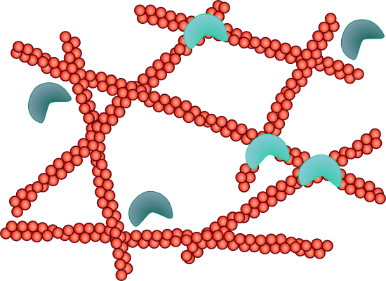
Figure 1: Sketch of a transiently crosslinked polymer network. In thermal equilibrium, some polymer-polymer contacts are crosslinked (bright circle segments), while other crosslinkers are unbound (dark circle segments). For simplicity, we use a reduced description where direct polymer-polymer contacts react by effective first-oder kinetics.

2.3 The inelastic Glassy Wormlike Chain

The glassy wormlike chain (GWLC) model is a phenomenological extension of the wormlike chain (WLC) model, which is the standard model for individual semiflexible polymers such as DNA or F-actin. For an introduction to the GWLC, see Ref. 16. A detailed description of the inelastic GWLC is given in Ref. 35.

In the weakly bending rod approximation, i.e. if thermal forces do not bend the polymer too strongly, the WLC can be solved analytically by a mode decomposition ansatz for the transverse deflections from the straight ground state. The individual modes with index $n$ decay exponentially with a time constant $\tau_{n}$. The GWLC rests on the phenomenological assumption that the relaxation of modes with wavelength $\lambda_{n}$ larger than the mean bond distance $\Lambda$ is slowed down, because $\lambda_{n}/\Lambda-1$ free energy barriers have to be overcome for the mode to relax. Formally, this is expressed by a stretching of the mode relaxation times,

$$\tau_{n}\to\tilde{\tau}_{n}=\left\{\begin{array}[]{c c}\tau_{n}&\lambda_{n}<\Lambda\\ \tau_{n}\exp\left[\mathcal{E}(\lambda_{n}/\Lambda-1)\right]&\lambda_{n}\geq\Lambda\end{array}\right..$$ (10)

In the limit of large free-energy barriers $\mathcal{E}$, the viscoelastic response of the GWLC resembles that of a power-law fluid with exponent ³ $3\mathcal{E}^{-1}$.

In the equilibrium GWLC model, the mean distance $\Lambda$ between polymer-polymer junctions is taken to be a constant $\Lambda_{0}$, unaffected by the equilibrium bond fluctuations. The inelastic GWLC keeps track of forced inelastic bond breaking in the network by dynamically updating $\Lambda$ if the mean fraction $\nu$ of closed bonds in the network changes: $\Lambda(t)=\Lambda_{0}/\nu(t)$. In the simplest version of the inelastic GWLC, the dynamics of the bond network is approximated by an effective first-order kinetics and given by the model presented in section 2.1. See figure 1 for an artistic sketch of the physical picture.

3 Results

3.1 Apparent linear response of a transiently crosslinked power-law fluid

To gain some analytical insights, we examine the influence of bond breaking on the linear response of a schematic power-law fluid, as outlined in section 2.2, equations (8)-(9). To this end, we first assume that both the bonds as well the material in the absence of bond breaking exhibit a linear response. For the sinusoidal driving force in equation (4), the displacement response can be written as

$$x(t) = \frac{G_{0}^{-1}\hat{f}\omega^{-\delta}}{\nu_{0}-\hat{f}\cdot(\alpha_{\nu}^{\prime}(\omega_{0})\sin(\omega_{0}t)-\alpha_{\nu}^{\prime\prime}(\omega_{0})\cos(\omega_{0}t))}$$ (11)

$$\times\left(\sin(\omega_{0}t)-\tan(\delta\pi/2)\cos(\omega_{0}t)\right),$$

where $\nu_{0}$ is the steady-state bond fraction in the absence of driving. If we expand the right-hand side to first oder in $\hat{f}$, we obtain

$$x(t)\approx\frac{G_{0}^{-1}\hat{f}\omega^{-\delta}}{\nu_{0}}\left(\sin(\omega_{0}t)-\tan(\delta\pi/2)\cos(\omega_{0}t)\right),$$

i.e. the bond breaking does not contribute to the linear response.

This suggests that the interpretation for the peaked dissipative patterns observed in Refs. 31, 32, 33 in terms of bond-breaking is not compatible with linear response. To see how nonlinear effects can enter the apparent linear response, we note that it is common practice to extract rheological spectra from a weakly nonlinear response by Fourier-transforming the response and extracting the contribution in resonance with the driving to reconstruct a fictitious sinusoidal response with well-defined amplitude and phase shift (see figure 2 for a somewhat exaggerated example). As nonlinear processes generally excite higher harmonics but also change the resonance response, this practice is bound to include a nonlinear bycatch.

$\begin{array}[]{c@{\hspace{3 mm}}c}\lx@intercol\mbox{\bf\Large a}\hfil\lx@intercol&\lx@intercol\mbox{\bf\Large b}\hfil\lx@intercol\\[-12.23447pt] \hfil\hskip 8.53581pt\\ \includegraphics[width=170.71652pt]{figure2a.pdf}\hfil\hskip 8.53581pt&\includegraphics[width=170.71652pt]{figure2b.pdf}\\[11.38092pt] \hfil\hskip 8.53581pt\\ \end{array}$

Figure 2: Weakly nonlinear response of the inelastic power-law fluid (red solid line) and the corresponding apparent linear response (blue dashed line), reconstructed as described in the main text, displayed over driving force (panel a) and time (panel b). Parameters are $\hat{f}\Delta x_{b}=0.35$, $\delta=0.05$, $\omega\approx k$. Nonlinear effects in the rheology can already be seen for much smaller amplitudes.

In the following, we determine the nonlinear contributions to the apparent linear susceptibilities by calculating the nonlinear response and isolating the contributions in resonance with the driving frequency. In order to do this in a formally fully consistent way, we would need to include higher-order terms for the bond response and for the material response in the absence of bond breaking. However, for our present purpose, which is to capture the essential physics of the model rather than to deal with some circumstantial details, this is in fact not necessary. We therefore assume favorable conditions, namely that both the bonds and the material in the absence of bond breaking react linearly, and that the only relevant source of nonlinearity lies in their mutual interaction. Deviations from our results due to an actually nonlinear bond response and due to potential mechanical nonlinearities in the employed viscoleastic model (here the power-law fluid) can be evaluated numerically if need arises. Their main effect will typically be a mere parameter renormalization.

With these remarks in mind, we can use equation (11) and expand it to higher order in $\hat{f}$. Up to third order and using the abbreviation $d=\tan(\delta\pi/2)$, the expansion reads

$$x(t) \approx \omega_{0}^{-\delta}\frac{\hat{f}}{G_{0}\nu_{0}}\left(\sin(\omega_{0}t)-d\cos(\omega_{0}t)\right)$$

$$+ G_{0}^{-1}\omega_{0}^{-\delta}\left(\frac{\hat{f}}{\nu_{0}}\right)^{2}\left\{\sin(\omega_{0}t)-d\cos(\omega_{0}t)\right\}\left\{\alpha_{\nu}^{\prime}\sin(\omega_{0}t)-\alpha_{\nu}^{\prime\prime}\cos(\omega_{0}t)\right\}$$

$$+ G_{0}^{-1}\omega_{0}^{-\delta}\left(\frac{\hat{f}}{\nu_{0}}\right)^{3}\left\{\sin(\omega_{0}t)-d\cos(\omega_{0}t)\right\}\left\{\alpha_{\nu}^{\prime}\sin(\omega_{0}t)-\alpha_{\nu}^{\prime\prime}\cos(\omega_{0}t)\right\}^{2},$$

with the equilibrium bond fraction $\nu_{0}=(1+e^{-U})^{-1}$. By rewriting the trigonometric functions one can show that the terms of order $\hat{f}^{2}$ only induce a response at the first harmonic at $2\omega_{0}$ and a constant offset. Therefore, the first contribution to the apparent linear response comes from the third-order terms. Dropping all terms that do not contribute to the response at $\omega_{0}$, the apparent linear response becomes

$$x^{(3)} \approx \omega_{0}^{-\delta}\frac{\hat{f}}{G_{0}\nu_{0}}\left(\sin(\omega_{0}t)-d\cos(\omega_{0}t)\right)$$ (13)

$$+ G_{0}^{-1}\omega_{0}^{-\delta}\left(\frac{\hat{f}}{\nu_{0}}\right)^{3}\frac{1}{4}\times$$

$$\big{\{} \left[3\alpha_{\nu}^{\prime}(\omega_{0})^{2}-\alpha_{\nu}^{\prime\prime}(\omega_{0})^{2}-2d\alpha_{\nu}^{\prime}(\omega_{0})\alpha_{\nu}^{\prime\prime}(\omega_{0})\right]\sin(\omega_{0}t)$$

$$-\left[d\alpha_{\nu}^{\prime}(\omega_{0})^{2}+3d\alpha_{\nu}^{\prime\prime}(\omega_{0})^{2}+2\alpha_{\nu}^{\prime}(\omega_{0})\alpha_{\nu}^{\prime\prime}(\omega_{0})\right]\cos(\omega_{0}t)\big{\}}.$$

The apparent linear susceptibility belonging to this response has the real and imaginary parts

$$\alpha^{(3)^{\prime}}(\omega_{0})=\frac{\omega_{0}^{-\delta}}{G_{0}\nu_{0}}\left\{1-\frac{1}{4}\left(\frac{\hat{f}}{\nu_{0}}\right)^{2}\left[\alpha_{\nu}^{\prime\prime}(\omega_{0})^{2}+2d\alpha_{\nu}^{\prime}(\omega_{0})\alpha_{\nu}^{\prime\prime}(\omega_{0})-3\alpha_{\nu}^{\prime}(\omega_{0})^{2}\right]\right\}$$ (14)

and

$$\alpha^{(3)^{\prime\prime}}(\omega_{0})=\frac{\omega_{0}^{-\delta}}{G_{0}\nu_{0}}\left\{d+\frac{1}{4}\left(\frac{\hat{f}}{\nu_{0}}\right)^{2}\left[3d\alpha_{\nu}^{\prime\prime}(\omega_{0})^{2}+2\alpha_{\nu}^{\prime}(\omega_{0})\alpha_{\nu}^{\prime\prime}(\omega_{0})+d\alpha_{\nu}^{\prime}(\omega_{0})^{2}\right]\right\}$$ (15)

respectively (figure 3). Obviously, we can isolate the nonlinear bond-breaking contribution by

$$\alpha_{\rm nl,bonds}(\omega_{0})=\frac{\alpha^{(3)}(\omega_{0})-\alpha^{(0)}(\omega_{0})}{\alpha^{(0)}(\omega_{0})},$$ (16)

where $\alpha$ is either $\alpha^{\prime}$ or $\alpha^{\prime\prime}$ and $\alpha^{(0)}(\omega_{0})$ stands for the linear susceptibilities of the material without bond breaking.

$\begin{array}[]{c@{\hspace{3 mm}}c}\lx@intercol\mbox{\bf\Large a}\hfil\lx@intercol&\lx@intercol\mbox{\bf\Large b}\hfil\lx@intercol\\[-12.23447pt] \hfil\hskip 8.53581pt\\ \includegraphics[width=170.71652pt]{figure3a.pdf}\hfil\hskip 8.53581pt&\includegraphics[width=170.71652pt]{figure3b.pdf}\\[11.38092pt] \hfil\hskip 8.53581pt\\ \end{array}$

Figure 3: Nonlinear (symbols) and linearized (lines) susceptibilities (a) and moduli (b) for the inelastic a power-law fluid defined in section 2.2. Due to the bond breaking, a shoulder develops in the in-phase response (blue), and a peak is observed in the out-of-phase response (purple). The parameters are $\delta=0.01$, $k=1.4\times 10^{-2}$, $U=1$, and $\hat{f}\Delta x_{b}=0.35$.

Equation (16) can be discussed analytically. By inspection of equations (14)-(16) we can see that $\alpha^{(3)}$ exhibits the same scaling behavior as equations (6)-(7). In particular, the frequency scale is also set by $k(1+e^{U})$. However, due to the nonlinear combination of $\alpha_{\nu}$ with $\alpha_{\rm S}$ in equation (16), the peak of the dissipative nonlinear combined response, $\alpha^{(3)^{\prime\prime}}(\omega)$, will in general not be located at $\omega=k(1+e^{U})$. A simple calculation (see appendix) reveals that the position of the peak is at

$$\omega^{*}\approx\frac{1}{\sqrt{3}}k\cdot(1+e^{U}).$$ (17)

$\begin{array}[]{c@{\hspace{3 mm}}c}\lx@intercol\mbox{\bf\Large a}\hfil\lx@intercol&\lx@intercol\mbox{\bf\Large b}\hfil\lx@intercol\\[-12.23447pt] \hfil\hskip 8.53581pt\\ \includegraphics[width=170.71652pt]{figure4a.pdf}\hfil\hskip 8.53581pt&\includegraphics[width=170.71652pt]{figure4b.pdf}\\[11.38092pt] \hfil\hskip 8.53581pt\\ \end{array}$

Figure 4: Position of the peak in the imaginary part of the nonlinear susceptibility. Numerical evaluations for the power-law fluid (blue squares) compared to numerical evaluations for the inelastic GWLC (red circles, see section 3.2) and the analytical prediction, equation (17) (solid lines) and the semi-phenomenological correction, equation (18) (dashed lines, see main text), for various values of the equilibrium off rate $k$ (panel a, $10^{-8}<k<0.1$) and the equilibrium relative binding affinity $e^{U}$ (panel b, $0<e^{U}\leq 64$). The driving amplitude was $\hat{f}\Delta x_{b}=0.12$, other parameters as in figure 3. For the numerical Euler scheme, the time step was chosen as $(2\pi)^{-1}\omega_{0}\Delta t=5\times 10^{-5}$.

This approximate nonlinear formula gives us an analytical prediction (without any free parameter) of the position of the peak in the spectrum in dependence of the bond parameters. To assess the quality of the analytical prediction for the peak position, we numerically evaluate equations (1)-(4) (using an Euler scheme) together with equation (9) (an example is provided in figure 3) and extract the peak frequency for various values of either $k$ or $U$, keeping all other parameters constant. The results are presented in figure 4. We find that the functional dependence is predicted correctly, but that the theoretical predictions are off by a constant factor of about $0.6$ (figure 4b). This is so because we assumed the bonds to always respond linearly and neglected the second-order contribution to the bond response, which actually also contributes to the third order of the displacement response. If one is interested in quantitative parameter estimations, it is straightforward to take into account the second-order contribution. However, the more extended formula is rather cumbersome. In practical applications, additional nonlinear corrections are more conveniently taken into account by a phenomenological correcting factor. Multiplying $e^{U}$ on the right-hand side of equation (17) by $0.64$,

$$\omega^{*}\approx\frac{1}{\sqrt{3}}k\cdot(1+0.64e^{U}),$$ (18)

leads to a good quantitative agreement with the numerical results for a broad range of $k$ and $e^{U}$, (figure 4, dashed lines), independently of the driving force amplitude $\hat{f}$ for $\hat{f}\Delta x_{b}\lesssim 0.18$ (see supplementary figure 1).

The amplitude of the absorption peak turns out to be much more sensitive to the intrinsic nonlinearity of the bond dynamics. Deriving a simple approximate formula as for the peak position is therefore much less useful. Nevertheless, we can predict the approximate dependence on some key parameters from the more complicated, fully consistent expressions. Here we only mention that the amplitude is independent of the equilibrium off rate $k$, depends on the relative affinity as $(1+e^{U})^{-1}$ and depends quadratically on the driving force amplitude $\hat{f}$ (data not shown). We further note that it is easy to show from the analytic equations that asymptotically, for low frequencies, both the in-phase and the out-of-phase part of the susceptibility are merely shifted from the linear-response to higher values, where the shift is stronger for the in-phase susceptibility (see figure 3). The interpretation is that the network softens, while the dissipation increases due to forced bond-breaking. Note that the high-frequency response is not affected by bond breaking, while the low-frequency power-law asymptotics violates the Kramers-Kronig relations, testifying the nonlinear character of the modulus.

3.2 Apparent linear response in the inelastic GWLC model

The inelastic power-law fluid analyzed in the preceding section is to be understood as a schematic model for weakly crosslinked biopolymer networks. A more realistic but still minimalistic description is given by the recently proposed model of an inelastic glassy wormlike chain ³⁵ that builds on the linear modulus of the phenomenologically highly successful glassy wormlike chain (GWLC) model ^{3, 16, 48} and combines it with a bond kinetics scheme as outlined in section 2.3. Due to the slightly more complex structure of the GWLC modulus compared to the power-law fluid, we resort to numerical evaluations to explicitly work out the response. We can again compare these numerical results to the analytical predictions obtained above to better assess the plausible range of validity of our analytical expressions in applications to biopolymer networks.

As established above for the inelastic power-law fluid, bond breaking matters only for the nonlinear response. We therefore again operationally define a set of apparent linear moduli by isolating the resonance with the driving frequency in the Fourier spectrum of the response. Evaluating the nonlinear response of the inelastic GWLC as described in Ref. 35 and calculating the apparent linear moduli for oscillatory stress control, we find a qualitative agreement with measurements on crosslinked actin networks ^{31, 32, 33, 49}. In particular, we find again a maximum in the loss modulus and a shoulder in the storage modulus as illustrated in figure 5.

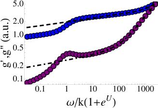
Figure 5: Apparent linear storage (blue) and loss (purple) modulus versus frequency (arbitrary units). The lines represent the strictly linear viscoelastic storage and loss modulus in the absence of bond breaking. The parameters are $k=1.4\times 10^{-2}$, $U=-1$, and $\hat{f}\Delta x_{b}=0.15$.

It is apparent from figure 5 that the frequency dependence of the linear moduli superimposes with the bond effects in a first approximation. Therefore, we can easily isolate the nonlinear part of the response (see section 3.1). To numerically extract the parameter dependence, we evaluate the nonlinear frequency-dependent response of the inelastic GWLC at various values of either $k$ or $U$, keeping all other parameters constant (figures 4 and 6). There are essentially two routes to change $k$ (see sections 2.1 and 2.3), one assuming that changing $k$ also affects the linear modulus of the GWLC (by changing the barrier height $\mathcal{E}$) and one that leaves the linear modulus unaffected (assuming that only the microscopic attempt rate $\tau_{0}^{-1}$ or the bond stiffness changes). Numerical evaluations show that both routes lead to the same results for the peak positions within numerical tolerance (see supplementary figure 2). In contrast, changing $U$ always influences the linear modulus, because $U$ affects equilibrium properties such as the steady-state bond fraction.

$\begin{array}[]{c@{\hspace{3 mm}}c}\lx@intercol\mbox{\bf\Large a}\hfil\lx@intercol&\lx@intercol\mbox{\bf\Large b}\hfil\lx@intercol\\[-12.23447pt] \hfil\hskip 8.53581pt\\ \includegraphics[width=170.71652pt]{figure6a.pdf}\hfil\hskip 8.53581pt&\includegraphics[width=170.71652pt]{figure6b.pdf}\\[11.38092pt] \hfil\hskip 8.53581pt\\ \end{array}$

Figure 6: Apparent linear rheology of an inelastic GWLC. Frequency-dependent loss modulus for various values of $k$ (panel a, $10^{-8}<k<0.1$, increasing from left to right) and for various values of the relative binding affinity $e^{U}$ (panel b, $0<e^{U}\leq 10$, increasing from bottom to top), all other parameters as in figure 5.

The numerical evaluation of the inelastic GWLC in figure 6 clearly reveals the dependence of the peak position on the parameters. In the case of a strongly frequency-dependent or very large modulus (fig 6b), the dissipation due to bond-breaking may be insufficient to become clearly discernible in the rheological spectra, but it can always be uncovered by the subtraction scheme given in equation (16).

The actual position of the peak in dependence on $k$ (figure 4 a) and $e^{U}$ (figure 4 b) obeys the prediction, equation (18), from the analytical calculations in section 3.1 very well (note that we do not have any free parameters to adjust). Most strikingly, the numerical values for $\omega^{*}$ for the inelastic GWLC agree within the numerical error with the numerical values for the inelastic power-law fluid, indicating that the dissipative pattern is reasonably robust. Its characteristic properties are dominated by the generic bond breaking mechanism and relatively insensitive to details of the rheology of the uncrosslinked polymer solution.

3.3 Exemplary application to actin/$\alpha$-actinin networks

Our analytical prediction for the position of the peak in equation (18) is sufficient to extract valuable kinetic information from bulk rheological measurements. While, in principle, one could also exploit the information encoded in the peak amplitude, this would require a more sophisticated fitting procedure taking into account detailed experimental information on the nonlinearity of the response. As this information in not available for pertinent published data, we restrict the following analysis to an interpretation of the peak position, which depends on the equilibrium off rate and the relative affinity, with equation (18). To exemplify the procedure, we use data for an in vitro reconstituted actin/$\alpha$-actinin network⁴⁹, where a peak in the apparent linear loss modulus was observed.

Assuming power-law rheology to be a valid model for the (strictly) linear response, we first use the high-frequency data for $g^{\prime}$ to estimate $G_{0}\nu_{0}$ and $\delta$ to $4.7$ and $0.11$, respectively. Next, we use equation (9) to calculate the linear loss modulus $\alpha^{(0)^{\prime\prime}}$. Then, we use equation (16) to isolate the peak, which turns out to be located at $\omega^{*}\approx 2s^{-1}$. Using an affinity value from the biochemical literature ⁵⁰, $K=2.5\times 10^{6}M^{-1}$, together with actin and $\alpha$-actinin concentrations of $c_{A}=23.8\mu M$ and $c_{\alpha}=0.238$, respectively ⁴⁹, we obtain $e^{U}=K(c_{A}+c_{\alpha})\approx 60$.

From equation (18), we find an equilibrium off rate of $k\approx 0.09s^{-1}$, which agrees with the value obtained for $\alpha$-actinin/actin in mechanical single-molecule experiments ⁴⁷ within the experimental uncertainty. Since our analysis is based on a simple (Bell-type ³⁶) bond-breaking model the numerical agreement should not be over-interpreted, but is certainly reassuring. Note that the rate obtained via either route is a factor of five smaller than values obtained biochemically ⁵⁰. It has been argued that this discrepancy could be due to the restriction of the reaction coordinate by directional loads in single-molecule experiments ⁴⁷. However, we noted an interesting fact that may or may not be a systematic feature. If we follow experimental hints from actin/HMM solutions that $\omega^{*}$ is approximately independent of actin- and crosslinker concentration ³³ and consider the concentration values of $c_{A}=2\mu M$ and $c_{\alpha}=3\mu M$ used in the biochemical bulk measurement ⁵⁰, we obtain $k\approx 0.4s^{-1}$, which is exactly the value reported. This would suggest that the equilibrium off rate depends on either the actin- or the crosslink concentration. Another possible explanation could be that different types of $\alpha$-actinin have been used or that biochemical and biomechanical rate measurements systematically differ by a factor, which cancels out when taking the ratio of the rates to calculate the affinity. This problem certainly deserves a dedicated experimental investigation testing the various hypotheses and possibly involving more elaborate models of bond breaking ^{43, 44}, which is beyond the scope of the present contribution.

4 Conclusions

We have put forward a simple mechanistic model for the weakly nonlinear rheology of reversibly crosslinked biopolymer networks. We verified our analytical predictions against numerical results from two generic models for the viscoelastic response of biopolymer solutions and networks and found good agreement. Thereby, we established the characteristic dissipative pattern due to bond breaking as a robust and reproducible rheological signature of transiently crosslinked biopolymer solutions with well-defined crossliker kinetics. The model seems suitable to explain some puzzling features in the frequency-dependent rheology of crosslinked actin networks in terms of the underlying physics and demonstrate the non-Maxwellian nature of what could easily be mistaken for a classical terminal relaxation pattern in a limited frequency interval.

There are two main conclusions to be drawn from the results presented above. First, the non-trivial rheology of transiently crosslinked biopolymer networks as observed in Refs. 32, 33, 49 can also be found in a conceptually very simple model of an inelastic biopolymer model, the inelastic GWLC. This supports the expectation that the inelastic GWLC is indeed a suitable minimal model for weakly crosslinked biopolymer networks. Second, as the frequency-dependence of the maximum in the loss modulus is very well predicted by our perturbation theory, it seems plausible that the mechanism put forward in section 3.1 is suitable for deducing information on the crosslinker kinetics from the rheological spectra. In doing so, one implicitly acknowledges the intrinsically nonlinear character of the absorption peaks revealed by our analysis.

Compared to single-molecule assays, which provide an alternative method to probe crosslinker properties ⁴⁷, rheology has the advantage of being an ensemble method. A potential caveat of the outlined method is that the procedure to extract the kinetic information from the modulus relies on the knowledge of the linear modulus in the absence of bond breaking (see section 3.1). This information may sometimes be experimentally inaccessible, e.g. if true linear response conditions are technically difficult to realize. However, we discussed the nonlinear rheology for two generic models for the linear viscoelastic response of biopolymer solutions and networks, and we anticipate that for most practical applications at least one of them will provide a reasonable approximation.

The results presented in this paper thus help to turn a widespread speculation about the physical mechanism providing biopolymer networks (and possibly also living cells) with their extraordinary mechanical properties into a concise quantitative prediction amenable to detailed experimental investigation.

Appendix A Peak position in the nonlinear response

Using the abbreviations $x=\omega/(1+e^{U})k$, $h(x)=\alpha_{\rm nl,bonds}^{\prime\prime}$, $b=((\Delta x_{b}+\Delta x_{u})/(4\cosh^{2}(U/2))\cdot\hat{f}/\nu_{0})^{2}$, and $d=\pi/2\tan(\delta)$, equation (16) becomes

$$h(x)=\frac{3bd}{4}\left(\frac{x}{1+x^{2}}\right)^{2}+\frac{b}{2}\frac{x}{(1+x^{2})^{2}}+\frac{bd}{4}\frac{1}{(1+x^{2})^{2}}.$$ (19)

The peak position $x^{*}$ is determined by the condition

$$\frac{d}{dx}h(x)\bigg{|}_{x=x^{*}}=0.$$ (20)

After some simple algebra, equations (19) and (20) yield the condition

$$x^{*3}+\frac{x^{*2}}{d}-\frac{1}{3}x^{*}-\frac{1}{3d}=0.$$ (21)

For $d>0$, this equation has only one positive real solution, $x^{*}=1/\sqrt{3}$. Noting that $x^{*}=\omega^{*}/(1+e^{U})k$, we obtain equation (17) for the frequency of the peak.

References

- Discher et al. 2005 D. E. Discher, P. Janmey and Y.-L. Wang, Science, 2005, 310, 1139–43
- Yeung et al. 2005 T. Yeung, P. C. Georges, L. A. Flanagan, B. Marg, M. Ortiz, M. Funaki, N. Zahir, W. Y. Ming, V. Weaver and P. A. Janmey, Cell. Motil. Cytoskeleton, 2005, 60, 24–34
- Semmrich et al. 2007 C. Semmrich, T. Storz, J. Glaser, R. Merkel, A. R. Bausch and K. Kroy, Proc. Natl. Acad. Sci. U. S. A., 2007, 104, 20199–203
- Trepat et al. 2007 X. Trepat, L. Deng, S. S. An, D. Navajas, D. J. Tschumperlin, W. T. Gerthoffer, J. P. Butler and J. J. Fredberg, Nature, 2007, 447, 592–5
- Fernández and Ott 2008 P. Fernández and A. Ott, Phys. Rev. Lett., 2008, 100, 238102
- Krishnan et al. 2009 R. Krishnan, C. Y. Park, Y.-C. Lin, J. Mead, R. T. Jaspers, X. Trepat, G. Lenormand, D. Tambe, A. V. Smolensky, A. H. Knoll, J. P. Butler and J. J. Fredberg, PloS ONE, 2009, 4, e5486
- Hoffman and Crocker 2009 B. D. Hoffman and J. C. Crocker, Annu. Rev. Biomed. Eng., 2009, 11, 259–88
- Fabry et al. 2001 B. Fabry, G. Maksym, J. Butler, M. Glogauer, D. Navajas and J. Fredberg, Phys. Rev. Lett., 2001, 87, 148102
- Fabry 2003 B. Fabry, Respir. Physiol. Neurobiol., 2003, 137, 109–124
- Wang et al. 2002 N. Wang, I. Tolic-Norrelykke, J. Chen, S. M. Mijailovich, J. P. Butler, J. J. Fredberg and D. Stamenović, Am. J. Cell Physiol., 2002, 282, 606–616
- Sunyer et al. 2009 R. Sunyer, X. Trepat, J. J. Fredberg, R. Farré and D. Navajas, Phys. Biol., 2009, 6, 025009
- Chowdhury et al. 2010 F. Chowdhury, S. Na, D. Li, Y.-C. Poh, T. S. Tanaka, F. Wang and N. Wang, Nat. Mater., 2010, 9, 82–8
- Chen et al. 2010 C. Chen, R. Krishnan, E. Zhou, A. Ramachandran, D. Tambe, K. Rajendran, R. M. Adam, L. Deng and J. J. Fredberg, PloS ONE, 2010, 5, e12035
- Gittes and Mackintosh 1998 F. Gittes and F. C. Mackintosh, Phys. Rev. E, 1998, 58, 1241–1244
- Ingber 2003 D. E. Ingber, J. Cell Sci., 2003, 116, 1157–1173
- Kroy and Glaser 2007 K. Kroy and J. Glaser, New J. Phys., 2007, 9, 416
- Bausch and Kroy 2006 A. Bausch and K. Kroy, Nat. Phys., 2006, 2, 231–238
- Liu and Fletcher 2009 A. P. Liu and D. A. Fletcher, Nat. Rev. Mol. Cell Bio., 2009, 10, 644–50
- Loose and Schwille 2009 M. Loose and P. Schwille, J. Struct. Biol., 2009, 168, 143–51
- Wachsstock et al. 1994 D. H. Wachsstock, W. H. Schwarz and T. D. Pollard, Biophys. J., 1994, 66, 801–9
- Xu et al. 1998 J. Xu, A. Palmer and D. Wirtz, Macromolecules, 1998, 31, 6486–6492
- Caspi et al. 1998 A. Caspi, M. Elbaum, R. Granek, A. Lachish and D. Zbaida, Phys. Rev. Lett., 1998, 80, 1106
- Gardel et al. 2006 M. Gardel, J. Hartwig and F. Nakamura, Proc. Nat. Acad. Sci. U.S.A., 2006, 103, 1762–1767
- Lieleg et al. 2010 O. Lieleg, M. M. A. E. Claessens and A. R. Bausch, Soft Matter, 2010, 6, 218
- Loisel et al. 1999 T. Loisel, R. Boujemaa, D. Pantaloni and M. Carlier, Nature, 1999, 401, 613–616
- Schaller et al. 2010 V. Schaller, C. Weber, C. Semmrich, E. Frey and A. R. Bausch, Nature, 2010, 467, 73–77
- Geiger et al. 2009 B. Geiger, J. P. Spatz and A. D. Bershadsky, Nat. Rev. Mol. Cell Bio., 2009, 10, 21–33
- Fernandez et al. 2007 P. Fernandez, L. Heymann, A. Ott, N. Aksel and P. A. Pullarkat, New J. Phys., 2007, 9, 419
- Gardel et al. 2006 M. L. Gardel, F. Nakamura, J. Hartwig, J. C. Crocker, T. P. Stossel and D. A. Weitz, Phys. Rev. Lett., 2006, 96, 88102
- Koenderink et al. 2009 G. H. Koenderink, Z. Dogic, F. Nakamura, P. M. Bendix, F. C. MacKintosh, J. H. Hartwig, T. P. Stossel and D. A. Weitz, Proc. Natl. Acad. Sci. U. S. A., 2009, 106, 15192–7
- Tharmann et al. 2007 R. Tharmann, M. M. A. E. Claessens and A. R. Bausch, Phys. Rev. Lett., 2007, 98, 088103
- Lieleg et al. 2008 O. Lieleg, M. Claessens, Y. Luan and A. Bausch, Phys. Rev. Lett., 2008, 101, 108101
- Lieleg et al. 2009 O. Lieleg, K. M. Schmoller, M. M. A. E. Claessens and A. R. Bausch, Biophys. J., 2009, 96, 4725–32
- Fletcher and Geissler 2009 D. A. Fletcher and P. L. Geissler, Annu. Rev. Phys. Chem., 2009, 60, 469–86
- Wolff et al. 2010 L. Wolff, P. Fernandez and K. Kroy, New J. Phys., 2010, 12, 053024
- Bell 1978 G. Bell, Science, 1978, 200, 618–627
- Evans and Ritchie 1997 E. Evans and K. Ritchie, Biophys. J., 1997, 72, 1541–1555
- Nguyen-Duong et al. 2003 M. Nguyen-Duong, K. Koch and R. Merkel, Europhys. Lett., 2003, 61, 845–851
- Hummer and Szabo 2003 G. Hummer and A. Szabo, Biophys. J., 2003, 85, 5–15
- Dudko et al. 2006 O. Dudko, G. Hummer and A. Szabo, Phys. Rev. Lett., 2006, 96, 1–4
- Walton et al. 2008 E. B. Walton, S. Lee and K. J. Van Vliet, Biophys. J., 2008, 94, 2621–30
- Dudko et al. 2008 O. K. Dudko, G. Hummer and A. Szabo, Proc. Natl. Acad. Sci. U. S. A., 2008, 105, 15755–60
- Tshiprut et al. 2008 Z. Tshiprut, J. Klafter and M. Urbakh, Biophys. J., 2008, 95, L42–4
- Freund 2009 L. B. Freund, Proc. Natl. Acad. Sci. U. S. A., 2009, 106, 8818–23
- Kramers 1940 H. Kramers, Physica, 1940, VII, 284–304
- Hoffman et al. 2007 B. Hoffman, G. Massiera and J. Crocker, Phys. Rev. E, 2007, 76, 051906
- Ferrer et al. 2008 J. M. Ferrer, H. Lee, J. Chen, B. Pelz, F. Nakamura, R. D. Kamm and M. J. Lang, Proc. Natl. Acad. Sci. U. S. A., 2008, 105, 9221–9226
- Glaser et al. 2008 J. Glaser, O. Hallatschek and K. Kroy, Eur. Phys. J. E, 2008, 26, 123–36
- Broedersz et al. 2010 C. P. Broedersz, M. Depken, N. Y. Yao, M. R. Pollak, D. A. Weitz and F. C. MacKintosh, arXiv, 2010, 4
- Goldmann and Isenberg 1993 W. H. Goldmann and G. Isenberg, FEBS Lett., 1993, 336, 408–10