Energy transport and fluctuations in small conductors

Abstract

The Landauer-Büttiker formalism provides a simple and insightful way for investigating many phenomena in mesoscopic physics. By this approach we derive general formulas for the energy currents and apply them to the basic setups. Of particular interest are the noise properties. We show that energy current fluctuations can be induced by zero-point fluctuations and we discuss the implications of this result.

I Introduction

The study of quantum effects in small conductors is generally referred to as mesoscopic physics. The wave nature of the electrons is relevant and many counterintuitive results appear: the quantization of the conductance, persistent currents in small loops, the quantum Hall effect and the weak localization effect, to cite but a few (for a review see Ref. datta and references therein). In the Landauer-Büttiker formalism the motion of the electrons in the conductors is described as a scattering process. This approach was originally proposed to investigate the conductance of a single-channel wire landauer1 ; landauer2 and then extended to other structures ring ; channels ; terminals ; hall and properties noise_1990 ; noise_1992 ; review ; pretre . Instead, much less interest have received the thermoelectric properties. The first investigations of energy transport in mesoscopic conductors appeared in Refs. anderson ; imry_thermo ; streda . The average properties were studied also in Refs. butcher ; guttman , while the noise properties in Ref. krive . In this paper we extend the Landauer-Büttiker formalism to account for energy transport and fluctuations. We derive the energy counterpart of several results characterizing the electrical properties of mesoscopic conductors. The role of irreversible processes is at the center of our attention, especially in equilibrium at low temperatures. In this regime we show that in a two-terminal conductor energy exchange can happen, of course, under the constraint of no net flow of energy.

II General results

The model. We consider a multi-terminal many channel coherent conductor. This means that the energy carriers can enter or leave the sample through $M$ leads with $N_{\alpha}$ transverse channels, $\alpha=1,\ldots,M$, and their motion from one lead to another is phase coherent. Each lead is connected to an electron reservoir characterized by the temperature $T_{\alpha}$, the chemical potential $\mu_{\alpha}$ and the Fermi-Dirac distribution function $f_{\alpha}(E)=\{\exp((E-\mu_{\alpha})/k_{\mathrm{B}}T_{\alpha})+1\}^{-1}$, where $k_{\mathrm{B}}$ is the Boltzmann constant. The reservoirs absorb all incident electrons irrespective of their phase and energy. Furthermore, the reservoirs are incoherent, that is, the electrons emerging from different reservoirs do not have any phase relationship and their phase is also independent of that of absorbed electrons. We neglect any interaction of the electrons with other electrons or with phonons, magnetic impurities, et cetera. At the conductor elastic scattering processes take place. The elastic scattering properties of the conductor are described by the scattering matrix $\bm{S}$. It relates the amplitude of the outgoing states to the amplitude of the incoming states. Let $\bm{S}_{\alpha\beta}(E)$ be the submatrix of dimension $N_{\alpha}\times N_{\beta}$ defined as $\big{(}\bm{S}_{\alpha\beta}(E)\big{)}_{mn}=S_{\alpha\beta,mn}(E)$, $m=1,\ldots,N_{\alpha}\ \text{and}\ n=1,\ldots,N_{\beta}$. $\bm{S}_{\alpha\beta}(E)$ connects the incident amplitudes in lead $\beta$ to the outgoing amplitudes in lead $\alpha$. An energy carrier arriving at the conductor in contact $\beta$ in channel $n$ has probability $R_{\beta\beta,mn}=\mid S_{\beta\beta,mn}\mid^{2}$ to be scattered back into contact $\beta$ in channel $m$ and probability $T_{\alpha\beta,mn}=\mid S_{\alpha\beta,mn}\mid^{2}$ to be scattered into contact $\alpha$ in channel $m$. Evidently, for a carrier in contact $\beta$ the total probability of reflection and of transmission into contact $\alpha$ are given by, respectively, $R_{\beta\beta}=\sum_{mn}R_{\beta\beta,mn}=\sum_{mn}\mid S_{\beta\beta,mn}\mid^{2}=\mathrm{Tr}(\bm{S}^{{\dagger}}_{\beta\beta}\bm{S}_{\beta\beta})$ and $T_{\alpha\beta}=\sum_{mn}T_{\alpha\beta,mn}=\sum_{mn}\mid S_{\alpha\beta,mn}\mid^{2}=\mathrm{Tr}(\bm{S}^{{\dagger}}_{\alpha\beta}\bm{S}_{\alpha\beta})$ ; $\mathrm{Tr}$ stands for trace. The conservation of the energy carriers imposes that $\bm{S}$ is unitary.

Average properties. We assume that the energy carriers are only electrons and we do not take into account the spin degeneracy. The classical expression of the energy current in lead $\alpha$ is given by $W_{\alpha}(t)=(1/e)\int(E-\mu)\mathrm{d}I_{\alpha}(t,E)$. At low temperatures the chemical potential $\mu$ can be assumed to be approximately the energy value above which transport occurs, i.e., the Fermi energy $E_{\mathrm{F}}$. We subtract it from the total energy of the energy carriers since we are interested in the net energy flowing through the leads, to which the Fermi sea does not contribute. With calculations similar to those made in Refs. noise_1990 ; noise_1992 ; review ; pretre , we find that the average energy current in lead $\alpha$ is

$$\langle\hat{W}_{\alpha}(t)\rangle=\frac{1}{h}\sum_{\beta}\int\mathrm{d}E(E-\mu)(N_{\alpha}\delta_{\alpha\beta}-T_{\alpha\beta}(E))f_{\beta}(E)\ ,$$ (1)

where $\delta_{\alpha\beta}$ is the Kronecker delta. We consider the linear response regime, i.e., for all $\beta$ we write $\mu_{\beta}=E_{\mathrm{F}}+\Delta\mu_{\beta}$ and $T_{\beta}=T+\Delta T_{\beta}$. $E_{\mathrm{F}}$ is the Fermi energy of the electrons in the reservoirs and $T$ is approximately the average temperature of the system. When $\Delta\mu_{\alpha}$ and $\Delta T_{\alpha}$ are supposed to be small, we find that we can write the above expression as

$$\langle\hat{W}_{\alpha}(t)\rangle=\sum_{\beta}\Delta\mu_{\beta}K^{\Delta\mu}_{\alpha\beta}+\sum_{\beta}\Delta T_{\beta}K^{\Delta T}_{\alpha\beta}\ ,$$ (2)

with the thermal conductance matrices $K^{\Delta\mu}_{\alpha\beta}$ and $K^{\Delta T}_{\alpha\beta}$ defined as

$$K^{\Delta\mu}_{\alpha\beta}=\frac{1}{h}\int\mathrm{d}E(E-E_{\mathrm{F}})\Big{(}-\frac{\partial f(E)}{\partial E}\Big{)}\big{(}N_{\alpha}\delta_{\alpha\beta}-T_{\alpha\beta}(E)\big{)}$$

and

$$K^{\Delta T}_{\alpha\beta}=\frac{1}{hT}\int\mathrm{d}E(E-E_{\mathrm{F}})^{2}\Big{(}-\frac{\partial f(E)}{\partial E}\Big{)}\times\\ \big{(}N_{\alpha}\delta_{\alpha\beta}-T_{\alpha\beta}(E)\big{)}\ ;$$ (3)

$f(E)=\{\exp((E-E_{\mathrm{F}})/k_{\mathrm{B}}T)+1\}^{-1}$. From Eq. (2) we see that, in the linear response regime, there are two, clearly independent, contributions to energy transport due to a temperature or a chemical potential gradient. In the zero temperature limit, of course, one has to use Eq. (1), as we shall see in the next section.

Fluctuations. The spectral density of energy current fluctuations $S_{\alpha\beta}^{W}$ is defined by

$$2\pi S_{\alpha\beta}^{W}(\omega)\delta(\omega+\omega^{\prime})=\\ \langle\Delta\hat{W}_{\alpha}(\omega)\Delta\hat{W}_{\beta}(\omega^{\prime})+\Delta\hat{W}_{\beta}(\omega^{\prime})\Delta\hat{W}_{\alpha}(\omega)\rangle\ .$$ (4)

We indicate by $\Delta\hat{W}_{\alpha}(\omega)=\hat{W}_{\alpha}(\omega)-\langle\hat{W}_{\alpha}(\omega)\rangle$ the Fourier transform of the fluctuating part of the energy current operator in lead $\alpha$. We introduce the matrix noise_1992 $\bm{A}_{\beta\gamma}(\alpha,E,E^{\prime})=\mathbb{I}_{\alpha}\delta_{\alpha\beta}\delta_{\alpha\gamma}-\bm{S}_{\alpha\beta}^{{\dagger}}(E)\bm{S}_{\alpha\gamma}(E^{\prime})$; $\mathbb{I}_{\alpha}$ is the identity matrix $\alpha\times\alpha$. By following closely the analysis proposed in Refs. noise_1990 ; noise_1992 ; review , we find that

$$S_{\alpha\beta}^{W}(\omega)=\frac{1}{h}\int\mathrm{d}E\ (E+\frac{\hbar\omega}{2}-\mu)^{2}\times\\ \sum_{\delta\gamma}\mathrm{Tr}\big{(}\bm{A}_{\delta\gamma}(\alpha,E,E+\hbar\omega)\bm{A}_{\gamma\delta}(\beta,E+\hbar\omega,E)\big{)}\times\\ \big{\{}f_{\delta}(E)[1-f_{\gamma}(E+\hbar\omega)]+f_{\gamma}(E+\hbar\omega)[1-f_{\delta}(E)]\big{\}}\ .$$ (5)

From the physical quantities entering this formula we see that energy current noise is determined by the transmission properties of the conductor and the statistics of the energy carriers. It is straightforward to verify that our result satisfies

$$S_{\alpha\beta}^{W}(-\omega)=S_{\beta\alpha}^{W}(\omega)\ .$$ (6)

In the zero-frequency limit there is another useful identity. For the unitarity of the scattering matrix we obtain

$$\sum_{\alpha}S_{\alpha\beta}^{W}(0)=\sum_{\beta}S_{\alpha\beta}^{W}(0)=0\ .$$ (7)

We conclude this section by making the remark that noise evokes the idea of disorder, but $S_{\alpha\beta}^{W}$ is also a measure of the correlation of the deviations away from the average value of the energy current in the leads. Another important point is that noise is determined by both the particle and the wave properties of the energy carriers. Indeed, $S_{\alpha\beta}^{W}$ is derived starting from operators in the second quantization formalism. The details can not be given here exhaustively, but we address the reader to Refs. noise_1992 ; review for analogous calculations.

III Applications

The quantum of thermal conductance. As a first application of our general results, and notably of Eq. (2), we consider a two-terminal conductor. The leads have the same number of channels, $N$, and we suppose that energy transport is due only to a temperature gradient, that is, $\Delta\mu_{1}=\Delta\mu_{2}=0$, $\Delta T_{2}=0$ and $\Delta T_{1}\neq 0$, as shown in Figure 1. In the basis of the eigen-channels and by assuming that the scattering matrix is approximately constant over the energy range where transport occurs, the energy current through the two leads is given by

$$W=\langle\hat{W}_{1}\rangle=-\langle\hat{W}_{2}\rangle=\Delta T_{1}\sum_{n}T_{n}(E_{\mathrm{F}})\times\\ \frac{1}{hT}\int\mathrm{d}E(E-E_{\mathrm{F}})^{2}\Big{(}-\frac{\partial f(E)}{\partial E}\Big{)}\ .$$ (8)

We denote $T_{n}(E_{\mathrm{F}})$ the eigenvalues of the matrix $\textbf{S}^{{\dagger}}_{21}\textbf{S}_{21}$ evaluated at the Fermi energy. They should not be confused with the temperature $T$. At low temperatures the integral in the above result can be estimated. We obtain the quantum of thermal conductance anderson ; rego :

$$K_{\mathrm{o}}(T)=\frac{1}{hT}\int\mathrm{d}E(E-E_{\mathrm{F}})^{2}\Big{(}-\frac{\partial f(E)}{\partial E}\Big{)}\cong\frac{\pi^{2}k_{\mathrm{B}}^{2}}{3h}T\ .$$

If now we apply a small voltage across the conductor, we readily obtain the Wiedemann-Franz law $L=K_{\mathrm{o}}(T)/TG_{\mathrm{o}}=(\pi^{2}/3)(k_{\mathrm{B}}/e)^{2}$, where $G_{\mathrm{o}}=e^{2}/h$ is the quantum of conductance. $L$ is usually referred to as the Lorentz number.

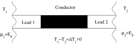
Figure 1: Two-terminal conductor in the presence of a temperature gradient: $T_{1}\neq T_{2}$.

Dissipation and non-equilibrium noise. Let us consider a two-terminal conductor at zero temperature over which a small voltage $V$ is applied. We choose $\Delta\mu_{1}=eV$ and $\Delta\mu_{2}=0$. The leads have the same number of channels. Making use of the Landauer formula, which yields the average current $I=(e^{2}/h)T_{12}V$, and of the unitarity of the scattering matrix, from Eq. (1) we readily obtain $\langle\hat{W}_{1}\rangle=-\langle\hat{W}_{2}\rangle=(1/2)IV$. We immediately see that $\langle\hat{W}_{1}\rangle+\langle\hat{W}_{2}\rangle=0$, and thus the conductor does not absorb energy. This result is usually interpreted as follows. We might write the energy current flowing through the leads as $(I/e)\times eV/2$. $I/e$ represents the flow of particles through the conductor, and $eV/2$ is the average excess energy of the electrons. When an electron enters the sample, it leaves behind a hole with approximately the same energy. In order to obtain the total energy dissipated in the reservoirs we have also to take into account the energy released by holes. This is done by multiplying the energy current in the leads, to which contribute only the electrons, by a factor of $2$. This yields the expected result $IV$. Nevertheless, this analogy with the ohmic behavior is only formal. In mesoscopic conductors we have a spatial separation between elastic and inelastic scattering. Our result of course depends on the geometry of the conductor via its transmissive behavior, but the energy is dissipated in the reservoirs.

Let us come to the energy current noise properties. From Eq. (5), in the basis of eigen-channels, we obtain

$$S_{11}^{W}(0)=\frac{2}{3h}\sum_{n}T_{n}(1-T_{n})(eV)^{3}\ ,$$ (9)

and from Eqs. (6) and (7) we see that $S_{11}^{W}(0)=S_{22}^{W}(0)=-S_{12}^{W}(0)=-S_{21}^{W}(0)$. For completeness, let us point out that in the low transparency limit, i.e. $T_{n}\ll 1$, corresponding for example to the case of a tunnel barrier, we have $S_{11}^{W}(0)=(2/3)(e^{3}/h)\sum_{n}T_{n}\ V^{3}=(2/3)eIV^{2}$, where we have used Landauer formula $G=(e^{2}/h)\sum_{n}T_{n}$ for the conductance, which yields the average current flowing through the conductor $I=GV$. The above result is usually referred to as the classical limit. It corresponds to the case where the emission of electrons is uncorrelated and, as a result, the instants of emission are random and governed by a distribution function of the Poisson type review .

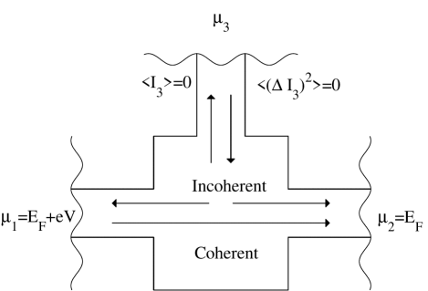
Figure 2: Two-terminal conductor with a voltage probe. A fraction of the energy carriers are scattered coherently and the others incoherently in the forward and backward direction.

Inelastic scattering. We now study the effect of inelastic scattering on energy transport. Within the scattering formalism, neglecting any kind of interaction, it is possible to introduce inelastic scattering by adding a fictitious voltage probe to the mesoscopic conductor inelastic1 , as shown in Figure 2. This model for inelastic scattering has the advantage of reducing the study of inelastic scattering to an elastic scattering problem with the further requirement of local current conservation at the voltage probe. An ideal voltmeter has an infinite internal impedance and therefore at the voltage probe the current vanishes at any moment of time inelastic1 ; inelastic2 : $\langle I_{3}\rangle=\langle(\Delta I_{3})^{2}\rangle=0$. This means that when an electron is absorbed by the voltage probe reservoir its phase and energy are randomized, and immediately another electron is injected into the conductor with an energy and a phase uncorrelated with those of the outgoing electron. The energy current flowing through the conductor has both a coherent and an incoherent component. A fraction of the electrons is scattered coherently from contact $1$ to $2$ and the others are scattered inelastically in the forward and in the backward direction. We concentrate ourselves on the case of completely incoherent transmission, i.e. $T_{21}=T_{12}=0$, and thus $T_{3\alpha}=T_{\alpha 3}$, at zero temperature. By using Eq. (1) we find for the energy current in the three leads

$$\langle\hat{W}_{1}\rangle=\frac{T_{13}}{h}\frac{(eV)^{2}}{2}-\frac{1}{h}\frac{T_{13}T_{31}^{2}}{(T_{31}+T_{32})^{2}}\frac{(eV)^{2}}{2}\ ,$$

$$\langle\hat{W}_{2}\rangle=-\frac{1}{h}\frac{T_{23}T_{31}^{2}}{(T_{31}+T_{32})^{2}}\frac{(eV)^{2}}{2}\ ,$$

$$\langle\hat{W}_{3}\rangle=-\frac{1}{h}\frac{T_{31}T_{32}}{T_{31}+T_{32}}\frac{(eV)^{2}}{2}\ .$$

The unitary of the scattering matrix guarantees that $\langle\hat{W}_{1}\rangle+\langle\hat{W}_{2}\rangle+\langle\hat{W}_{3}\rangle=0$, and so all dissipation processes occur in the reservoirs. Then, the voltage probe reservoir absorbs energy: the electrons entering the voltage probe are thermalized through inelastic scattering and release a fraction of their excess energy. $\langle\hat{W}_{3}\rangle$ is thus nothing but the Joule heat dissipated in the voltage probe (cf. Refs. inelastic1 ; ibm ).

We study instead energy current fluctuations in the quasi-elastic regime. This means that the electron entering the voltage probe is replaced by an electron with the same energy, but an uncorrelated phase jong . This is the reason why this model is generally employed to simulate phase-breaking processes. Energy conservation is achieved by demanding that at the voltage probe current is conserved in each energy interval jong . It is worth noting that phase-breaking processes do not affect the average energy current flowing through the conductor. In fact, we find that $\langle\hat{W}_{1}\rangle=-\langle\hat{W}_{2}\rangle=IV/2$, as obtained for the two-terminal conductor. For the noise properties, from Eq. (5), in the zero-frequency limit, we find that

$$S_{11}^{W}(0)=\frac{2}{3}eIV^{2}\big{[}\frac{e^{2}}{h}\sum_{n}T^{(1)}_{n}(1-T^{(1)}_{n})R_{1}^{4}+\\ \frac{e^{2}}{h}\sum_{n}T^{(2)}_{n}(1-T^{(2)}_{n})R_{2}^{4}+R_{1}^{2}R_{2}+R_{1}R_{2}^{2}\big{]}/R^{3}\ ,$$ (10)

where $T_{n}^{(1)}$ and $T_{n}^{(2)}$ designate the transmission probabilities from contact 1 to 3 and from contact 3 to 2, respectively (see Fig. 2); then, $R=G^{-1}=R_{1}+R_{2}$ is the total resistance of the conductor, with $R_{1}=(h/e^{2})/T_{31}$ and $R_{2}=(h/e^{2})/T_{32}$. As before, $S_{11}^{W}(0)=S_{22}^{W}(0)=-S_{12}^{W}(0)=-S_{21}^{W}(0)$. Interestingly, for a ballistic conductor the above result does not vanish, in contrast to Eq. (9), but reduces to $S_{11}^{W}(0)=(2/3)eIV^{2}R_{1}R_{2}(R_{1}+R_{2})^{-2}$. This indicates that the presence of phase-breaking processes are associated with energy current fluctuations.

Equilibrium noise. We recall that in equilibrium the power spectrum of current fluctuations is given by

$$S^{I}(\omega)=4GE(\omega,T)\ ,\quad\text{where}$$ (11)

$$E(\omega,T)=\frac{\hbar\omega}{2}+\frac{\hbar\omega}{\exp(\hbar\omega/k_{\mathrm{B}}T)-1}\ .$$ (12)

$G$ is the conductance of a two-terminal conductor and $E(\omega,T)$ is the average energy at temperature $T$ of an oscillator of frequency $\omega$, being the sum of the zero-point energy and the Planck spectrum. Equation (11) is known as the fluctuation-dissipation theorem, stating that equilibrium is governed by irreversible processes at the microscopic level causing fluctuations because the system experiences a fluctuating force arising from the interaction with its environment nyquist ; callen . At high temperatures Eq. (12) reduces to the classical equipartition value, indicating that the fluctuating force originates from thermal agitation, while at low temperatures we are left with the quantum of zero-point energy. We want to understand whether vacuum fluctuations are associated with energy exchange. Let us first consider energy current noise at a non-vanishing temperature $T$ in the zero-frequency limit. A simple calculation shows that Eq. (5) yields $S_{\alpha\beta}^{W}(0)=2k_{\mathrm{B}}T^{2}\big{(}K_{\alpha\beta}^{\Delta T}+K_{\beta\alpha}^{\Delta T}\big{)}$. This is the Johnson-Nyquist formula for energy current noise. Now, at zero temperature we find that

$$S_{\alpha\beta}^{W}(\omega)=\frac{2}{3}\frac{1}{e^{2}}(G_{\alpha\beta}+G_{\beta\alpha})\Big{(}\frac{\hbar\mid\omega\mid}{2}\Big{)}^{3}\ .$$ (13)

For clarity we have written the result in terms of the conductance matrix $G_{\alpha\beta}=(e^{2}/h)(N_{\alpha}\delta_{\alpha\beta}-T_{\alpha\beta})$. The only fundamental constant that enters this result is the Planck constant, and we see that energy current noise is proportional to $\hbar^{2}$, in line with what obtained in Ref. nagaev . Equation (13) is the main result of our work. It is interesting to consider the case of a ballistic, single-channel, two-terminal conductor because this situation admits a simple interpretation. We find that $S_{11}^{W}(\omega)=S_{22}^{W}(\omega)=-S_{12}^{W}(\omega)=-S_{21}^{W}(\omega)=(\hbar^{2}/12\pi)\mid\omega\mid^{3}>0$. This means that the energy current fluctuates and if a mode tends to enter the sample in a lead, the same mode tends to leave the sample from the other lead. It also follows that energy transport is forbidden only on the average.

IV Conclusions

Within a unified framework we have investigated energy transport and fluctuations in mesoscopic conductors. Importantly, our results on noise can be of relevance for the debate on dephasing from vacuum fluctuations nagaev ; webb ; zaikin ; cedraschi ; imry_dephasing . In the Landauer-Büttiker formalism there are no fluctuating forces appearing explicitly, but we neglect any kind of interaction in the leads. For this reason, Eq. (13) allows us to conclude that energy exchange between the reservoirs is forbidden only on the average. Finally, the conductor and the leads form a conservative hamiltonian system and ultimately we have shown with an example that the coherence of an open quantum system is not always fully preserved also in equilibrium at very low temperatures.

- (1) S. Datta, Electronic Transport in Mesoscopic Systems, (Cambridge University Press, Cambridge, 1995).
- (2) R. Landauer, IBM J. Res. Dev. 1, 223 (1957).
- (3) R. Landauer, Phil. Mag. 21, 683 (1970).
- (4) R. Landauer and M. Büttiker, Phys. Rev. Lett. 54, 2049 (1985).
- (5) M. Büttiker, Y. Imry, R. Landauer, and S. Pinhas, Phys. Rev. B 31, 6207 (1985).
- (6) M. Büttiker, Phys. Rev. Lett. 57, 1761 (1986).
- (7) M. Büttiker, Phys. Rev. Lett. 62, 229 (1989).
- (8) M. Büttiker, Phys. Rev. Lett. 65, 2901 (1990).
- (9) M. Büttiker, Phys. Rev. B 46, 12485 (1992).
- (10) A. Prêtre, H. Thomas, and M. Büttiker, Phys. Rev. B 54, 8130 (1996).
- (11) Ya.M. Blanter and M. Büttiker, Phys. Rep. 336, 1 (2000).
- (12) H.-L. Engquist and P.W. Anderson, Phys. Rev. B 24, 1151 (1981).
- (13) U. Sivan and Y. Imry, Phys. Rev. B 33, 551 (1986).
- (14) P. Streda, J. Phys. Cond. Matter 1, 1025 (1989).
- (15) P.N. Butcher, J. Phys. Cond. Matter 2, 4869 (1990).
- (16) G.D. Guttman, E. Ben-Jacob, and D.J. Bergman, Phys. Rev. B 53, 15856 (1996).
- (17) I.V. Krive, E.N. Bogachek, A.G. Scherbakov, and U. Landman, Phys. Rev. B 64, 233304 (2001).
- (18) L.G.C. Rego and G. Kirczenow, Phys. Rev. Lett. 81, 232 (1998).
- (19) M. Büttiker, Phys. Rev. B 33, 3020 (1986).
- (20) C.W.J. Beenakker and M. Büttiker, Phys. Rev. B 46, 1889 (1992).
- (21) M. Büttiker, IBM J. Rev. Dev. 32, 317 (1988).
- (22) M.J.M. de Jong and C.W.J. Beenakker, Physica A 230, 219 (1996).
- (23) H. Nyquist, Phys. Rev. 32, 110 (1928).
- (24) H.B. Callen and T.A. Welton, Phys. Rev. 83, 34 (1951).
- (25) K.E. Nagaev and M. Büttiker, Europhys. Lett. 58, 475 (2002).
- (26) P. Mohanty, E.M.Q. Jariwala, and R.A. Webb, Phys. Rev. Lett. 78, 3366 (1997).
- (27) D.S. Golubev and A.D. Zaikin, Phys. Rev. Lett. 81, 1074 (1998).
- (28) P. Cedraschi, V.V. Ponomarenko, and M. Büttiker, Phys. Rev. Lett. 84, 346 (2000).
- (29) D. Cohen and Y. Imry, Phys. Rev. B 59, 11143 (1999).