Gluon saturation and inclusive production at low transverse momenta

Abstract

In this letter we suggest the generalization of $k_{T}$-factorization formula for inclusive gluon production for the dense-dense parton system scattering. It turnes out that the soft gluon production with transverse momentum $p_{T}$ is suppressed by additional Sudakov-like factor that depends on $p^{2}_{T}/Q^{2}_{s}$ ratio in a good agreement with the first numerical calculation in Colour Glass Condensate approach by J. P. Blaizot, T. Lappi and Y. Mehtar-Tan.

It is well known that our approach to inclusive production of an gluon jet is based on $k_{T}$ factorizationKTF1 ; KTF2 ; KTF3 ; KTF4 which leads to

$$\frac{d\sigma}{dy\,d^{2}p_{T}}\,\,=\,\,\frac{2\pi\bar{\alpha}_{s}}{p^{2}_{\perp}}\int d^{2}k_{T}\,\,\phi^{h_{1}}_{G}\left(x_{1};\vec{k}_{T}\right)\,\phi^{h_{2}}_{G}\left(x_{2};\vec{p}_{T}-\vec{k}_{T}\right)$$ (1)

where $\phi^{h_{i}}_{G}$ are the probability to find a gluon that carries $x_{i}$ fraction of energy with $k_{\perp}$ transverse momentum and $\bar{\alpha}_{s}\,=\,\alpha_{s}N_{c}/\pi$ with the number of colours equals $N_{c}$.

In the framework of high density QCDGLR ; MUQI ; MV ; B ; MUCD ; K ; JIMWLK ; KLN ; KLNLHC the $k_{T}$ -factorization has been proven KTINC (see also Refs. BRINC ; CMINC ; KLINC ; LPINC ; KLPINC ) for the scattering of the diluted system of partons, say for virtual photon, with the dense one. Such scattering is characterized by two scale of hardness: the saturation momentum of the dense system $Q_{s}$ and the $p_{T}$ of the produced gluon. The dense-dense parton system scattering has three scales of hardness: two saturation momenta and $p_{T}$; and the $k_{T}$ -factorization has not been proven for this process. The most dangerous region is for $p_{T}$ smaller than both saturation momenta ( $p_{t}\,<\,Q_{1,s}\,\leq\,Q_{2s}$) where we did not expect that $k_{T}$ factorization will work. However, for $Q_{1,s}\,<\,p_{T}\,<\,Q_{2s}$ we are dealing with scattering with two scales of hardness and we can expect that $k_{T}$ factorization is valid here. In this paper we address this problem and suggests the generalization of the $k_{T}$ factorization (see below Eq. (2)) for $p_{t}\,<\,Q_{1,s}\,\leq\,Q_{2s}$.

As it was shown in Ref.KTINC $\phi^{h_{i}}_{G}\left(x_{1};\vec{k}_{\perp}\right)$ can be written through dipole scattering amplitude $N\left(x_{i},r_{\perp};b\right)$, where $r_{\perp}$ is the dipole size and $b$ is the impact parameter of the scattering. This relation reads as follows

$$\phi^{h_{i}}_{G}\left(x_{i};\vec{k}_{T}\right)\,\,=\,\,\frac{1}{\bar{\alpha}_{s}\,4\pi}\,\int d^{2}b\,d^{2}r_{\perp}e^{i\vec{k}_{T}\cdot\vec{r}_{\perp}}\,\,\nabla^{2}_{\perp}\,N^{h_{i}}_{G}\left(y_{i}=\ln(1/x_{i});r_{\perp};b\right)$$ (2)

where

$$N^{h_{i}}_{G}\left(y_{i}=\ln(1/x_{i});r_{\perp};b\right)\,\,=\,\,2\,N\left(y_{i}=\ln(1/x_{i});r_{\perp};b\right)\,\,\,-\,\,\,N^{2}\left(y_{i}=\ln(1/x_{i});r_{\perp};b\right)$$ (3)

$N\left(y_{i}=\ln(1/x_{i});r_{\perp};b\right)$ is the dipole -hadron ($h_{i}$) scattering amplitude which satisfy the Balitsky-Kovchegov equation.

Using that $N\left(x_{i},r_{\perp};b\right)$ is a function of $r^{2}_{\perp}$ we can rewrite Eq. (2) in the form

$$\phi^{h_{i}}_{G}\left(x_{i};\vec{k}_{T}\right)\,\, = \,\,\frac{1}{\bar{\alpha}_{s}\,4\pi}\,\int d^{2}b\,d^{2}r_{\perp}e^{i\vec{k}_{T}\cdot\vec{r}_{\perp}}\frac{1}{r_{\perp}}\,\frac{\partial}{\partial r_{\perp}}\,r_{\perp}\frac{\partial}{\partial r_{\perp}}\,N^{h_{i}}_{G}\left(y_{i}=\ln(1/x_{i});r_{\perp};b\right);\,$$

$$= \,\,\frac{1}{\bar{\alpha}_{s}\,4\pi}\,\int d^{2}b\,\Big{\{}2\pi\Big{(}e^{i\vec{k}_{T}\cdot\vec{r}_{\perp}}\,\,\,r_{\perp}\frac{\partial}{\partial r_{\perp}}\,N^{h_{i}}_{G}\left(y_{i}=\ln(1/x_{i});r_{\perp};b\right)\Big{)}|^{r_{\perp}=\infty}_{r_{\perp}=0}\,\,$$

$$- \,\,ik_{T}\int dr_{\perp}\,d\phi\,\cos\phi e^{ik_{T}r_{\perp}\,\cos\phi}\,r_{\perp}\frac{\partial}{\partial r_{\perp}}\,N^{h_{i}}_{G}\left(y_{i}=\ln(1/x_{i});r_{\perp};b\right)\Big{\}};$$ (5)

At $r_{\perp}\to 0$ the amplitude $N_{G}$ approaches the solution of the DGLAP equation which in our case corresponds the double log limit of the BFKL equation. Therefore

$$\int d^{2}b\,r_{\perp}\frac{\partial}{\partial r_{\perp}}\,N^{h_{i}}_{G}\left(y_{i}=\ln(1/x_{i});r_{\perp};b\right)\,\to\,\mbox{DLA}\,$$ (6)

$$\,\propto\,r_{\perp}\frac{\partial}{\partial r_{\perp}}\,\exp\Big{(}\sqrt{4\bar{\alpha}_{s}\ln(1/x)\,\ln(1/(r^{2}_{\perp}\lambda^{2}_{QCD})}\,-\,\,\,\ln(1/(r^{2}_{\perp}\lambda^{2}_{QCD})\Big{)}\,\,\xrightarrow{r_{\perp}\to 0}\,0$$

It is worth to mention that the impact parameter dependence enters in Eq. (6) as a factor and cannot change our claim that this term vanishes at $r_{\perp}\to 0$.

At large $r_{\perp}$ $1-N_{G}\propto\exp\Big{(}-C\ln^{2}\left(r^{2}Q^{2}_{s}\right)\Big{)}$ (see Ref.LT ) and, therefore,

$$\int d^{2}b\,r_{\perp}\frac{\partial}{\partial r_{\perp}}\,N^{h_{i}}_{G}\left(y_{i}=\ln(1/x_{i});r_{\perp};b\right)\,\xrightarrow{r_{\perp}\to\infty}\,\,0$$ (7)

Finally we see that the first term in Eq. (5) vanishes and we have

$$\phi^{h_{i}}_{G}\left(x_{i};\vec{k}_{T}\right)\,\,=\,\,\,k_{T}\int dr_{\perp}\,J_{1}\left(k_{T}r_{\perp}\right)\,\,r_{\perp}\frac{\partial}{\partial r_{\perp}}\,N^{h_{i}}_{G}\left(y_{i}=\ln(1/x_{i});r_{\perp};b\right)$$ (8)

From Eq. (8) one can see that at $k_{T}\,\to\,0$ $\phi_{G}\,\propto\,k^{2}_{T}$ while at large values of $k_{T}$ $\phi_{G}\,\propto\,1/k^{2}_{T}\to 0$. Such behaviour of $\phi_{G}$ means that it has maximum at $k_{T}\approx Q_{s}$. The numerical calculations(see Fig. 1) confirm this claim.

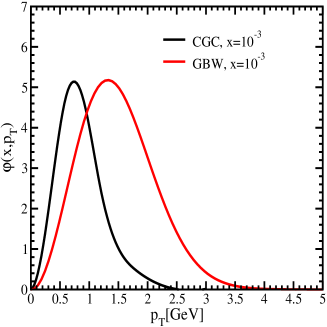
Figure 1: Function $\phi_{G}$ versus transverse momentum in different saturation models: GBW denotes the Golec-Biernat and Wusthoff model (see Ref.GBW ) while CGC denotes the model suggested in Ref.CGC . These two model have different values of the saturation momentum and the picture illustrates that $\phi(x,p_{T})$ has maximum at $p_{T}=Q_{s}$.

Having this feature of $\phi_{G}$ in mind we see that at $p_{T}\ll Q_{s}$ Eq. (1) gives

$$\frac{d\sigma}{dy\,d^{2}p_{T}}\,\,=\,\,\frac{2\pi\bar{\alpha}_{s}}{p^{2}_{\perp}}\int d^{2}k_{T}\,\,\phi^{h_{1}}_{G}\left(x_{1};\vec{k}_{T}\right)\,\phi^{h_{2}}_{G}\left(x_{2};\ \vec{k}_{T}\right)$$ (9)

One can see that at $p_{T}\to 0$ the cross section tends to infinity. Since we are talking about inclusive cross section generally speaking such situation is possible and it corresponds to increasing multiplicity of soft gluons. However, in framework of gluon saturation it looks strange. As we have discussed above, the main contribution to $\phi_{G}$ give the gluons with transverse momenta of about $Q_{s}$ while the gluons with small values of $k_{T}$ are suppressed. In other words, the correlation length between emitted gluon is of the order of $1/Q_{s}$ and we expect that emission of gluons with the wave length larger that $1/Q_{s}$ should be suppressed. Of course, soft gluons with $p_{T}\ll Q_{s}$ could be emitted in the final state but they will not propagate through the medium since the cross section is large ($\sigma T\left(b\right)\,\propto\,Q^{2}_{s}/p^{2}_{T}\gg 1$).

Figure 2: Inclusive cross section: $\vec{q}_{1}-\vec{q}_{2}=\vec{p}_{T}$.

In this letter we will show that simple formula of Eq. (1) should be changed and a new double log suppression factor ($T$) should be added. Therefore, the inclusive cross section has a form (see Fig. 2-a)

$$\frac{d\sigma}{dy\,d^{2}p_{T}}\,\,=\,\,\frac{2\pi\bar{\alpha}_{s}}{p^{2}_{\perp}}\int d^{2}q_{1}\,d^{2}q_{2}\,\delta\left(\vec{q}_{1}-\vec{q}_{2}-\vec{p}_{T}\right)\,\,\phi^{h_{1}}_{G}\left(x_{1};\vec{q}_{1}\right)\,\phi^{h_{2}}_{G}\left(x_{2};\vec{q}_{2}\right)\,T\Big{(}\frac{p^{2}_{T}}{Q^{2}_{s}}\Big{)}$$ (10)

In Eq. (10) we assume that $Q_{s,1}\approx Q_{s,2}$. The appearance of $T$ in inclusive production was found in 1980’s DDT ; PAPE ; PASR and it is related to the fact that the emission of some gluons is suppressed in the process. In our case the emission of gluons is suppressed with the value of the transverse momenta ( $p_{T,i}$) in the region: $p_{T}\,\leq\,p_{T,i}\,\leq\,Q_{s}$ (see Fig. 2-b, where the gluons which emission is suppressed, are denoted by the dashed lines). Actually, the emission of gluons with small values of $p_{T,i}$ has been taken into account in functions $\phi^{h_{i}}_{G}$ but they result in suppression of the emission for such gluons and we do not need to account separately for them.

Eq. (10) says that the emission of the gluon with $p_{T}\leq Q_{s}$ is suppressed and only gluons with $p_{t}>Q_{s}$ gives the contribution to the inclusive production. For such gluons the $k_{T}$ factorization works. This qualitative features of Eq. (10) has been confirmed by the first numerical calculculation that found the deviation from $k_{T}$ factorizxation (see Ref.BLMT ). These calculation shows that for $p_{T}<Q_{s}$ the gluon production is suppressed while for $p_{T}>Q_{s}$ the $k_{T}$ factorization works perfectly well.

We calculate the first diagrams of Fig. 2-c to illustrate the double log contribution.

This diagram is equal to

$$A\left({Fig.~{}\ref{GGT}}-c\right)\,\,=\,\,\frac{g^{3}}{(2\pi)^{4}\,i}\,\Big{(}f_{a,b^{\prime},c^{\prime}}\,f_{c^{\prime},b,a}\,f_{a^{\prime},c,c^{\prime}}\,=\,-\,\frac{N_{c}}{2}\,f_{abc}\Big{)}\,\int\,\frac{dk^{+}\,dk^{-}\,d^{2}k_{T}}{2\,q^{+}_{1}\cdot q^{-}_{2}}$$ (11)

$$\frac{q^{+}_{1,\mu}\Gamma_{\mu,\alpha,\beta}\,\Gamma_{\beta,\gamma,\nu}\,\Gamma_{\gamma,\alpha,\rho}\,q^{-}_{2,\rho}}{\left(k^{+}k^{-}\,-k^{2}_{T}\,-\,i\epsilon\right)\,\left((q^{+}_{1}-k^{+})(q^{-}_{1}-k^{-})\,-\,(\vec{q}_{1}-\vec{k})^{2}_{T}\,-\,i\epsilon\right)\,\left((q^{+}_{2}-k^{+})(q^{-}_{2}-k^{-})\,-\,(\vec{q}_{2}-\vec{k})^{2}_{T}\,-\,i\epsilon\right)}$$

In Eq. (11) we used that at high energies the propagators of gluons with momenta $q_{1}$ and $q_{2}$ can be written in the form BFKL ; GLR

$$D_{\mu^{\prime},\mu}\left(q_{1}\right)\,\,=\,\,\frac{q^{-}_{2,\mu^{\prime}}\,q^{+}_{1,\mu}}{q^{-}_{2}\,q^{+}_{1}}\,\frac{1}{q^{2}_{1,T}};\,\,\,\,\,D_{\rho,\rho^{\prime}}\left(q_{2}\right)\,\,=\,\,\frac{q^{-}_{2,\rho}\,q^{+}_{1,\rho^{\prime}}}{q^{-}_{2}\,q^{+}_{1}}\,\frac{1}{q^{2}_{2,T}};$$ (12)

In leading log(1/x) approximation we have the following kinematic constraints:

$$q^{+}_{1}\,\gg\,q^{+}_{2};\,\,\,\,q^{-}_{2}\,\gg\,q^{-}_{1};\,\,\,\,q^{+}_{1}\,q^{-}_{2}\,=\,p^{2}_{T};\,\,q^{+}_{1}\,q^{-}_{1}\,\,\ll\,\,q^{2}_{1,T};\,\,\,\,\,q^{+}_{2}\,q^{-}_{2}\,\,\ll\,\,q^{2}_{2,T};$$ (13)

Integration for $k_{T}\,>\,Q_{s}$ leads to renormalization of the coupling QCD constant. Therefore, we are interested in the kinematic region where

$$q_{i,T}\,\approx\,Q_{s}\,\gg\,k_{T}\,\gg\,p_{T}$$ (14)

Having in mind Eq. (13) and Eq. (14) we can rewrite Eq. (11) using

$$\left(q_{1}-k\right)^{2}\,\,+\,i\epsilon=\,\,(k^{-}-q^{-}_{1})\,(k^{+}-q^{+}_{1})\,\,-\,\,Q^{2}_{s}\,-\,i\epsilon;\,\,\,\left(q_{2}-k\right)^{2}\,\,+\,i\epsilon=\,\,(k^{+}-q^{-}_{2})(k^{-}-q^{-}_{2})\,\,-\,\,Q^{2}_{s}\,-\,i\epsilon;$$ (15)

One can see that for $q^{-}_{1}\,<\,k^{-}\,<\,q^{-}_{2}$ the poles in $k^{+}$ in Eq. (11) are situated in diffrent semiplanes and we can close the contour in complex plane $k^{+}$ on the pole from $\left(q_{2}-k\right)^{2}=0$. It gives

$$k^{+}_{0}\,\,=\,\,\frac{Q^{2}_{s}}{k^{-}\,-\,q^{-}_{2}}\,\,\to\,\,-\,\frac{Q^{2}_{s}}{q^{-}_{2}}$$ (16)

$$A\left({Fig.~{}\ref{GGT}}-c\right)\,\,=\,\,-\,\frac{g^{3}\pi}{(2\pi)^{3}}\,\,\frac{N_{c}}{2}\,f_{abc}\,\int\,\frac{dk^{2}_{T}\,dk^{-}}{2\,p^{2}_{T}\,q^{-}_{2}}\,\frac{q^{+}_{1,\mu}\Gamma_{\mu,\alpha,\beta}\,\Gamma_{\beta,\gamma,\nu}\,\Gamma_{\gamma,\alpha,\rho}\,q^{-}_{2,\rho}}{\left(q^{+}_{1}\,k^{-}\,+\,Q^{2}_{s}\right)\,\left(k^{-}\frac{Q^{2}_{s}}{q^{-}_{2}}\,+\,k^{2}_{T}\right)}$$ (17)

One can see that from the kinematic region given by

$$\frac{k^{2}_{T}\,q^{-}_{2}}{Q^{2}_{s}}\,\,\,\gg\,\,\,k^{-}\,\,\,\gg\,\,\,Q^{2}_{s}/q^{+}_{1};\,\,\,\,\,\,\,Q^{2}_{s}\,\,\gg\,\,k^{2}_{T}\,\,\gg\,\,p^{2}_{T}$$ (18)

we have a double log contribution, namely,

$$A\left({Fig.~{}\ref{GGT}}-c\right)\,\,=\,\,-\,\frac{g^{3}\pi}{(2\pi)^{3}}\,\,\frac{N_{c}}{2}\,f_{abc}\,\frac{1}{4\,p^{2}_{T}\,(q^{+}_{1}\,q^{-}_{2})}\,q^{+}_{1,\mu}\Gamma_{\mu,\alpha,\beta}\,\Gamma_{\beta,\gamma,\nu}\,\Gamma_{\gamma,\alpha,\rho}\,q^{-}_{2,\rho}\,\,\ln^{2}\Big{(}Q^{2}_{s}/p^{2}_{T}\Big{)}$$ (19)

Direct calculation of sum over gluon polarization in Eq. (19) leads to

$$\,\frac{1}{p^{2}_{T}}\,q^{+}_{1,\mu}\Gamma_{\mu,\alpha,\beta}\,\Gamma_{\beta,\gamma,\nu}\,\Gamma_{\gamma,\alpha,\rho}\,q^{-}_{2,\rho}\,\,=\,\,4\,(q^{+}_{1}\,q^{-}_{2})\,\Gamma_{\nu}$$ (20)

where

$$\Gamma_{\nu}\,\,=\,\,2\,\Big{(}\vec{q}_{T,1}\,\,-\,\,\frac{\vec{p}_{T}}{q^{2}_{T,1}}\Big{)}_{\nu}$$ (21)

is famous BFKL vertex BFKL .

Collecting all factors and using the notation $\Gamma^{abc}_{\nu}\,\,=\,\,2g\,f_{abc}\,\Gamma_{\nu}$ we obtain for the diagram of Fig. 2-c the following expression

$$A\left({Fig.~{}\ref{GGT}}-c\right)\,\,=\,\,-\,\frac{\bar{\alpha}_{s}}{4}\,\Gamma^{abc}_{\nu}\,\ln^{2}\Big{(}Q^{2}_{s}/p^{2}_{T}\Big{)}$$ (22)

where $\bar{\alpha}_{s}\,\,=\,\,\alpha_{s}N_{c}/\pi$. Using the well known technique (see Refs.DDT ; PAPE ) we obtain

$$T\Big{(}\frac{p^{2}_{T}}{Q^{2}_{s}}\Big{)}\,\,\,=\,\,\,\exp\Big{\{}-\frac{\bar{\alpha}_{s}}{2}\,\ln^{2}\Big{(}Q^{2}_{s}/p^{2}_{T}\Big{)}\Big{\}}$$ (23)

This result follows directly from the generalization of Low theorem for soft photonLOW for high energy scattering (Gribov’s theorem GRIB ). It says that if $p_{T}$ of emitted photon smaller than any typical transverse moneta in the process the cross section of emitted photon is equal to

$$\sigma_{\gamma}\,\,\,=\,\,\frac{\alpha}{2\pi}\,\frac{d\omega}{\omega}\,\frac{d^{2}p_{T}}{p^{2}_{T}}\,\sigma_{0}$$ (24)

where $\sigma_{0}$ is the cross section for the process without photon. This theorem has been generalized to emission of gluons (see Ref. LIPLT ). In our case the typical momentum scales of the process are $Q_{s,1}$ and $Q_{s,2}$ and, therefore, gluons with $p_{T}\,\ll\,Q_{s,1}\,\mbox{and}\,Q_{s,2}$ are emitted independently according to the Poisson distribution. The emission of one gluon will be suppressed by $\exp\left(-\langle n\rangle\right)$ where $\langle n\rangle\,=\,\frac{\bar{\alpha}_{s}}{2}\,\ln^{2}\Big{(}Q^{2}_{s}/p^{2}_{T}\Big{)}$ is the average number of emitted gluons. In the case of two different saturations scales $Q_{s,1}$ and $Q_{s,2}$ the average multiplicity $\langle n\rangle\,=\,\frac{\bar{\alpha}_{s}}{2}\,\ln^{2}\Big{(}Q^{2}_{s,min}/p^{2}_{T}\Big{)}$ where $Q_{s,min}=\mbox{min}\{Q_{s,1},Q_{s,2}\}$. For dilute-dense scattering the value of $Q_{s,min}$ vanishes and we have no additional suppression. This feature is related to the fact that the BFKL evolution has two branches one of which leads to decrease of the typical transverse momenta of gluons.

In conclusions, we would like to summarize that we suggest Eq. (10) which violates the $k_{T}$ factorization for $k_{T}<Q_{s,1}\,\mbox{and}\,Q_{s,2}$ but it is in a perfect agreement with the numerical solution for the inclusive production in Colour Glass Condensate BLMT ( see Fig. 3). We would like to emphasize that our result is based on general grounds in QCD and reflects the fact that emission of soft gluons with transverse momenta $Q_{s}\,>\,p_{i,T}\,>\,p_{T}$ has been taken into account in functions $\phi_{G}$ (see Eq. (10)) and it should not be included again in $k_{T}$-factorization formula.

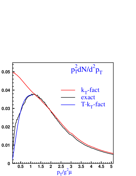
Figure 3: The single inclusive cross section $p^{2}_{T}dN/d^{2}p_{T}$ versus $p_{T}$. The low curve shows the exact solution given in Ref. BLMT . The upper curve presents the result for the inclusive cross sections from $k_{T}$-factorization. Both these curves are taken from Ref. BLMT and we are very thankful to Tuomas Lappi who shares with us the data for these curves. The blue curve (the shortest one) shows the result for Eq. (10) assuming that $\bar{\alpha}_{s}=0.1$ and $Q_{s}=1.5g^{2}\mu$.

References

(1)
S. Catani, M. Ciafaloni and F. Hautmann,
Nucl. Phys. B 366 (1991) 135.
(2)
S. Catani, M. Ciafaloni and F. Hautmann,
Nucl. Phys. Proc. Suppl. 29A (1992) 182.
(3)
J. C. Collins and R. K. Ellis,
Nucl. Phys. B 360 (1991) 3.
(4)
E. M. Levin, M. G. Ryskin, Yu. M. Shabelski and A. G. Shuvaev,
Sov. J. Nucl. Phys. 53 (1991) 657
[Yad. Fiz. 53 (1991) 1059].
(5)
L. V. Gribov, E. M. Levin and M. G. Ryskin,
Phys. Rep. 100 (1983) 1.
(6)
A. H. Mueller and J. Qiu,
Nucl. Phys. B268 (1986) 427.
(7)
L. McLerran and R. Venugopalan,
Phys. Rev. D49 (1994) 2233, 3352; D50 (1994) 2225;
D53 (1996) 458;
D59 (1999) 09400.
(8)
I. Balitsky,
[arXiv:hep-ph/9509348];
Phys. Rev.D60, 014020 (1999)
[arXiv:hep-ph/9812311]
(9)
A. H. Mueller,
Nucl. Phys. B415 (1994) 373; B437 (1995) 107.
(10)
Y. V. Kovchegov,
Phys. Rev.D60, 034008 (1999),
[arXiv:hep-ph/9901281].
(11)
J. Jalilian-Marian, A. Kovner, A. Leonidov and H. Weigert,
Phys. Rev.D59, 014014 (1999),
[arXiv:hep-ph/9706377]; Nucl. Phys.B504, 415
(1997),
[arXiv:hep-ph/9701284];
J. Jalilian-Marian, A. Kovner and H. Weigert,
Phys. Rev.D59, 014015 (1999),
[arXiv:hep-ph/9709432];
A. Kovner, J. G. Milhano and H. Weigert,
Phys. Rev.D62, 114005 (2000),
[arXiv:hep-ph/0004014] ;
E. Iancu, A. Leonidov and L. D. McLerran,
Phys. Lett.B510, 133 (2001);
[arXiv:hep-ph/0102009]; Nucl. Phys.A692, 583
(2001),
[arXiv:hep-ph/0011241];
E. Ferreiro, E. Iancu, A. Leonidov and L. McLerran,
Nucl. Phys.A703, 489 (2002),
[arXiv:hep-ph/0109115];
H. Weigert,
Nucl. Phys.A703, 823 (2002),
[arXiv:hep-ph/0004044].
(12)
D. Kharzeev, E. Levin and M. Nardi,
Nucl. Phys. A 730 (2004) 448
[Erratum-ibid. A 743 (2004) 329]
[arXiv:hep-ph/0212316]; Phys. Rev. C 71 (2005) 054903
[arXiv:hep-ph/0111315]; D. Kharzeev and E. Levin,
Phys. Lett. B 523 (2001) 79
[arXiv:nucl-th/0108006]; D. Kharzeev and M. Nardi,
Phys. Lett. B 507 (2001) 121
[arXiv:nucl-th/0012025].
(13)
D. Kharzeev, E. Levin and M. Nardi,
Nucl. Phys. A 747 (2005) 609
[arXiv:hep-ph/0408050].
(14)
Y. V. Kovchegov and K. Tuchin,
Phys. Rev. D 65 (2002) 074026
[arXiv:hep-ph/0111362].
(15)
M. A. Braun,
Eur. Phys. J. C 48 (2006) 501
[arXiv:hep-ph/0603060];
Phys. Lett. B 483 (2000), 105.
(16)
J. Jalilian-Marian and Y. V. Kovchegov,
Phys. Rev. D 70 (2004) 114017
[Erratum-ibid. D 71 (2005) 079901]
[arXiv:hep-ph/0405266].
(17)
C. Marquet,
Nucl. Phys. B 705 (2005) 319
[arXiv:hep-ph/0409023].
(18)
A. Kovner and M. Lublinsky,
JHEP 0611 (2006) 083
[arXiv:hep-ph/0609227].
(19)
E. Levin and A. Prygarin,
Phys. Rev. C 78 (2008) 065202
[arXiv:0804.4747 [hep-ph]].
(20)
A. Kormilitzin, E. Levin and A. Prygarin,
Nucl. Phys. A 813 (2008) 1
[arXiv:0807.3413 [hep-ph]].
(21)
E. Levin and K. Tuchin,
Nucl. Phys. B 573 (2000) 833
[arXiv:hep-ph/9908317].
(22)
K. J. Golec-Biernat and M. Wusthoff,
Phys. Rev. D 59 (1998) 014017
[arXiv:hep-ph/9807513]; 60 (1999) 114023
[arXiv:hep-ph/9903358].
(23)
G. Watt and H. Kowalski,
Phys. Rev. D 78 (2008) 014016
[arXiv:0712.2670 [hep-ph]];
E. Iancu, K. Itakura and S. Munier,
Phys. Lett. B 590 (2004) 199
[arXiv:hep-ph/0310338].
(24)
Y. L. Dokshitzer, D. Diakonov and S. I. Troian,
Phys. Lett. B 79 (1978) 269;
Phys. Rept. 58 (1980) 269.
(25)
G. Parisi and R. Petronzio,
Nucl. Phys. B 154 (1979) 427;
M. G. Ryskin,
Yad. Fiz. 32 (1980) 259, [Sov. ,J. Nucl. Phys.34 (1980) 133];
E. M. Levin and M. G. Ryskin,
Yad. Fiz. 32 (1980) 802, [Sov. ,J. Nucl. Phys.34 (1980) 413];
(26)
G. Pancheri-Srivastava and Y. Srivastava,
Phys. Rev. Lett. 43 (1979) 11.
(27)
E. A. Kuraev, L. N. Lipatov, and F. S. Fadin,it Sov. Phys. JETP
45 (1977) 199 ;
Ya. Ya. Balitsky and L. N. Lipatov,
Sov. J. Nucl. Phys.28 (1978) 22 .
(28)
J. P. Blaizot, T. Lappi and Y. Mehtar-Tani,
Nucl. Phys. A 846 (2010) 63
[arXiv:1005.0955 [hep-ph]].
(29)
F.E. Low, Phys. Rev. 110 (1958) 974.
(30)
V. N. Gribov,
Sov. J. Nucl. Phys. 5 (1967) 280
[Yad. Fiz. 5 (1967) 399].
(31)
L. N. Lipatov,
Nucl. Phys. B307 (1988) 705-720;
Sov. Phys. JETP 67, 1975-1981 (1988);
B. I. Ermolaev, L. N. Lipatov, V. S. Fadin,
Yad. Fiz. 45, 817-823 (1987).
(32)
W. A. Horowitz, Y. V. Kovchegov,
“Running Coupling Corrections to High Energy Inclusive Gluon Production,”
[arXiv:1009.0545 [hep-ph]].