Excitonic effects in two-dimensional massless Dirac fermions

Abstract

We study excitonic effects in two-dimensional massless Dirac fermions with Coulomb interactions by solving the ladder approximation to the Bethe-Salpeter equation. It is found that the general 4-leg vertex has a power law behavior with the exponent going from real to complex as the coupling constant is increased. This change of behavior is manifested in the antisymmetric response, which displays power law behavior at small wavevectors reminiscent of a critical state, and a change in this power law from real to complex that is accompanied by poles in the response function for finite size systems, suggesting a phase transition for strong enough interactions. The density-density response is also calculated, for which no critical behavior is found. We demonstrate that exciton correlations enhance the cusp in the irreducible polarizability at $2k_{F}$, leading to a strong increase in the amplitude of Friedel oscillations around a charged impurity.

I INTRODUCTION

Graphene is a two-dimensional honeycomb lattice of carbon atoms. Near zero doping, the low energy quasiparticle states are well-described by two-dimensional massless Dirac fermions (MDF’s). Graphene supports two species of these, centered at the two inequivalent corners of the Brillouin zone. At low or zero doping, the properties of graphene are in many ways quite different than those of a doped semiconductor, in large part because of the unusual properties of MDF’s Neto et al. (2009); Das .

One interesting class of questions about graphene involve Coulomb interactions. In a seminal study, Gonzalez, Guinea and Vozmediano Gonzalez et al. (1994) demonstrated that weak Coulomb interactions in undoped graphene are marginally irrelevant, invalidating the basic premise of strong screening that underlies the standard treatment of an electron gas as a weakly interacting Fermi liquid. Moreover, simple estimates of the strength of Coulomb interactions, characterized by an effective fine structure constant $\beta=e^{2}/\epsilon\hbar v_{F}$, where $v_{F}$ is the speed of electrons near a Dirac point and $\epsilon$ is the effective dielectric constant due to a substrate upon which the graphene may be adsorbed, suggest that Coulomb interactions are effectively large ($\beta>1$) if $\epsilon\sim 1$. This suggests that properties of graphene near zero doping should be rather different than those of non-interacting MDF’s; for example, a gap may open in the quasiparticle spectrum dru , so that rather than behaving as a metal the system would be insulating. In real experiments there is little evidence for such dramatic effects of interactions, most likely because disorder effects overwhelm those of Coulomb interactions Das . If so, one may suppose that interaction effects could become apparent if sufficiently clean graphene samples can be created. In this work, we study this theoretical clean limit, and focus on unusual properties which can emerge in linear response functions for two-dimensional MDF’s due to Coulomb interactions. As we shall see, these have important consequences for the induced charge distribution around an impurity, and suggest that the MDF description breaks down even before a gap opens in the spectrum.

The unusual effects of a Coulomb potential for MDF’s are already apparent in their response to a Coulomb charge $Ze$, even when there are no interactions among the electrons themselves. The wavefunctions for this problem are essentially exactly calculable shy ; per (a); bis ; ter ; per (b); kot . One finds that the $m$-th circular component of an electron wavefunction has the short distance form $\psi_{m}(r)\sim r^{\sqrt{(m+1/2)^{2}-Z^{2}\beta^{2}}-1/2}$ at a distance $r$ from the impurity. This is an unusual situation in that the exponent is a function of the impurity charge, so that the wavefunctions have a non-analytic dependence on the potential strength at short distances. This cannot be reproduced at any finite order in perturbation theory. When $Z\beta$ is above a critical value, the short distance exponent becomes complex, corresponding to a maximal penetration of the centrifugal barrier (the effective potential due to the angular momentum in the radial equation for the wavefunction) by the electrons. We refer to this phenomenon as “Coulomb implosion”, and it is analogous shy to the breakdown of the vacuum in the vicinity of a highly charged nucleus in QED Schwabl (2008). In graphene, this breakdown is accompanied by the formation of a charge cloud around the impurity with density falling off as $1/r^{2}$, which is absent for $Z\beta$ below its critical value. The propagation of a short distance effect (penetration of the centrifugal barrier) to long distances (appearance of the charge cloud) is one of the special properties of MDF’s, and it reflects the absence of any length scale in the Dirac equation itself. As we shall see, there are many-body analogs of these phenomenon which become apparent in some of the linear response functions.

To address the many-body problem, it is preferable to assess the non-analytic content of a linear response function as a function of momentum rather than position. To see how this might be done, we revisit the problem of non-interacting MDF’s in the presence of a Coulomb impurity, and analyze how the short distance behavior described above is manifested in a momentum representation. Not surprisingly, we find that the scattering wavefunctions, when expressed in a momentum representation, display power law behavior at large momentum, with an exponent that changes from real to complex for $Z\beta$ exceeding the same critical value found in the real space analysis. The momentum space analysis in terms of scattering states naturally suggests that one might find similar behavior in vertex functions evaluated in the ladder approximation fet . Ladder diagrams play an important role in interacting systems because they allow one to incorporate excitonic correlations in virtual particle-hole pairs that are generated by the interaction. We analyze this approximation for a generic four-point vertex function of MDF’s with Coulomb interactions, and find both the non-analytic power law behavior at large momentum and a change from real to complex exponent, in this case when $\beta$ exceeds some critical value. The analysis suggests the system undergoes a quantum phase transition at this critical value, since the exponent necessarily behaves in a non-analytic way as a function of the parameter $\beta$. Interestingly, we shall see that the equations for the vertex function suggest that this transition is infinite order, suggesting the transition may be in the same universality class as classical two dimensional systems undergoing a Kosterlitz-Thouless (KT) transition Nelson (2002).

To relate the four point vertex function to measurable quantities, we use it to form three-point vertex functions which can then be used to directly compute linear response functions. Two are of particular interest. The density response function (equivalently, the density-density correlation function) expresses the screening response of the system to an external potential, including due to impurities or inhomogeneities in the system. We find that the non-analyticity of the four-leg vertex does not present itself in this particular quantity. Nevertheless, we demonstrate that exciton effects, as expressed in the ladder diagrams, have important quantitative effects for for doped systems, where we find a strong enhancement of Friedel oscillations around a charged impurity relative to the non-interacting case.

The other important response function involves the charge imbalance between the two sublattices, the antisymmetric response function. (Some results on this were reported by us previously Wang et al. (2010).) Here we indeed find non-analytic behavior analogous to the Coulomb impurity problem for non-interacting MDF’s. Although this non-analyticity is apparent at large wavevectors in the four-leg vertex, the absence of length scale in the problem leads to power law behavior emerging at small wavevectors in the response function. In particular this applies to an impurity placed asymmetrically with respect to the graphene sublattices, which is known to induce very different charge responses on them Cheianov and Falko (2006); Brey et al. (2007); Wehling et al. (2007); Yazyev and Helm (2007). The sublattice-antisymmetric component of this acquires a power law tail, with exponent that changes from real to complex above a critical value of $\beta$. Interestingly, when a finite size cutoff is included in the calculation, we find poles in the response function, suggesting a quantum phase transition to a state with different charge densities on the sublattices, and hence a state with spontaneously broken chiral symmetry Khveshchenko (2001); Gor . These poles however merge together into a branch cut in the thermodynamic limit Wang et al. (2010), suggesting a state fluctuating among ones with the chiral symmetry broken in different possible ways, and no mean-field mass gap. This may represent a phase transition that is a precursor to one in which a real gap develops in the spectrum dru .

This article is organized as follows. We begin with a study of the single impurity problem in the momentum representation in Section II and identify the signatures for the short-distance power law behavior and Coulomb implosion. With this simpler example to guide us, in Section III we study the ladder approximation to the Bethe-Salpeter equation for the 4-leg vertex. This approximation is the many-body analog of the Lippmann-Schwinger equation studied in Section II. We show that the vertex function has a power law behavior in momentum, and the exponent changes from real to complex above a certain value of coupling constant $\beta$. The interesting properties of the antisymmetric response are discussed in Section IV. Finally, in Section V we focus on the density-density response function in the ladder approximation, and demonstrate the important quantitative effects caused by excitonic correlations.

II Impurity problem in the momentum representation

We begin by discussing the problem of MDF’s in the presence of a Coulomb impurity in terms of scattering states. The standard (Lippmann-Schwinger) equation for scattering states Merzbacher (1970) takes the form

$$\psi^{(+)}(\vec{x})=\psi^{(0)}(\vec{x})+\int d^{2}\vec{y}G^{\text{DE}}(\vec{x}-\vec{y})V(\vec{y})\psi^{(+)}(\vec{y}),$$ (1)

where $G^{\text{DE}}$ is the (matrix) Green’s function determined by the differential equation (DE) $(-\hbar v_{F}\vec{\sigma}\cdot\hat{p}+\varepsilon\openone)G^{\text{DE}}(\vec{x})=\delta^{(2)}(\vec{x})$, $V(\vec{y})=Ze^{2}/\epsilon|\vec{y}|$ is the impurity potential and $\psi^{(0)}$ is an eigenstate for $V=0$. Fourier transforming Eq. (1), we have

$$\psi^{(+)}(\vec{p})=\psi^{(0)}(\vec{p})+G^{\text{DE}}(\vec{p})\int\frac{d^{2}p^{\prime}}{(2\pi)^{2}}V(\vec{p}-\vec{p}\,^{\prime})\psi^{(+)}(\vec{p}\,^{\prime}).$$ (2)

It is convenient to express the Lippmann-Schwinger equation in terms of angular momentum states. Introducing the angular components

$$\psi_{m}(p) =\int^{2\pi}_{0}\frac{d\theta_{p}}{2\pi}e^{-im\theta_{p}}\psi(\vec{p}),$$ (3)

$$V(|\vec{p}-\vec{p}\,^{\prime}|) =-Ze^{2}\sum_{n}e^{-in(\theta_{\vec{p}}-\theta_{\vec{p}\,^{\prime}})}f_{n}(p/p^{\prime})/p^{\prime},$$ (4)

$$f_{n}(x) =\int^{2\pi}_{0}\frac{d\theta}{2\pi}\frac{e^{-in\theta}}{[1+x^{2}-2x\cos(\theta)]^{1/2}},$$ (5)

where $\theta_{\vec{p}}$ is the angle between the vector $\vec{p}$ and the $\hat{x}$ axis, and using

$$G^{\text{DE}}(\vec{p})=\frac{1}{\varepsilon^{2}-(\hbar v_{F}p^{2})}[\varepsilon\openone+\hbar v_{F}(p_{x}\sigma^{x}+p_{y}\sigma^{y})],$$ (6)

where $\sigma^{x}$ and $\sigma^{y}$ are the Pauli matrices, Eq. (2) may be written in the form

$$\psi^{(+)}_{1,m} = \psi^{(0)}_{1,m}(p)$$

$$-\frac{Ze^{2}p}{\varepsilon^{2}-(\hbar v_{F}p)^{2}}[\varepsilon\int^{\infty}_{0}xf_{-m}(x)\psi^{(+)}_{1,m}(xp)dx$$

$$+\hbar v_{F}p\int^{\infty}_{0}xf_{-(m+1)}(x)\psi^{(+)}_{2,m+1}(xp)dx],$$

$$\psi^{(+)}_{2,m+1} = \psi^{(0)}_{2,m+1}(p)$$

$$-\frac{Ze^{2}p}{\varepsilon^{2}-(\hbar v_{F}p)^{2}}[\hbar v_{F}p\int^{\infty}_{0}xf_{-m}(x)\psi^{(+)}_{1,m}(xp)dx$$

$$+\varepsilon\int^{\infty}_{0}xf_{-(m+1)}(x)\psi^{(+)}_{2,m+1}(xp)dx].$$

Motivated by the observation that power law behavior emerges in the wavefunctions at small distances, we search for power law solutions at large wavevector. Using the ansatz

$$\psi^{(+)}_{\alpha,m}(p)=\frac{c_{\alpha,m}}{p^{s}}\mbox{ for $p\rightarrow\infty$},$$ (9)

and neglecting terms of lower order of $p$, Eqs. II may be written as

$$\left(\begin{array}[]{cc}1&-Z\beta I_{m+1}(s)\\ Z\beta I_{m}(s)&-1\\ \end{array}\right)\left(\begin{array}[]{c}c_{1,m}\\ c_{2,m+1}\\ \end{array}\right)=0$$ (14)

where

$$I_{m}(s)=\int^{\infty}_{0}x^{1-s}f_{-m}(x)dx.$$ (15)

Eqs. 14 will have non-vanishing solutions provided

$$1-(Z\beta)^{2}I_{m}(s)I_{m+1}(s)=0.$$ (16)

One may easily show that $I_{m}(s)$ has a minimum at $s=3/2$ for any integer $m$, so for $Z\beta$ larger than a critical $(Z\beta)_{c}$, the solution $s$ to Eq. 16 becomes complex. For $m=0$, $(Z\beta)_{c}=1/2$; for $m=1$, $(Z\beta)_{c}=3/2$, etc. This change of behavior corresponds to that found in the real space analysis of the Coulomb impurity problem shy . For $Z\beta>(Z\beta)_{c}$ (for a given $m$), the complex values of $s$ cause $\psi^{(+)}_{\alpha,m}(p)$ to oscillate at small $r$, with no well-defined value of $\psi^{(+)}_{\alpha,m}(r)$ as $r\rightarrow 0$. This leads to an ill-defined problem unless a boundary condition for small but finite $r$ is imposed shy . This suggests that some quantities are sensitive to the short scale cutoff in the problem, a behavior which we will see holds true as well for some response response functions when Coulomb interactions are included. Using the above analysis as a guide, we now turn to this more complicated problem.

III General 4-leg vertex

As we saw in the last section, the signature of Coulomb implosion in the momentum representation is that the exponent of the power law of the wavefunction becomes complex. The basic physics in Eq. (1) is clear: in a perturbative expansion in $V$, the electron can be scattered arbitrarily many times by the impurity, and the non-analytic, power law behavior emerges from a superposition of all these possibilities. If we substitute the electron-impurity scattering with electron-hole scattering due to Coulomb interactions, we may expect a many-body analog of both the power law behavior and of Coulomb implosion. The signature of these should be contained in the general 4-leg vertex function in the electron-hole channel.

To compute this, we note fet that the ladder approximation to the 4-leg vertex (Fig. 1) has the same structure of multiple scattering of an electron from a hole as does an expansion of Eq. 1 in powers of $V$. The Bethe-Salpeter equation resulting from this ladder sum has the form fet

$$\Gamma_{\alpha\beta,\gamma\delta}(p_{1},p_{2};p_{3},p_{4})=U(p_{1}-p_{3})\delta_{\alpha\gamma}\delta_{\beta\delta}$$

$$+\frac{i}{\hbar}\int\frac{d^{3}q}{(2\pi)^{3}}U(q)G^{(0)}_{\alpha\mu}(p_{1}-q)G^{(0)}_{\nu\beta}(p_{2}-q)\Gamma_{\mu\nu,\gamma\delta}(q),$$

where $\Gamma$ is the vertex function whose arguments are three momenta [spatial components (momentum) $\vec{p}$ and time component (frequency) $p_{0}$ ], $U(p)=2\pi e^{2}/\epsilon|\vec{p}|$ is the Coulomb interaction, and

$$G^{(0)}(p_{0},\vec{p})=$$

$$\frac{p_{0}+\mu/\hbar+v_{F}\vec{p}\cdot\vec{\sigma}}{(p_{0}+\mu/\hbar)^{2}-(v_{F}\vec{p})^{2}+i\delta\cdot\text{sgn}(p_{0})(p_{0}+\mu/\hbar)}$$

is the time-ordered Green’s function for non-interacting Dirac fermions, and we have allowed the possibility of a non-zero chemical potential $\mu$.

Figure 1: Ladder approximation to the Bethe-Salpeter equation.

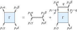
Following Ref. fet, , we introduce two new functions $Q$ and $\chi$ via the relations

$$\Gamma_{\alpha\beta,\gamma\delta}(p_{1},p_{2};p_{3},p_{4})=$$

$$\int\frac{d^{3}q}{(2\pi)^{3}}U(q)Q_{\alpha\beta,\gamma\delta}(p_{1}-q,p_{2}-q;p_{3},p_{4}),$$

$$\chi_{\alpha\beta,\gamma\delta}(\vec{p},\vec{p}\,^{\prime};P)=$$

$$\int\frac{dp_{0}}{2\pi}Q_{\alpha\beta,\gamma\delta}(p+\frac{1}{2}P,p-\frac{1}{2}P;p^{\prime}+\frac{1}{2}P,p^{\prime}-\frac{1}{2}P).$$

In these expressions, $P$ represents the four-momentum of the particle-hole pair, which may be understood as entering the vertex at the bottom of the diagrams in Fig. 1 and exiting at the top. In this interpretation, $p$ then represents the relative momentum of the pair before the collision, and $p^{\prime}$ the momentum afterwards. These equations allow Eq. (III) to take the form

$$\chi_{\alpha\beta,\gamma\delta}(\vec{p},\vec{p}\,^{\prime};\vec{P})=\delta_{\alpha\gamma}\delta_{\beta\delta}(2\pi)^{2}\delta^{(2)}(\vec{p}\,^{\prime}-\vec{p})$$

$$+K_{\alpha\beta,\mu\nu}(\vec{p},\vec{P})\int\frac{d^{2}q}{(2\pi)^{2}}U(\vec{q})\chi_{\mu\nu,\gamma\delta}(\vec{p}-\vec{q},\vec{p}\,^{\prime};\vec{P}),$$

where

$$K_{\alpha\beta,\mu\nu}(\vec{p},\vec{P})\equiv\frac{i}{\hbar}\int\frac{dp_{0}}{2\pi}G^{(0)}_{\alpha\mu}(p+\frac{1}{2}P)G^{(0)}_{\nu\beta}(p-\frac{1}{2}P).$$ (22)

Note that because we have integrated over $p_{0}$, there is no frequency dependence in $K$ or $\chi$ fet . The quantity $\chi$ can be used to directly to construct static response functions, as we shall see below.

In the case of the Dirac particle colliding with a Coulomb impurity we found power law behavior for large momenta, specifically from collisions involving a large change in momentum ($|\vec{p}|>>|\vec{p}^{\prime}|$ in Eq. 2.) Since in the two-body problem, the particle and hole scatter from one another, we search for analogous behavior in the vertex functions at large momentum difference $|\vec{p}-\vec{p}\,^{\prime}|$. For example, for fixed $P$ and $\vec{p}\,^{\prime}$, when $|\vec{p}\,|\rightarrow\infty$, the equations for $\chi_{11,\gamma\delta}$ and $\chi_{22,\gamma\delta}$ become

$$\chi_{11,\gamma\delta}(\vec{p}\,)=$$

$$\frac{1}{4\hbar v_{F}|\vec{p}\,|}\int\frac{d^{2}q}{(2\pi)^{2}}U(\vec{p}-\vec{q})[\chi_{11,\gamma\delta}(\vec{q})-\chi_{22,\gamma\delta}(\vec{q})],$$

$$\chi_{22,\gamma\delta}(\vec{p}\,)=$$

$$\frac{1}{4\hbar v_{F}|\vec{p}\,|}\int\frac{d^{2}q}{(2\pi)^{2}}U(\vec{p}-\vec{q})[-\chi_{11,\gamma\delta}(\vec{q})+\chi_{22,\gamma\delta}(\vec{q})].$$

Note in these expressions terms of order $P/p$, $p\,^{\prime}/p$ have been dropped, and $\vec{p}$ and $P$ are suppressed in the arguments of $\chi$.

Introducing circular moments as before, i.e.

$$\chi^{(m)}=\int^{2\pi}_{0}\frac{d\theta_{p}}{2\pi}e^{-im\theta_{p}}\chi(\vec{p}),$$ (25)

and using the ansatz

$$\chi^{(m)}_{11,\gamma\delta}(p) =\frac{C^{(m)}_{11,\gamma\delta}}{p^{s}},$$ (26)

$$\chi^{(m)}_{22,\gamma\delta}(p) =\frac{C^{(m)}_{22,\gamma\delta}}{p^{s}},$$ (27)

the $m$-th angular component of the above coupled equations reduces to

$$\left(\begin{array}[]{c c}\frac{4}{\beta}-I_{m}(s)&I_{m}(s)\\ I_{m}(s)&\frac{4}{\beta}-I_{m}(s)\end{array}\right)\left(\begin{array}[]{c}C^{(m)}_{11,\gamma\delta}\\ C^{(m)}_{22,\gamma\delta}\end{array}\right)=0.$$ (32)

Nontrivial solutions to this set of homogeneous linear equations may be found if

$$2/\beta=I_{m}(s),$$ (33)

which determines the exponent $s$ for a given $\beta$. The critical $\beta$ where the exponent of the power law becomes complex is $\beta_{c}=2/I_{m}(3/2)$. We thus see the many-body problem has a Coulomb implosion instability analogous to what is found in the Coulomb impurity problem for non-interacting MDF’s. A natural interpretation for this instability is that it indicates a transition to a gapped, excitonic insulator state Gor ; Khveshchenko (2001). However, as we shall see below, when analyzed in terms of the appropriate linear response function, such an interpretation is only consistent when considering a finite size system Wang et al. (2010); in the thermodynamic limit the transition is likely to a state with a fluctuating mass gap.

$\chi^{(m)}_{11,\gamma\delta}$ and $\chi^{(m)}_{22,\gamma\delta}$ are not the only components of the vertex function which display instabilities. An analogous instability appears for $\chi_{12,\gamma\delta}$ and $\chi_{21,\gamma\delta}$, which are governed by the equations

$$\chi_{12,\gamma\delta}(\vec{p})=$$

$$\frac{1}{4\hbar v_{F}|\vec{p}|}\int\frac{d^{2}q}{(2\pi)^{2}}U(\vec{p}-\vec{q})[\chi_{12,\gamma\delta}(\vec{q})-e^{-2i\theta_{\vec{p}}}\chi_{21,\gamma\delta}(\vec{q})],$$

$$\chi_{21,\gamma\delta}(\vec{p})=$$

$$\frac{1}{4\hbar v_{F}|\vec{p}|}\int\frac{d^{2}q}{(2\pi)^{2}}U(\vec{p}-\vec{q})[-e^{2i\theta_{\vec{p}}}\chi_{12,\gamma\delta}(\vec{q})+\chi_{21,\gamma\delta}(\vec{q})].$$

The equations for the coefficients in the power law ansatz are

$$\left(\begin{array}[]{c c}\frac{4}{\beta}-I_{m}(s)&I_{m+2}(s)\\ I_{m}(s)&\frac{4}{\beta}-I_{m+2}(s)\end{array}\right)\left(\begin{array}[]{c}C^{(m)}_{12,\gamma\delta}\\ C^{(m+2)}_{21,\gamma\delta}\end{array}\right)=0,$$ (40)

so that the equation for $s$ is

$$4/\beta=I_{m}(s)+I_{m+2}(s).$$ (41)

The critical $\beta$ for the 12 and 21 components of $\chi$ is $\beta_{c}^{\prime}=4/[I_{m}(3/2)+I_{m+2}(3/2)]>\beta_{c}$. This suggests that $\chi^{(m)}_{11,\gamma\delta}$ and $\chi^{(m)}_{22,\gamma\delta}$ can develop complex exponents before $\chi^{(m)}_{12,\gamma\delta}$ and $\chi^{(m)}_{21,\gamma\delta}$ as $\beta$ is increased from small values. We will see more generally that certain combinations of the vertex functions do not appear to develop power law behavior at all; most importantly this appears to be the case for the vertex function relevant to the density-density response function. In this context, we note that the coefficients satisfy the conditions $C^{(m)}_{11,\gamma\delta}=-C^{(m)}_{22,\gamma\delta}$ and $C^{(m)}_{12,\gamma\delta}=-C^{(m+2)}_{21,\gamma\delta}$, so that $\chi_{11,\gamma\delta}(\vec{p})=-\chi_{22,\gamma\delta}(\vec{p})$ and $\chi_{12,\gamma\delta}(\vec{p})=-\chi_{21,\gamma\delta}(\vec{p})$. These relations among the components of $\chi_{\alpha\beta,\gamma\delta}$ can also be seen from Eqs. III and 22 when expressed in terms of circular moments. The density-density response turns out to involve $\chi_{\alpha\alpha,\gamma\gamma}$ (repeated indices here are summed), so that the power law behavior is canceled away.

We have verified our analysis by numerically solving the Bethe-Salpeter equation in the form of Eq. (III). We use polar coordinates for the integration and change each dimension of the integration to a discrete sum, independent of the other dimension, i.e.

$$\int^{2\pi}_{0}d\theta\int^{\Lambda}_{0}dqf(\theta,q)\rightarrow\sum_{i=1}^{N_{\theta}}w_{i}\sum_{j=1}^{N_{q}}w_{j}f(\theta_{i},q_{j}),$$ (42)

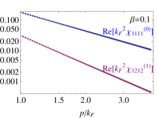
where $\Lambda$ is the momentum cutoff and $f$ denotes a general integrand, and the discretization in each dimension is done according to the Gauss-Legendre rule Num . Now the integral equation is changed to a set of linear equations and can be solved using any existing subroutine, e.g. the appropriate routine in the Lapack package. Some examples of our results are shown in Fig. 2. As can be seen, the vertex functions follow power law forms, and the exponents are close to those expected from our asymptotic analysis, both below and above the critical value of $\beta$.

An interesting aspect of these results is that the change of the exponent $s=s^{\prime}+is^{\prime\prime}$ from real to complex at a finite value of $\beta$ (i.e., $s^{\prime\prime}$ is zero for $\beta<\beta_{c}$ but is non-vanishing for $\beta>\beta_{c}$) suggests that quantities calculated from it will have a non-analyticity at $\beta_{c}$. However, any such singularity must be of infinite order. For example, if there is a cusp in $\chi$ at $\beta=\beta_{c}$, then there would be a contribution of the form $B_{\alpha\beta,\gamma\delta}(\vec{p},\vec{p}\,^{\prime};P)\delta(\beta-\beta_{c})$ in $\partial^{2}\chi/\partial\beta^{2}$. Differentiating Eq. (III) with respect to $\beta$ twice, and requiring that the coefficients of $\delta(\beta-\beta_{c})$ on both sides of the equation are the same, we find an equation for $B$,

$$B_{\alpha\beta,\gamma\delta}(\vec{p},\vec{p}\,^{\prime};P)=$$

$$+K_{\alpha\beta,\mu\nu}(\vec{p},\vec{P})\int\frac{d^{2}q}{(2\pi)^{2}}\left[U(\vec{q})|_{\beta=\beta_{c}}\right]B_{\mu\nu,\gamma\delta}(\vec{p}-\vec{q},\vec{p}\,^{\prime};P).$$

This is nothing but a homogeneous version of Eq. (III), with $\beta$ [in $U(\vec{q})$] set to $\beta_{c}$. If Eq. (III) has a non-vanishing solution, then Eq. (III) would also have a contribution from such a solution, and we would expect $\chi$ to be divergent at $\beta=\beta_{c}$. Our explicit solutions, both in the asymptotic and the numerical analysis, show that this is not the case, so that no cusp can be present. Similarly, higher order derivatives of $\chi$ also cannot have cusps. It follows that the singular behavior at $\beta=\beta_{c}$ – and any phase transition it may represent – is of infinite order, a property it shares with KT transitions Nelson (2002). In our analysis of the antisymmetric response below we shall see further hints of a connection to the KT universality class in this system.

Figure 2: (Color online) Some examples of power laws from solving Eq. (III) numerically. $P=0$ and $p\,^{\prime}=k_{F}/2$. (a) $\beta=0.1<\beta_{c}$, the solid lines are fits with the model $C/\tilde{p}^{s}$, where $\tilde{p}\equiv p/k_{F}$. For $\Re\chi^{(0)}_{1111}$ we get $s=2.02$ from fitting, $s=1.95$ from solving Eq. (33). For $\Re\chi^{(1)}_{1212}$ we get $s=3.09$ from fitting, $s=3.05$ from solving Eq. (41). (b) $\beta=1>\beta_{c}$. The solid line is a fit with $C\cos\left(s^{\prime\prime}\log\tilde{p}+\delta\right)/\tilde{p}^{s^{\prime}}$. The fitting gives $s^{\prime}=1.57$ and $s^{\prime\prime}=0.78$, while Eq. (33) gives $s^{\prime}=1.5$, $s^{\prime\prime}=0.60$.

The symmetries of the components of $\chi$ discussed above led to a cancellation of the power law behavior in the density-density response function. This same symmetry suggests that in a response function of the form $\sigma^{z}_{\alpha\beta}\chi_{\alpha\beta,\gamma\delta}$, with $\sigma^{z}$ the Pauli matrix, the power law should be retained. This represents the response of the density difference between the $A$ and $B$ sublattices due to a potential that is antisymmetric in sublattice index. Any potential that breaks sublattice symmetry will have a component of this antisymmetric response, so that it is in principle physically accessible. As we shall show next, the antisymmetric response does capture the power law as well as the Coulomb implosion physics.

IV antisymmetric response

We define the antisymmetric response as

$$M(\vec{q})=-\frac{i}{A}\int^{\infty}_{0}dt\left<[\hat{m}_{z}(-\vec{q},t),\hat{m}_{z}(\vec{q},0)]\right>,$$ (44)

$$\hat{m}_{z}(\vec{q})=\sigma^{z}_{\alpha\beta}\hat{\rho}_{\alpha\beta}(\vec{q}),\mbox{ }\hat{\rho}_{\alpha\beta}\equiv\sum_{\vec{k}}a^{\dagger}_{\vec{k}+\vec{q},\alpha}a_{\vec{k},\beta},$$ (45)

where $A$ is the area of the sample, repeated indices are summed, and henceforward we will set $\hbar=1$. In principle $M(\vec{q})$ can be determined experimentally by measuring the screening charge induced by an impurity placed asymmetrically with respect to the two sublattices, i.e. anywhere except in the center of a hexagon, or at the middle point of a carbon-carbon bond. The difference between densities on the two sublattices $\hat{m}_{z}$ is an interesting operator because when $<\hat{m}_{z}(\vec{q})>$ is non-vanishing, there is a dynamically generated Dirac mass Khveshchenko (2001); Gor .

Figure 3: (Color online) (a) Diagrammatical equation for the 3-leg vertex $\tilde{\Gamma}^{M}_{\alpha\beta}(\vec{k},\vec{q})$ with $\sigma^{z}$ as the zeroth order vertex (the shaded cross in the figure). (b) Diagram for $M(\vec{q})$.

IV.1 Diagrammatic Expansion and Ladder Approximation

The diagrammatic representation for $M(\vec{q})$ is illustrated in Fig. 3, along with the summation of ladder diagrams, Fig. 3, representing our approximation for the vertex function. Notice there are no bubble diagrams in the diagrammatic expansion of $M(\vec{q})$; there are only irreducible diagrams. Reducible diagrams for this quantity turn out to vanish, as we now show. Any reducible diagram will have at its end an insertion of the form illustrated in Fig. 4, in which there is a Coulomb vertex $\tilde{\Gamma}$. This insertion represents a multiplicative contribution to the diagram of the form

$$i\int\frac{d^{3}k}{(2\pi)^{3}}\sigma^{z}_{\alpha_{1}\beta_{1}}G^{(0)}_{\alpha_{2}\alpha_{1}}(k+q)G^{(0)}_{\beta_{1}\beta_{2}}(k)\tilde{\Gamma}_{\alpha_{2}\beta_{2}}(\vec{k},q)$$ (46)

$$\equiv\int\frac{d^{2}k}{(2\pi)^{2}}\sigma^{z}_{\alpha_{1}\beta_{1}}\tilde{K}_{\alpha_{1}\beta_{1}\alpha_{2}\beta_{2}}(\vec{k},\vec{q})\tilde{\Gamma}_{\alpha_{2}\beta_{2}}(\vec{k},\vec{q})$$

$$\equiv\int\frac{d^{2}k}{(2\pi)^{2}}\sigma^{z}_{\alpha_{1}\beta_{1}}\tilde{\chi}_{\alpha_{1}\beta_{1}}(\vec{k},\vec{q})$$

In these expressions the overhead tilde denotes quantities pertaining to 3-leg vertex. Note also that we have set $q_{0}=0$ in the second line. Assuming the Coulomb vertex is given by a ladder sum, the equation determining $\tilde{\chi}$ is [Fig. 4]

$$\tilde{\Gamma}_{\alpha_{2}\beta_{2}}({\vec{k}},{\vec{q}})=\delta_{\alpha_{2}\beta_{2}}+$$

$$\int\frac{d^{2}q^{\prime}}{(2\pi)^{2}}U(|\vec{q^{\prime}}|)\tilde{K}_{\alpha_{2}\beta_{2}\gamma_{1}\gamma_{2}}(\vec{k}-\vec{q}^{\prime},\vec{q})\tilde{\Gamma}_{\gamma_{1}\gamma_{2}}(\vec{k}-\vec{q}^{\prime},\vec{q}),$$

so that $\tilde{\chi}$ satisfies

$$\tilde{\chi}_{\alpha\beta}(\vec{k},\vec{q})=\tilde{K}_{\alpha\beta\alpha_{2}\alpha_{2}}(\vec{k},\vec{q})$$

$$+\tilde{K}_{\alpha\beta\alpha_{2}\beta_{2}}(\vec{k},\vec{q})\int\frac{d^{2}q^{\prime}}{(2\pi)^{2}}U(|\vec{q}^{\prime}|)\tilde{\chi}_{\alpha_{2}\beta_{2}}(\vec{k}-\vec{q}^{\prime},\vec{q}).$$

Figure 4: (Color online) (a) An insertion for the reducible diagram for $M(\vec{q})$. (b) The diagram equation for the 3-leg Coulomb vertex $\tilde{\Gamma}_{\alpha_{2}\beta_{2}}(\vec{k},q)$.

More explicitly, the 11 and 22 components of Eq. IV.1, in the undoped case ($\mu=0$), are

$$\tilde{\chi}_{11}(\vec{k},\vec{q})=\frac{1-e^{-i(\theta_{k}-\theta_{+})}}{2(k+|\vec{k}+\vec{q}|)}+\frac{1}{2(k+|\vec{k}+\vec{q}|)}$$

$$\int\frac{d^{2}k^{\prime}}{(2\pi)^{2}}U(\vec{k}-\vec{k}^{\prime})\left[\tilde{\chi}_{11}(\vec{k}^{\prime},\vec{q})-e^{-i(\theta_{k}-\theta_{+})}\tilde{\chi}_{22}(\vec{k}^{\prime},\vec{q})\right],$$

$$\tilde{\chi}_{22}(\vec{k},\vec{q})=\frac{1-e^{i(\theta_{k}-\theta_{+})}}{2(k+|\vec{k}+\vec{q}|)}+\frac{1}{2(k+|\vec{k}+\vec{q}|)}$$

$$\int\frac{d^{2}q^{\prime}}{(2\pi)^{2}}U(\vec{k}-\vec{k}^{\prime})\left[-e^{i(\theta_{k}-\theta_{+})}\tilde{\chi}_{11}(\vec{k}^{\prime},\vec{q})+\tilde{\chi}_{22}(\vec{k}^{\prime},\vec{q})\right],$$

where $\theta_{k}$ and $\theta_{+}$ are the angular coordinates of the two-dimensional momenta $\vec{k}$ and $\vec{k}+\vec{q}$ respectively. Without loss of generality, we can set $q_{y}=0$, from which it is easy to see that $\tilde{\chi}_{22}(k_{x},-k_{y};\vec{q})=\tilde{\chi}_{11}(k_{x},k_{y};\vec{q})$. When this is substituted into the last of Eqs. 46 one readily sees that this insertion vanishes. Thus our approximation for $M(\vec{q})$ includes only the irreducible ladder diagrams.

The calculation of the $M(\vec{q})$ follows steps very analogous to those described for the 4-leg vertex, and were outlined in Ref. Wang et al., 2010. The equation for the 3-leg antisymmetric vertex [Fig. 3] is

$$\tilde{\Gamma}^{M}_{\alpha\beta}({\vec{k}},{\vec{q}})= \,\sigma^{z}_{\alpha\beta}+\int\frac{d^{2}q^{\prime}}{(2\pi)^{2}}U(|\vec{q^{\prime}}|)\tilde{K}_{\alpha\beta\gamma\delta}(\vec{k}-\vec{q}^{\prime},\vec{q})$$

$$\times\tilde{\Gamma}^{M}_{\gamma\delta}(\vec{k}-\vec{q}^{\prime},\vec{q}).$$ (51)

Defining $\tilde{\chi}^{M}_{\alpha\beta}(\vec{k},\vec{q})=\tilde{K}_{\alpha\beta\gamma\delta}(\vec{k},\vec{q})\tilde{\Gamma}^{M}_{\gamma\delta}(\vec{k},\vec{q}),$ one finds

$$\tilde{\chi}^{M}_{\alpha\beta}(\vec{k},\vec{q})= \,\tilde{K}_{\alpha\beta\gamma\delta}(\vec{k},\vec{q})\sigma^{z}_{\gamma\delta}+\tilde{K}_{\alpha\beta\gamma\delta}(\vec{k},\vec{q})$$

$$\times\int\frac{d^{2}q^{\prime}}{(2\pi)^{2}}U(|\vec{q}^{\prime}|)\tilde{\chi}^{M}_{\gamma\delta}(\vec{k}-\vec{q}^{\prime},\vec{q}).$$ (52)

This quantity is related to the susceptibility by

$$M(\vec{q})=\int\frac{d^{2}k}{(2\pi)^{2}}\sigma^{z}_{\alpha\alpha}\tilde{\chi}^{M}_{\alpha\alpha}(\vec{k},\vec{q}).$$ (53)

IV.2 Solutions at Long Wavelengths

In what follows we focus on the long wavelength limit (small $q$), so we drop all terms of $O(q^{2})$ and higher. Using a circular moment expansion one finds

$$\tilde{\chi}^{M(0)}_{\underline{\alpha\alpha}}(k,\vec{q})= \,\tilde{K}^{(0)}_{\underline{\alpha\alpha}\beta\beta}\sigma^{z}_{\beta\beta}+\tilde{K}^{(0)}_{\underline{\alpha\alpha}\beta\beta}(k,\vec{q})\frac{\beta}{k}$$

$$\times\int^{\Lambda}_{k_{0}}k^{\prime}dk^{\prime}f_{0}\left(\frac{k^{\prime}}{k}\right)\tilde{\chi}^{M(0)}_{\beta\beta}(k^{\prime},\vec{q}).$$ (54)

Here we used the superscript $(0)$ to denote the circular component $m=0$, and the underlined indices are not summed over. Note that we have introduced both an ultraviolet cutoff ($\Lambda\sim 2\pi/a$, $a$ = lattice spacing) and an infrared cutoff ($k_{0}\sim 2\pi/L$, $L$ = linear size of system).

Defining $\tilde{\chi}^{M(0)}(k,\vec{q})\equiv\sigma^{z}_{\beta\beta}\tilde{\chi}^{M(0)}_{\beta\beta}(k,\vec{q}),$ in the limit $q\rightarrow 0$ the solution to Eq. (54) may be written in the form $\tilde{\chi}^{M(0)}(k,0)=\frac{1}{v_{F}k}F\left(\frac{k}{\Lambda}\right),$ where $F$ obeys the integral equation

$$F\left(\frac{k}{\Lambda}\right)=1+\frac{\beta}{2k}\int^{\Lambda}_{k_{0}}dk^{\prime}f_{0}\left(\frac{k^{\prime}}{k}\right)F\left(\frac{k^{\prime}}{\Lambda}\right).$$ (55)

Note that $F$ depends on the ratio $k/\Lambda$, a reflection of the fact that the original Hamiltonian has no intrinsic length scale, so (in the limit $k_{0}\rightarrow 0$) $k$ can enter only in this ratio. For $k/\Lambda\ll 1$, one easily confirms that Eq. (55) is solved by a power law $F\left(\frac{k}{\Lambda}\right)\sim(\Lambda/k)^{s}$, with $s$ going from real to complex above some critical $\beta$. This is precisely the behavior we identified in the 4-leg vertex; unlike what one finds in the density-density response case, the power law is not canceled upon forming the 3-leg vertex from the 4-leg vertex.

Eq. (55) may be readily solved numerically. For small $\beta$, the solution is indeed a power law, provided $k\gg k_{0}$ [see Fig. 5 inset]. For large enough $\beta$, the solution is consistent with a power law of complex exponent, such that $F$ becomes oscillatory with a power law envelope [Fig. 5]. Interestingly, $M(\vec{q}\rightarrow 0)=\int\frac{d^{2}k}{(2\pi)^{2}}\tilde{\chi}(k,\vec{q}\rightarrow 0)$ also has a series of divergences [Fig. 5]. Formally, one may understand the occurrence of these poles by thinking of the solution in terms of the inverse of $1-\beta\hat{L}$, where $\hat{L}$ is the integral operator on the right hand side of Eq. (55). Divergences then occur as $\frac{1}{\beta}$ crosses successive eigenvalues of $\hat{L}$. The presence of such poles suggests a phase transition into a state with a spontaneously generated $M(q\rightarrow 0)$ becoming a Dirac mass, i.e., chiral symmetry breaking. However, the positions and weights of these poles are sensitive to $k_{0}$, the infrared cutoff due to the finite system size, and merge together in the $L\rightarrow\infty$ limit to introduce a branch cut in $F$ as a function of $\beta$. We discuss the significance of this below.

Figure 5: Solutions of Eq. (55) with $k_{0}/\Lambda=10^{-10}$. (a) $\beta=0.5$. Because the plotted is $|F|$, the oscillations appear as cusps. Note the amplitude of the oscillation scales roughly as $1/\sqrt{k}$. Inset: $F$ for $\beta=0.3$. It is clearly a power law except for $k$ close to $k_{0}$. (b) The antisymmetric response $M$ as a function of the interaction strength $\beta$.

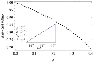
For small but nonzero $q$, it is interesting to compute the correction $\Delta M(q)=M(q)-M(0)$. The equation for the corresponding $\Delta F$ has a form very similar to Eq. (55), with only the “$1$” replaced by an inhomogeneous term, which is proportional to $q^{2}/k^{2}$ for $k\gg q$. The $\Delta M(q)$ resulting from this then vanishes with an exponent that varies with $\beta$. The inset of Fig. 6 illustrates a typical result for $\beta$ not too large; the exponent as a function of $\beta$ is illustrated in the main panel of Fig. 6. One physical consequence of this is that the difference in charge between sublattices for an impurity placed asymmetrically with respect to the sublattices will fall off with a $\beta$-dependent power law at large distances, behavior which may be observable with a local scanning probe.

Figure 6: The exponent in $\Delta M(q)$ as a funciton of $\beta$. Inset: $\Delta M(q)$ for $\beta=0.3$.

The result illustrated in Figs. 5 and 6 have a number of interesting consequences for interacting electrons in undoped graphene. For $\beta<\beta_{c}$, we see that there are indeed power law correlations at long distances in quantities that are in principle measurable, with an exponent varying continuously with $\beta$. This means that the weak-coupling many-body groundstate possesses a basic property of a critical phase. For $\beta>\beta_{c}$ the exponent becomes complex, as in the noninteracting Coulomb implosion problem. In the interacting many-body case, the susceptibility $M(q)$ of Eq. (45) diverges for $k_{0}>0$. This strongly suggests a quantum phase transition to broken symmetry state with staggered charge order Khveshchenko (2001); Gor .

The evolution of this system, from a state with power law correlations to one in which a transition occurs when this power reaches some limiting value, is highly reminiscent of the phenomenology of systems which undergo a KT transition Nelson (2002). In such systems the transition indicates the appearance of a correlation length, which equivalently indicates that a gap develops in the excitation spectrum. This behavior in general should be signaled by a divergence in an appropriate response function. However, the presence of many such divergences as a function of $\beta$ suggests there are different ways to break the symmetry. For a system with finite system size, we expect this chiral symmetry-breaking to occur as $\beta$ increases from small values in a way that is consistent with the first such pole. As we show below, the separation between neighboring poles vanishes only logarithmically as $k_{0}\rightarrow 0$, so that finite size may in fact be important for realistic system sizes.

Nevertheless, the merging of these poles suggests that something else must happen in the thermodynamic limit ref . The merging of these poles as $k_{0}\rightarrow 0$ results in a a continuous function with a branch point at $\beta_{c}$. We interpret this latter non-analytic behavior as the signal of a phase transition. Since it is a result of the merging poles, a natural interpretation is that the instability is into a state involving fluctuations among different realizations of a chiral order parameter which, if quiescent, would produce a gapped exciton phase Khveshchenko (2001); Gor . We speculate that with further increase in $\beta$, one of these orderings could be favored over the others, resulting in a true condensed phase. This would be consistent with results of quantum Monte Carlo calculations dru .

IV.3 An Analytical Model

A fuller understanding of Eq. (55) may be arrived at with a model kernel of the form

$$\tilde{f}_{0}(x)=\theta(1-x)+\frac{1}{x}\theta(x-1).$$ (56)

This has the same behavior as the real kernel at large and small $x$, and is simple enough to allow analytic solutions. We have verified numerically that the results for $F$ and $M$ are qualitatively very similar to those obtained with the correct $f_{0}$.

IV.3.1 Solution by Wiener-Hopf Method

With this model kernel, assuming that the integral converges as $q\to 0$, which will be checked after the solution is found, we obtain, in the $k_{0}\to 0$ limit, the integral equation

$$F\bigg{(}\frac{k}{\Lambda}\bigg{)}-\frac{\beta}{2k}\int\limits_{0}^{\Lambda}dk^{\prime}{\tilde{f}}_{0}\bigg{(}\frac{k^{\prime}}{k}\bigg{)}F\bigg{(}\frac{k^{\prime}}{\Lambda}\bigg{)}=1.$$ (57)

Let us change to more convenient variables via

$$\frac{k}{\Lambda}=e^{-t},\ \ \ \ \frac{k^{\prime}}{\Lambda}=e^{-t^{\prime}}$$ (58)

and rename the function for which we are solving, as well as the kernel,

$$F\bigg{(}\frac{k}{\Lambda}\bigg{)}=g(t),\ \ \ \ {\tilde{f}}_{0}\bigg{(}\frac{k^{\prime}}{k}\bigg{)}=K(t-t^{\prime}),$$ (59)

to obtain the rewritten integral equation

$$g(t)-\frac{\beta}{2}\int\limits_{0}^{\infty}dt^{\prime}e^{t-t^{\prime}}K(t-t^{\prime})g(t^{\prime})=1.$$ (60)

Note that physically meaningful values of $t$ are nonnegative. An important point is that if the limits of integration over $t^{\prime}$ had been $(-\infty,\infty)$ one could have solved the equation trivially by Fourier transformation. Since it is over the half-line one has to use the more sophisticated Wiener-Hopf method M. Hazewinkel (2001).

One first extends the definition of $g$ so that it has the entire real line for its domain, defining

$$g(t)=g_{+}(t)+g_{-}(t),$$ (61)

where $g_{+}(t)$ is nonzero only when $t\geq 0$ and $g_{-}(t)$ is nonzero only for $t\leq 0$. As part of the solution one obtains both $g_{+}$ and $g_{-}$. Defining $R(t)=e^{t}K(t)$ we can now extend the range of integration over $(-\infty,\infty)$ as long as one integrates only $g_{+}$:

$$g_{+}(t)-\frac{\beta}{2}\int\limits_{-\infty}^{\infty}dt^{\prime}R(t-t^{\prime})g_{+}(t^{\prime})=1-g_{-}(t)=r_{+}(t)+r_{-}(t)$$ (62)

where $r_{+}(t)=\Theta(t)$ and $r_{-}(t)=\left[1-g_{-}(t)\right]\Theta(-t)$.

One can now solve the equation by Fourier transformation. The crucial point is that since $g_{+}$ is nonzero only for nonnegative values, if it vanishes as $t\to\infty$, its Fourier transform has poles only in the lower half-plane of complex $\omega$, while $g_{-}$ has poles only in the upper half-plane. This gives us the extra information needed to solve for both $g_{+}$ and $g_{-}$. In general, there is no need for $g_{+}$ to vanish as $t\to\infty$, which would correspond to the original function $F$ vanishing as $k\to 0$. In fact, one expects $F$ to diverge with a power law as $k\to 0$. To incorporate this expectation, we define $g_{+}(t)=e^{st}h_{+}(t)$, with $h_{+}$ vanishing as $t\to\infty$. The new function $h_{+}$ satisfies an integral equation with a modified kernel $R_{s}(t)=e^{-st}R(t)$

$$h_{+}(t)-\frac{\beta}{2}\int\limits_{-\infty}^{\infty}dt^{\prime}R_{s}(t-t^{\prime})h_{+}(t^{\prime})=e^{-st}(r_{+}(t)+r_{-}(t)).$$ (63)

We now take the Fourier transform of both sides, using the explicit form of $\tilde{f}_{0}$, which corresponds to

$$R_{s}(t)=e^{(1-s)t}\Theta(-t)+e^{-st}\Theta(t).$$ (64)

We will abuse notation slightly by using the same name for the function and its Fourier transform, the argument and context serving to distinguish them. Thus, $R_{s}(t)$ has the Fourier transform

$$R_{s}(\omega)=\int\limits_{-\infty}^{\infty}dte^{i\omega t}R_{s}(t)=\frac{1}{i\omega+1-s}+\frac{1}{-i\omega+s}.$$ (65)

The existence of the Fourier transform implies $0\leq s\leq 1$, but does not choose $s$ uniquely. In general, the choice of $s$ determines the class of functions which are allowed as solutions, as we will see explicitly below. Now the equation becomes

$$\bigg{(}\frac{(i\omega)^{2}+i\omega(1-2s)+\beta/2-s(1-s)}{(i\omega-s)(i\omega+1-s)}\bigg{)}h_{+}(\omega)$$

$$=-\frac{1}{i\omega-s}+r_{-}(\omega+is).$$ (66)

To proceed further we separate the prefactor of $h_{+}$ on the left hand side [call it $P(\omega)$] into a product $P(\omega)=P_{+}(\omega)P_{-}(\omega)$, where, by construction, $P_{+}(\omega)$ has zeroes and poles only in the lower half-plane and $P_{-}(\omega)$ has zeroes and poles only in the upper half-plane. We denote the roots of the numerator of $P$ (as a function of $i\omega$) as

$$x_{\pm}=s-\frac{1}{2}\pm\frac{1}{2}\sqrt{1-2\beta}.$$ (67)

One possible choice of $s$ is to make $x_{+}\geq 0,\ \ x_{-}\leq 0$. Let us analyze this case first. This allows us to determine $P_{\pm}$ uniquely.

$$P_{+}(\omega)=\frac{i\omega-x_{+}}{i\omega-s},\ \ \ \ P_{-}(\omega)=\frac{i\omega-x_{-}}{i\omega+1-s}.$$ (68)

Now divide through Eq. (66) by $P_{-}(\omega)$ to obtain

$$P_{+}(\omega)h_{+}(\omega)=-\frac{i\omega+1-s}{(i\omega-x_{-})(i\omega-s)}+\frac{r_{-}(\omega+is)(i\omega+1-s)}{i\omega-x_{-}}.$$ (69)

The first term on the right hand side has poles in both half-planes, and we separate them by partial fractions

$$P_{+}(\omega)h_{+}(\omega)= -\frac{1}{(s-x_{-})(i\omega-s)}$$

$$+\frac{1+x_{-}-s}{(s-x_{-})(i\omega-x_{-})} +\frac{r_{-}(\omega+is)(i\omega+1-s)}{i\omega-x_{-}}.$$ (70)

Since the product $P_{+}h_{+}$ is guaranteed by construction to have poles only in the lower half-plane the terms with the poles in the upper half-plane on the right hand side must separately vanish, and we obtain

$$h_{+}(\omega)=-\frac{1}{(s-x_{-})(i\omega-x_{+})}$$ (71)

Going back to the fictitious “time” variable $t$ and using $g_{+}(t)=e^{st}h_{+}(t)$, we obtain

$$g_{+}(t)=\frac{\Theta(t)e^{(s-x_{+})t}}{(s-x_{-})}$$ (72)

Note that with the definitions of $x_{\pm}$, $s$ drops out of this expression. Translating back to the original variables, we see that $F\propto\big{(}\frac{k}{\Lambda}\big{)}^{-\frac{1}{2}+\frac{1}{2}\sqrt{1-2\beta}}$. It is easily verified that, as assumed in Eq. (57), the integral converges as $k\to 0$. Thus, the Wiener-Hopf method demonstrates the power law behavior of the solution to the integral equation.

Another choice of $s$ would be to make both $x_{\pm}>0$, yielding a solution which diverges more slowly as $k\to 0$. The general solution is a linear combination of both these solutions, and interestingly we see that the equation in its present form does not uniquely specify a particular combination. This ambiguity is lifted by introducing a lower cutoff $k_{0}$ in momentum, corresponding to a finite system size. We show below using an alternate method how this leads to a unique solution.

IV.3.2 Solution of Equivalent Differential Equation

Eq. (55) can also be solved with the model kernel by converting it into a differential equation.

Differentiating Eq. (55) we get

$$F^{\prime}(k)= \frac{\beta}{2}[-\frac{1}{k^{2}}\int_{k_{0}}^{1}dk^{\prime}\tilde{f}_{0}\left(\frac{k^{\prime}}{k}\right)F(k^{\prime})$$

$$+\frac{1}{k}\int_{k}^{1}dk^{\prime}\frac{1}{k^{\prime}}F(k^{\prime})].$$ (73)

Differentiating this equation, we get

$$F^{\prime\prime}(k)= \frac{\beta}{2}[\frac{2}{k^{3}}\int_{k_{0}}^{1}dk^{\prime}\tilde{f}_{0}\left(\frac{k^{\prime}}{k}\right)F(k^{\prime})-\frac{2}{k^{2}}\int_{k}^{1}dk^{\prime}\frac{1}{k^{\prime}}F(k^{\prime})$$

$$-\frac{1}{k^{2}}F(k)],$$ (74)

but from Eq. (73), the first 2 terms in the square brackets are simply $-\frac{2}{k}\frac{2F^{\prime}(k)}{\beta}$. Therefore the differential equation corresponding to Eq. (55) is

$$F^{\prime\prime}(k)+\frac{2}{k}F^{\prime}(k)+\frac{\beta}{2k^{2}}F(k)=0,$$ (75)

which has general solutions of the form

$$F(\tilde{k})=A_{+}\tilde{k}^{\lambda_{+}}+A_{-}\tilde{k}^{\lambda_{-}},$$ (76)

with $\tilde{k}=k/\Lambda$, $\lambda_{\pm}=\frac{-1\pm\gamma}{2}$, and $\gamma=\sqrt{1-2\beta}$. The coefficients $A_{\pm}$ are determined by substituting Eq. 76 back into the integral equation. This results in power law behavior for $k\gg k_{0}$, with exponent $\lambda_{+}$, which goes from real to complex when $\beta$ exceeds 1/2. Moreover, $M(q\rightarrow 0)$ may be evaluated, yielding

$$M(0)=\frac{\Lambda}{v_{F}}\frac{2-2\tilde{k}_{0}^{\gamma}}{1+\gamma-\beta+\tilde{k}_{0}^{\gamma}(-1+\gamma+\beta)}.$$ (77)

This has poles for $\beta>1/2$ when

$$\sqrt{2\beta-1}\ln{\tilde{k}_{0}}=2\arctan{\frac{\sqrt{2\beta-1}}{1-\beta}}+2\pi n,$$ (78)

with integer $n$ and $0<\arctan{(x)}<\pi$. Note that the distance between poles vanishes logarithmically as $\tilde{k}_{0}\rightarrow 0$, as discussed above. Furthermore, for $\beta>1/2$, $\tilde{k}_{0}^{\gamma}$ becomes ill-defined unless an infinitesimal imaginary part is introduced in $\beta$, so that $\beta=1/2$ becomes a branch point for $M(0)$. We interpret this as the signal of a phase transition in the thermodynamic limit, since $M(0)$ need not be real and positive beyond this point.

V density response

In this final section we return to another measurable quantity, the density response function. To be concrete we will use our result to compute the induced charge around a Coulomb impurity, which generates the potential $Ze/\epsilon r$, where $e\equiv|e|$. Our procedure is to first solve Eq. (IV.1) numerically, from which we compute the (static) irreducible polarizability

$$\Pi(\vec{q})=i\int\frac{d^{2}k}{(2\pi)^{2}}\tilde{K}_{\beta_{2}\beta_{1}\alpha\alpha}\tilde{\Gamma}_{\beta_{1}\beta_{2}}(\vec{k},\vec{q}).$$ (79)

The density response function is then computed by an RPA sum fet , except that instead of using the non-interacting polarizability we use our irreducible polarizability, which includes excitonic corrections via the ladder diagrams. The result of this takes the form

$$D(q)=\frac{-\Pi(q)}{1+\Pi(q)U_{C}(q)},$$ (80)

where $U_{C}(q)=2\pi\beta v_{F}/q$ is the Coulomb interaction. Finally, the Fourier transform of the induced electron density is given by

$$\delta n(q)=D(q)\phi_{\text{ext}}(q).$$ (81)

In the Coulomb impurity case, the external potential $\phi_{\text{ext}}(q)=-ZU_{C}(q)$.

To find numerical solutions to Eq. (IV.1), we discretize the allowed values of momentum $\vec{k}$ and $\vec{q}$, and replace integrations by sums over the grid of allowed momenta. In doing this, some subtleties arise. Since we cannot retain an infinite number of momentum points, we must confine the sums to a finite region, most conveniently taken to be square. If we use the MDF spectrum and wavefunctions (needed to construct $\tilde{K}$) in Eq. IV.1 in this “Brillouin zone”, the former will be periodic but not the latter. The discontinuity in wavefunctions leads to spurious oscillations in the final result. In principle this can be overcome by simulating the system on a honeycomb lattice and using the full tight-binding spectrum and wavefunctions for graphene. However, this is numerically costly and unnecessary, because the low energy physics is almost entirely determined by the wavefunctions and spectra near the Dirac cones. Moveover, since Coulomb interactions are relatively weak at short wavelengths, one can neglect the intervalley scattering, so that it should be sufficient to consider only one Dirac cone, whereas a simulation of a honeycomb lattice would force us to include two due to fermion doubling Neto et al. (2009).

As a compromise we consider models that have simpler bandstructures than graphene but still have a Dirac cone. One such model arises in the theory of the surface of a topological insulator Qi et al. (2006, 2008), and has the form ($\hbar v_{F}=1$)

$$H= \sum_{n}\left[\vec{c}_{n}^{\dagger}\frac{\sigma_{z}-i\sigma_{x}}{2}\vec{c}_{n+\hat{x}}+\vec{c}_{n}^{\dagger}\frac{\sigma_{z}-i\sigma_{y}}{2}\vec{c}_{n+\hat{y}}+h.c.\right]$$ (82)

$$+m\sum_{n}\vec{c}_{n}^{\dagger}\sigma_{z}\vec{c}_{n}$$

$$= \sum_{\vec{k}}\vec{c}^{\dagger}_{\vec{k}}h(\vec{k})\vec{c}_{\vec{k}},$$ (83)

where

$$h(\vec{k})=(\sin k_{x})\sigma_{x}+(\sin k_{y})\sigma_{y}+\left(m+\cos k_{x}+\cos k_{y}\right)\sigma_{z}.$$ (84)

This is a model defined on a square lattice, with each site supporting a two-component vector of localized orbitals combined into annihilation operators $\vec{c}_{n}$, and with the sum over $n$ running through all the lattice sites. The crystal momentum $\vec{k}$ is measured in units of $1/a$, with $a$ the lattice constant. For $m=2$, there is a single Dirac point at the center of the BZ, and the spinor structure in the vicinity of this point is the same as near the Dirac points in graphene. Thus we expect this model to reproduce the low-energy behavior of graphene. We adopt this model for our numerical solution of Eq. (IV.1).

A second subtlety arises in the doped case. For example, when the chemical potential $\mu>0$, the quantity $\tilde{K}$ in Eq. (IV.1) takes the form

$$\tilde{K}^{\mu>0}_{\alpha_{1}\beta_{1},\alpha_{2}\beta_{2}}(\vec{k},\vec{q})=$$ (85)

$$\frac{\left[\theta(\varepsilon_{\vec{k}}-\mu)-\theta(\varepsilon_{\vec{k}+\vec{q}}-\mu)\right]g^{+}_{\beta_{1}\beta_{2}}(\vec{k})g^{+}_{\alpha_{2}\alpha_{1}}(\vec{k}+\vec{q})}{\varepsilon_{\vec{k}}-\varepsilon_{\vec{k}+\vec{q}}}$$

$$+\frac{\theta(\varepsilon_{\vec{k}}-\mu)g^{+}_{\beta_{1}\beta_{2}}(\vec{k})g^{-}_{\alpha_{2}\alpha_{1}}(\vec{k}+\vec{q})}{\varepsilon_{\vec{k}}+\varepsilon_{\vec{k}+\vec{q}}}$$

$$+\frac{\theta(\varepsilon_{\vec{k}+\vec{q}}-\mu)g^{-}_{\beta_{1}\beta_{2}}(\vec{k})g^{+}_{\alpha_{2}\alpha_{1}}(\vec{k}+\vec{q})}{\varepsilon_{\vec{k}}+\varepsilon_{\vec{k}+\vec{q}}},$$

where $\varepsilon_{\vec{k}}$ is the positive eigenvalue of $h(\vec{k})$ and $g^{\pm}_{\alpha\beta}(\vec{k})=(\eta^{\pm}_{\vec{k}})_{\alpha}(\eta^{\pm}_{\vec{k}})_{\beta}^{*}$, with $\eta^{\pm}_{\vec{k}}$ being the eigenvectors of $h(\vec{k})$ corresponding to $\pm\varepsilon_{\vec{k}}$ respectively.

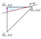
Because of the step functions, a naive numerical integration by a discrete summation works poorly, because the function being integrated is not smooth on the scale of the grid. This problem may be overcome using the Triangular Linear Analytic (TLA) methodfir ; sec . We divide the square Brillouin zone into small squares, and each small square is further subdivided into two right trangles along one of the diagonals. Weights for the integrand can then be assigned at the corners of the triangles employing the parameterization formulas in Ref. sec, tri . Using this weighting scheme to approximate the integrals gives far better results than a naive lattice sum.

Finally, we note that $U(q)$ in Eq. (IV.1) is better represented by the RPA screened Coulomb interaction than the bare Coulomb interaction, i.e.,

$$U(q)=\frac{U_{C}(q)}{1+\Pi^{\text{RPA}}(q)U_{C}(q)}.$$ (86)

The irreducible RPA polarizability $\Pi^{\text{RPA}}(q)$ has been calculated by a number of authors (see, e.g. Refs. Hwang and Das Sarma, 2007 and Wunsch et al., 2006). For the case of undoped graphene there is no qualitative difference between using screened or unscreened Coulomb interactions in the ladder rungs, because the functional forms of $U(q)$ and $U_{C}(q)$ are the same, and only the effective value of $\beta$ is renormalized. When $\mu\neq 0$, however, the Fermi surface introduces a length scale into the problem, allowing genuine screening of the Coulomb interaction at long distances. This can be modeled by using a contact interaction on the ladder rungs Brey and Halperin (1989); Wunsch et al. (2006) although we find this introduces problems at large wavevectors, as we describe below.

Figure 7: (Color online) Total induced electron number density divided by $Z$ in the undoped case.

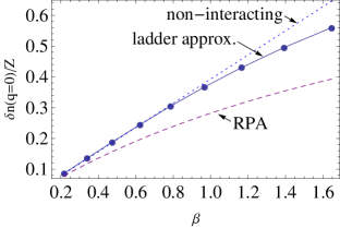
Fig. 7 shows the total induced electron number density in the undoped case, together with the RPA result

$$\frac{\delta n^{\text{RPA}}(q=0)}{Z}=\frac{\Pi^{\text{RPA}}(q)U_{C}(q)}{1+\Pi^{\text{RPA}}(q)U_{C}(q)}=\frac{\frac{\pi\beta}{8}}{1+\frac{\pi\beta}{8}}$$ (87)

and the non-interacting result

$$\frac{\delta n^{\text{non}}(q=0)}{Z}=\Pi^{\text{RPA}}(q)U_{C}(q)=\frac{\pi\beta}{8}$$ (88)

for comparison. It is clear that the non-interacting result exceeds 1 for $\beta>8/\pi$, while the RPA result approaches 1 as $\beta\rightarrow\infty$. Results for the total induced charge using the RPA and the ladder approximation are not qualitatively different. The ladder approximation result is larger than the RPA result, and the difference increases with $\beta$.

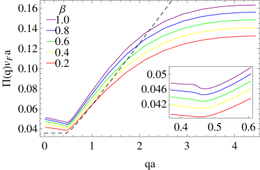
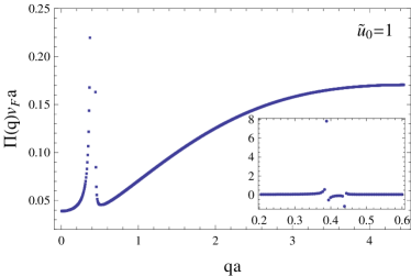
For doped graphene, any charged impurity will induce an equal and opposite screening charge, both in the RPA and when exciton corrections are included. However, we find in the latter case a strong quantitative difference between the two in the shape of the screening cloud. This is due to the effect of the exciton corrections on the irreducible polarizability in the doped case, illustrated in Fig. 8. For small $\beta$, $\Pi$ is close to the RPA result for MDF as expected, except that the for $q<2k_{F}$ there is a negative slope, and for $q$ close to the Brillouin zone boundary it is significantly below the RPA result for MDF, simply because of the presence of the zone boundary. For larger $\beta$, the curve is higher and the deviation from the RPA result for MDF is larger, and for the largest $\beta$, an additional “hump” structure develops just below $2k_{F}$, as illustrated in the inset of Fig. 8. We will consider this extra structure in more detail below.

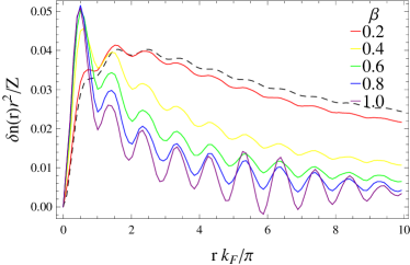
The cusp in the density response function at $q=2k_{F}$ is well-known to induce Friedel oscillations fri . The change in shape of the irreducible polarizability near $2k_{F}$ essentially deepens this cusp, leading to an enhancement of these oscillations. Fig. 9 shows the induced charge distribution, illustrating this enhancement. We also note that with the exciton corrections included, the induced charge density falls off somewhat faster than the RPA result.

Figure 8: (Color online) The continuous color curves are the irreducible polarizability $\Pi(q)$ for the model Hamiltonian Eq. (82) in the doped case, with RPA screened Coulomb interaction as the rungs of the ladders, for $\beta=0.2,0.4,\dots,1.0$, with higher curves corresponding to higher $\beta$. The dashed black curve is the RPA result for MDF for comparison. The inset is a blow-up showing the developing structure just below $q=2k_{F}$. For all the numerical results shown in this figure $\mu=0.225\hbar v_{F}/a$.

Figure 9: (Color online) Induced electron number density (times $r^{2}/Z$) as a function of distance $r$ from the impurity in the doped case. On the far right side, from top to bottom, the curves correspond to $\beta=0.2,0.4,\dots,1.0$. For comparison, the dashed line is the RPA result with $\beta=0.2$.

We can also carry out the calculation with contact interactions as rungs of the ladders, i.e. $U(q)=u_{0}$ in Eq. (IV.1), which then becomes

$$\tilde{\Gamma}_{\alpha_{2}\beta_{2}}({\vec{q}})=\delta_{\alpha_{2}\beta_{2}}+$$

$$u_{0}\left[\int\frac{d^{2}q^{\prime}}{(2\pi)^{2}}\tilde{K}_{\alpha_{2}\beta_{2}\gamma_{1}\gamma_{2}}(\vec{q}^{\prime},\vec{q})\right]\tilde{\Gamma}_{\gamma_{1}\gamma_{2}}(\vec{q}).$$

This is a considerable simplification relative to the equation we had to solve for the RPA-screened Coulomb interaction; we now have a simple set of linear equations for $\tilde{\Gamma}_{\alpha_{2}\beta_{2}}({\vec{q}})$. The resulting irreducible polarizability is

$$\Pi(q)=\frac{\frac{1}{2\pi}\Pi^{\text{RPA}}(q)}{1-\frac{u_{0}}{4\pi}\Pi^{\text{RPA}}(q)}.$$ (90)

This is plotted in Fig. 10 for the doped case. We see that the simpler contact interaction does not enhance the cusp at $q=2k_{F}$, suggesting that the correct long-distance form of the screened Coulomb potential is an important ingredient in obtaining this behavior. Note also that because of the minus sign in the denominator of Eq. (90) and the monotonic increase of $\Pi^{\text{RPA}}(q)$ at large $q$, there is a pole at some sufficiently large $q$ for any positive $u_{0}$, suggesting an instability in this model which is absent for the more realistic $U(q)$.

Figure 10: (Color online) Irreducible polarizability in the ladder approximation with contact interaction as the rungs of the ladders, for MDF in the doped case [Eq. (90)]. $\tilde{u}_{0}\equiv u_{0}k_{F}/v_{F}$. The inset is the same plot with a larger range of $q$.

Figure 11: (Color online) Numerical result for the irreducible polarizability in the ladder approximation with contact interaction as the rungs of the ladders, for the model Eq. (82) in the doped case. The insets are the blow-up around $q=2k_{F}$. (a)$\tilde{u}_{0}=0.2,0.4,0.6,0.8,0.9$; (b)$\tilde{u}_{0}=1.0$.

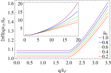
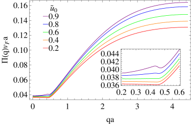
We can also obtain results for rungs with contact interactions numerically for our topological insulator surface model, Eq. (82), illustrated in Fig. 11. Comparison between this and the nearly analytic results for MDF’s allow us to assess which features may be introduced by going from the latter to the former. As we can see, the curves are very similar in overall scale to those when the interaction is the RPA screened Coulomb interaction (Fig. 8). Note however that the deepening of the $2k_{F}$ cusp is absent in both the numerical result and the analytical one, suggesting that our numerical results are reasonably accurate at small $q$. However, we note that for the largest values of $\beta$, extra structure near $2k_{F}$ develops that appears analogous to what we found in the Coulomb case. This structure appears only in the result for the model Eq. (82), not in the analytical result for MDF’s. It is thus reasonable to assume that the analogous structure in the RPA screened Coulomb interaction case is peculiar to Eq. (82) as well. It is interesting to speculate then that one may be able to distinguish the Dirac cone in the graphene system from that of at the surface of a topological insulator through such structure at very large $\beta$.

Finally, in Fig. 11 we illustrate that divergent behavior emerges when $u_{0}$ is sufficiently large, which evolves into a double pole from the “hump” structure below $2k_{F}$. This suggests the system becomes unstable for contact interactions of sufficiently large magnitude, a behavior that occurs as we observed above for any $u_{0}$ when MDF’s are subject to contact interactions. (Note, however, in this case the instability sets in for $q<2k_{F}$, whereas for contact interactions the instability occurs at much larger $q$ when the interaction is weak.) While this behavior is absent in the screened Coulomb interaction case, it is possible that at very small distances where the atomic orbital physics becomes relevant such a contact model becomes appropriate. Since this instability appears in the density-density response function this naively suggests that there is a phase transition into a charge-density wave. However, other transitions – spin or valley density waves, for example – may preempt this transition. We leave the nature of such an instability and its applicability to real graphene as open questions her .

VI conclusion

In this work we have investigated excitonic effects for graphene with Coulomb interactions, as modeled by massless Dirac fermions. We have shown that there is power law behavior in a general 4-leg vertex function in the particle-hole channel. The exponent becomes complex as the coupling constant $\beta$ is increased above a critical value. This is analogous to what happens in the problem of a single MDF interacting with a charged impurity. This non-analytic behavior can be canceled away for certain combinations of the vertex function, and we find in particular that it is absent in the density-density response function. It is however retained in a sublattice antisymmetric response function. Although the power law behavior originates due to short length scale physics (close approaches of particle-hole pairs), it impacts the physics at large distances because of the absence of a length scale in the Hamiltonian. For finite size systems the transition appears to be one with broken chiral symmetry, inducing a gap in the spectrum; however, this interpretation breaks down in the thermodynamic limit. We speculate that in this case the transition involves the formation of a mass gap which fluctuates among different possible forms, and is a precursor to a true broken symmetry state which emerges at still larger values of the coupling $\beta$.

We have also calculated the density response in the ladder approximation numerically using a simplified model Hamiltonian that occurs in the context of topological insulators, which has only one Dirac point and a square Brillouin zone. The calculation was carried out for both undoped and doped cases. In the latter case we compared results for RPA screened Coulomb interactions and contact interactions in the rungs of the ladders. While we expect the former interaction to be more realistic, both interactions in many respects give similar results. For Coulomb interactions, we find a strongly enhanced cusp in the irreducible polarizability at $2k_{F}$, which leads to much stronger Friedel oscillations than expected from the RPA. We also find a hump-like structure at stronger interaction scales just below $2k_{F}$. For contact interactions this hump evolves into poles with increasing interaction strength, whereas no pole is seen for RPA screened Coulomb interactions in the range of $\beta$ we have studied. We presented evidence that the extra structure is peculiar to our model Hamiltonian, suggesting it may be present at the surface of a topological insulator. Finally, we note that with contact interactions, MDF’s do contain a pole at larger $q$ for any positive $u_{0}$, suggesting a short wavelength instability.

Appendix A

In this Appendix, we discuss some details of the TLA method. This may be viewed as a two-dimensional version of the “tetrahedron method” Jepsen and Andersen (1971); Lehmann and Taut (1972) which is widely applied for Brillouin zone integrations of three dimensional systems. As mentioned in Ref. sec, , when using linear interpolation, the surfaces $e=\varepsilon(x,y)$ (in this Appendix $x\equiv k_{x}$ and $y\equiv k_{y}$) are straight lines and the parameterizations are easily given (with $e$ being one of the parameters). There are two cases: $e<\varepsilon_{2}$ (but larger than $\varepsilon_{1}$) and $e>\varepsilon_{2}$ (but smaller than $\varepsilon_{3}$). The parameterizations are given by Eqs. (14) and (16) in Ref. sec, , respectively. For convenience we reproduce them here.

$$\vec{k}= \vec{k}_{3}+\frac{e-\varepsilon_{3}}{\varepsilon_{3}-\varepsilon_{1}}(\vec{k}_{3}-\vec{k}_{1})$$

$$+u\left[\frac{e-\varepsilon_{3}}{\varepsilon_{3}-\varepsilon_{2}}(\vec{k}_{3}-\vec{k}_{2})-\frac{e-\varepsilon_{3}}{\varepsilon_{3}-\varepsilon_{1}}(\vec{k}_{3}-\vec{k}_{1})\right]$$ (91)

for $e>\varepsilon_{2}$, and

$$\vec{k}= \vec{k}_{1}+\frac{e-\varepsilon_{1}}{\varepsilon_{3}-\varepsilon_{1}}(\vec{k}_{3}-\vec{k}_{1})$$

$$+u\left[\frac{e-\varepsilon_{1}}{\varepsilon_{2}-\varepsilon_{1}}(\vec{k}_{2}-\vec{k}_{1})-\frac{e-\varepsilon_{1}}{\varepsilon_{3}-\varepsilon_{1}}(\vec{k}_{3}-\vec{k}_{1})\right]$$ (92)

for $e<\varepsilon_{2}$; in both cases $0\leqslant u\leqslant 1$.

Figure 12: (Color online) Illustrations for (a) case (ii) and (b) case (iii). In both subfigures the red and purple arrows label the directions of increasing $e$ and $u$ respectively. However, while they correspond to Eq. (91) in (a), in (b) they correspond to Eq. (92).

Our goal is to express the integral over a basic triangle in terms of the values of $\varepsilon(x,y)$ and the integrand at the three corners of the triangle, i.e.

$$I(\mu)=\int_{\bigtriangleup}d^{2}k\theta(\varepsilon_{\vec{k}}-\mu)f(\vec{k})\approx\sum_{i=1}^{3}w_{i}(\varepsilon_{1},\varepsilon_{2},\varepsilon_{3},\mu)f(\vec{k}_{i}),$$ (93)

where $\int_{\triangle}$ means integration over the triangle, $w_{i},\,i=1,2,3$ are the weights at the three corners (remember that the corners are labeled so that $\varepsilon_{1}<\varepsilon_{2}<\varepsilon_{3}$). We will also use the shorthand $f_{i}\equiv f(\vec{k}_{i})$ below.

There are four possibilities regarding the value of $\mu$ as compared to $\varepsilon_{1},\varepsilon_{2},\varepsilon_{3}$:

(i) $\mu\geqslant\varepsilon_{3}$:

This is trivial and the result is $w_{i}=0,\,i=1,2,3$.

(ii) $\varepsilon_{2}\leqslant\mu<\varepsilon_{3}$:

In this case, we need to use Eq. (91) for the parameterization, and

$$I(\mu)\approx\int^{\prime}d^{2}kf(\vec{k}(e,u))=\int_{\mu}^{\varepsilon_{3}}de\int_{0}^{1}du\frac{2A(\varepsilon_{3}-e)}{(\varepsilon_{3}-\varepsilon_{2})(\varepsilon_{3}-\varepsilon_{1})}f(\vec{k}(e,u))\equiv I_{\text{I}}(\mu),$$ (94)

where $\int^{\prime}$ means integration over the uppermost (light blue) triangle in Fig. 12, and the extra factor in the integrand is just the Jacobian, with $A$ being the area of the triangle 123 (not the shaded triangle).

We intepolate $f$ linearly, i.e.

$$f(x,y)\approx p_{1}+p_{2}x+p_{3}y\equiv\sum_{i=1}^{3}p_{i}g_{i}(x,y),$$ (95)

where $g_{1}\equiv 1$, $g_{2}\equiv x$, $g_{3}\equiv y$, and the coefficients $p_{i},\,i=1,2,3$ are determined by solving the equations $\sum_{i=1}^{3}p_{i}g_{i}(x_{j},y_{j})=f_{j}$. The result is

$$p_{1}=\frac{(x_{3}y_{2}-x_{2}y_{3})f_{1}+(x_{1}y_{3}-x_{3}y_{1})f_{2}+(x_{2}y_{1}-x_{1}y_{2})f_{3}}{x_{2}y_{1}-x_{3}y_{1}-x_{1}y_{2}+x_{3}y_{2}+x_{1}y_{3}-x_{2}y_{3}},$$ (96)

$p_{2}$ and $p_{3}$ have the same denominator but with the numerator being $[(y_{3}-y_{2})f_{1}+(y_{1}-y_{3})f_{2}+(y_{2}-y_{1})f_{3}]$ for $p_{2}$ and $[(x_{2}-x_{3})f_{1}+(x_{3}-x_{1})f_{2}+(x_{1}-x_{2})f_{3}]$ for $p_{3}$.

$$I_{\text{I}}(\mu)\approx\sum_{i=1}^{3}Ap_{i}\int_{\mu}^{\varepsilon_{3}}de\int_{0}^{1}du\frac{2(\varepsilon_{3}-e)}{(\varepsilon_{3}-\varepsilon_{2})(\varepsilon_{3}-\varepsilon_{1})}g_{i}\equiv\sum_{i=1}^{3}Ap_{i}I_{\text{I}}(\mu)_{i}.$$ (97)

The results of the integrations are

$$I_{\text{I}}(\mu)_{1} =\int_{\mu}^{\varepsilon_{3}}de\frac{2(\varepsilon_{3}-e)}{(\varepsilon_{3}-\varepsilon_{2})(\varepsilon_{3}-\varepsilon_{1})}\int_{0}^{1}du=\frac{(\varepsilon_{3}-\mu)^{2}}{(\varepsilon_{3}-\varepsilon_{2})(\varepsilon_{3}-\varepsilon_{1})},$$ (98)

$$I_{\text{I}}(\mu)_{2} =\int_{\mu}^{\varepsilon_{3}}de\frac{2(\varepsilon_{3}-e)}{(\varepsilon_{3}-\varepsilon_{2})(\varepsilon_{3}-\varepsilon_{1})}\int_{0}^{1}du\left\{x_{3}+\frac{e-\varepsilon_{3}}{\varepsilon_{3}-\varepsilon_{1}}(x_{3}-x_{1})+u\left[\frac{e-\varepsilon_{3}}{\varepsilon_{3}-\varepsilon_{2}}(x_{3}-x_{2})-\frac{e-\varepsilon_{3}}{\varepsilon_{3}-\varepsilon_{1}}(x_{3}-x_{1})\right]\right\}$$

$$=\frac{(\varepsilon_{3}-\mu)^{2}}{(\varepsilon_{3}-\varepsilon_{2})(\varepsilon_{3}-\varepsilon_{1})}\left[x_{3}-\frac{1}{3}(\varepsilon_{3}-\mu)\left(\frac{x_{3}-x_{1}}{\varepsilon_{3}-\varepsilon_{1}}+\frac{x_{3}-x_{2}}{\varepsilon_{3}-\varepsilon_{2}}\right)\right],$$ (99)

and $I_{\text{I}}(\mu)_{3}$ is the same as $I_{\text{I}}(\mu)_{2}$ but with the $x$’s replaced by $y$’s. Finally, we have

$$w_{1}=\frac{A\left[(x_{3}y_{2}-x_{2}y_{3})I_{\text{I}}(\mu)_{1}+(y_{3}-y_{2})I_{\text{I}}(\mu)_{2}+(x_{2}-x_{3})I_{\text{I}}(\mu)_{3}\right]}{x_{2}y_{1}-x_{3}y_{1}-x_{1}y_{2}+x_{3}y_{2}+x_{1}y_{3}-x_{2}y_{3}},$$ (100)

$w_{2}$ and $w_{3}$ have the same denominator but with the numerator being $A[(x_{1}y_{3}-x_{3}y_{1})I_{\text{I}}(\mu)_{1}+(y_{1}-y_{3})I_{\text{I}}(\mu)_{2}+(x_{3}-x_{1})I_{\text{I}}(\mu)_{3}]$ for $w_{2}$ and $A[(x_{2}y_{1}-x_{1}y_{2})I_{\text{I}}(\mu)_{1}+(y_{2}-y_{1})I_{\text{I}}(\mu)_{2}+(x_{1}-x_{2})I_{\text{I}}(\mu)_{3}]$ for $w_{3}$.

(iii)$\varepsilon_{1}<\mu<\varepsilon_{2}$

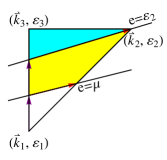
In this case, $I(\mu)\approx\int^{\prime\prime}d^{2}kf(\vec{k}(e,u))$ where the integration is over the uppermost (cyan) triangle and the yellow quadrilateral in Fig. 12. The former is approximately the same (to linear order of the size of the basic triangles) as $I_{\text{I}}(\varepsilon_{2})$, while the latter is

$$I_{\text{II}}(\mu)\approx\sum_{i=1}^{3}Ap_{i}\int_{\mu}^{\varepsilon_{2}}de\frac{2(e-\varepsilon_{1})}{(\varepsilon_{2}-\varepsilon_{1})(\varepsilon_{3}-\varepsilon_{1})}\int_{0}^{1}dug_{i}\equiv\sum_{i=1}^{3}Ap_{i}I_{\text{II}}(\mu)_{i}.$$ (101)

The $I_{\text{I}}(\mu)_{i}$’s in the formula given above for case (ii) should be replaced by

$$I_{\text{I}}(\varepsilon_{2})_{1}+I_{\text{II}}(\mu)_{1} = \frac{\varepsilon_{3}-\varepsilon_{2}}{\varepsilon_{3}-\varepsilon_{1}}+\int_{\mu}^{\varepsilon_{2}}de\frac{2(e-\varepsilon_{1})}{(\varepsilon_{2}-\varepsilon_{1})(\varepsilon_{3}-\varepsilon_{1})}\int_{0}^{1}du$$ (102)

$$= \frac{\varepsilon_{3}-\varepsilon_{2}}{\varepsilon_{3}-\varepsilon_{1}}+\frac{(\varepsilon_{2}-\varepsilon_{1})^{2}-(\mu-\varepsilon_{1})^{2}}{(\varepsilon_{2}-\varepsilon_{1})(\varepsilon_{3}-\varepsilon_{1})},$$

$$I_{\text{I}}(\varepsilon_{2})_{2}+I_{\text{II}}(\mu)_{2} = \frac{\varepsilon_{3}-\varepsilon_{2}}{\varepsilon_{3}-\varepsilon_{1}}\left[x_{3}-\frac{1}{3}(\varepsilon_{3}-\varepsilon_{2})\left(\frac{x_{3}-x_{1}}{\varepsilon_{3}-\varepsilon_{1}}+\frac{x_{3}-x_{2}}{\varepsilon_{3}-\varepsilon_{2}}\right)\right]+\int_{\mu}^{\varepsilon_{2}}de\frac{2(e-\varepsilon_{1})}{(\varepsilon_{2}-\varepsilon_{1})(\varepsilon_{3}-\varepsilon_{1})}$$ (103)

$$\times\int_{0}^{1}du\left\{x_{1}+\frac{e-\varepsilon_{1}}{\varepsilon_{3}-\varepsilon_{1}}(x_{3}-x_{1})+u\left[\frac{e-\varepsilon_{1}}{\varepsilon_{2}-\varepsilon_{1}}(x_{2}-x_{1})-\frac{e-\varepsilon_{1}}{\varepsilon_{3}-\varepsilon_{1}}(x_{3}-x_{1})\right]\right\}$$

$$= \frac{\varepsilon_{3}-\varepsilon_{2}}{\varepsilon_{3}-\varepsilon_{1}}\left[x_{3}-\frac{1}{3}(\varepsilon_{3}-\varepsilon_{2})\left(\frac{x_{3}-x_{1}}{\varepsilon_{3}-\varepsilon_{1}}+\frac{x_{3}-x_{2}}{\varepsilon_{3}-\varepsilon_{2}}\right)\right]+\frac{1}{(\varepsilon_{2}-\varepsilon_{1})(\varepsilon_{3}-\varepsilon_{1})}$$

$$\times\left\{\left[(\varepsilon_{2}-\varepsilon_{1})^{2}-(\mu-\varepsilon_{1})^{2}\right]x_{1}+\frac{1}{3}\left[(\varepsilon_{2}-\varepsilon_{1})^{3}-(\mu-\varepsilon_{1})^{3}\right]\left(\frac{x_{2}-x_{1}}{\varepsilon_{2}-\varepsilon_{1}}+\frac{x_{3}-x_{1}}{\varepsilon_{3}-\varepsilon_{1}}\right)\right\}$$

and $I_{\text{II}}(\varepsilon_{2})_{3}+I_{\text{II}}(\mu)_{3}$, which is the same as $I_{\text{I}}(\varepsilon_{2})_{2}+I_{\text{II}}(\mu)_{2}$ but with the $x$’s replaced by $y$’s.

(iv)$\mu\leqslant\varepsilon_{1}$

This case is trivial too, we simply have $w_{1}=w_{2}=w_{3}=1/3$.

References

- Neto et al. (2009) A. C. Neto, F.Guinea, N.M.R.Peres, K.S.Novoselov, and A.K.Geim, Rev. Mod. Phys. 81, 109 (2009).
- (2) S. Das Sarma, S. Adam, E.H. Hwang and E. Rossi, arXiv:1003.4731.
- Gonzalez et al. (1994) J. Gonzalez, F.Guinea, and M. Vozmediano, Nuc. Phys. B 424, 595 (1994).
- (4) J. E. Drut and T. A. Lähde, Phys. Rev. Lett. 102, 026802 (2009); Phys. Rev. B 79, 165425 (2009); ibid. 79, 241405 (2009).
- (5) A. V. Shytov and M. I. Katsnelson and L. S. Levitov, Phys. Rev. Lett. 99, 236801 (2007).
- per (a) V. M. Pereira and J. Nilsson and A. H. Castro Neto, Phys. Rev. Lett. 99, 166802 (2007).
- (7) R. R. Biswas and S. Sachdev and D. T. Son, Phys. Rev. B 76, 205122 (2007).
- (8) I. S. Terekhov and A. I. Milstein and V. N. Kotov and O. P. Sushkov, Phys. Rev. Lett. 100, 076803 (2008).
- per (b) V. M. Pereira and V. N. Kotov and A. H. Castro Neto, Phys. Rev. B 78, 085101 (2008).
- (10) V. N. Kotov and V. M. Pereira and B. Uchoa, Phys. Rev. B 78, 075433 (2008).
- Schwabl (2008) F. Schwabl, in Advanced Quantum Mechanics (Springer-Verlag, Heidelberg, 2008).
- (12) A. L. Fetter and J. D. Walecka, Quantum Theory of Many-Particle Systems, Chap. 4, §11 (Dover, 2003).
- Nelson (2002) D. Nelson, in Defects and Geometry in Condensed Matter Physics (Cambridge University Press, New York, 2002).
- Wang et al. (2010) J. Wang, H. A. Fertig, and G. Murthy, Phys. Rev. Lett. 104, 186401 (2010).
- Cheianov and Falko (2006) V. Cheianov and V. Falko, Phys. Rev. Lett. 97, 226801 (2006).
- Brey et al. (2007) L. Brey, H. Fertig, and S. Das Sarma, Phys. Rev. Lett. 99, 116802 (2007).
- Wehling et al. (2007) T. Wehling, A. V. Balatsky, M. I. Katsnelson, A. I. Lichtenstein, K. Scharnberg, and R. Wiesendanger, Phys. Rev. B 75, 125425 (2007).
- Yazyev and Helm (2007) O. Yazyev and L. Helm, Phys. Rev. B 75, 125408 (2007).
- Khveshchenko (2001) D. V. Khveshchenko, Phys. Rev. Lett. 87, 246802 (2001).
- (20) E. V. Gorbar, V. P. Gusynin, V. A. Miransky, and I. A. Shovkovy, Phys. Rev. B 66, 045108 (2002).
- Merzbacher (1970) E. Merzbacher, Quantum Mechanics, 2nd Edition (Wiley, New York, 1970).
- (22) W. H. Press et al., Numerical Recipes, 3rd Edition (Cambridge University Press, 2007).
- (23) The authors thank the anonymous referee of Ref. Wang et al., 2010 for pointing this out.
- M. Hazewinkel (2001) E. M. Hazewinkel, The Wiener-Hopf Method (Springer, 2001).
- Qi et al. (2006) X.-L. Qi, Y.-S. Wu, and S.-C. Zhang, Phys. Rev. B 74, 045125 (2006).
- Qi et al. (2008) X.-L. Qi, T. L. Hughes, and S.-C. Zhang, Phys. Rev. B 78, 195424 (2008).
- (27) J. A. Ashraff and P. D. Loly, J. Phys. C 20, 4823 (1987).
- (28) G. Wiesenekker, G. te Velde and E. J. Baerends, J. Phys. C 21, 4263 (1988).
- (29) The formulas provided in Ref. sec, require some modification for this application. When a triangle is completely “occupied” (i.e., all three points inside the Fermi surface), the weights are still dependent on or [for and terms respectively], where labels the corners. If there are grid points where and the weights calculated using and are different (which in general is the case), then the first line in Eq. (85) is infinite. To avoid this situation, we set the weights at the 3 corners to 1/3 of the area of a triangle if the triangle is fully occupied, i.e. , . After calculating the weights at every grid point, we divide each small square into triangles along the other diagonal and re-calculate the weights. The final weights are the averages of the results of the two calculations. See the appendix for more detail.
- Hwang and Das Sarma (2007) E. H. Hwang and S. Das Sarma, Phys. Rev. B 75, 205418 (2007).
- Wunsch et al. (2006) B. Wunsch, T. Stauber, F. Sols, and F. Guinea, New J. Phys. 8, 318 (2006).
- Brey and Halperin (1989) L. Brey and B. Halperin, Phys. Rev. B. 40, 11634 (1989).
- (33) See, for example, Ref. Brey et al., 2007 and references therein.
- (34) See, for example, I.F. Herbut, V. Juricic, and B. Roy, Phys. Rev. B 79, 085116 (2009) and references therein.
- Jepsen and Andersen (1971) O. Jepsen and O. Andersen, Solid State Commun. 9, 1763 (1971).
- Lehmann and Taut (1972) G. Lehmann and M. Taut, Phys. Status Solidi B 54 (1972).