Robust $H_{\infty}$ Filter Design for Lipschitz Nonlinear Systems via Multiobjective Optimization

Abstract

In this paper, a new method of $H_{\infty}$ observer design for Lipschitz nonlinear systems is proposed in the form of an LMI optimization problem. The proposed observer has guaranteed decay rate (exponential convergence) and is robust against unknown exogenous disturbance. In addition, thanks to the linearity of the proposed LMIs in the admissible Lipschitz constant, it can be maximized via LMI optimization. This adds an extra important feature to the observer, robustness against nonlinear uncertainty. Explicit bound on the tolerable nonlinear uncertainty is derived. The new LMI formulation also allows optimizations over the disturbance attenuation level ($H_{\infty}$ cost). Then, the admissible Lipschitz constant and the disturbance attenuation level of the $H_{\infty}$ filter are simultaneously optimized through LMI multiobjective optimization.

Keywords: Lipschitz nonlinear systems, Robust observers, Nonlinear $H_{\infty}$ filtering, LMI optimization

1 Introduction

The design of nonlinear state observers has been an area of constant research for the last three decades and as a result, a wide variety of design techniques for nonlinear observers exist in the literature. Despite important progress, many outstanding problems still remain unsolved. A class of nonlinear systems of special attention is the so-called Lipschitz systems in which the mathematical model of the system satisfies a Lipschitz continuity condition. Many practical systems satisfy the Lipschitz condition, at least locally. Roughly speaking, in these systems, the rate of growth of the trajectories is bounded by the rate of growth of the states. Observer design for Lipschitz systems was first considered by Thau in his seminal paper [1] where he obtained a sufficient condition to ensure asymptotic stability of the observer. Thau’s condition provides a very useful analysis tool but does not address the fundamental design problem. Encouraged by Thau’s result, several authors studied observer design for Lipschitz systems [2, 3, 4, 5, 6]. All these methods share a common structure for the error dynamics of the nonlinear systems; namely the error dynamics can be represented as a linear system with a sector bounded nonlinearity in feedback. This type of problems are both theoretically and numerically tractable because they can be formulated as convex optimization problems [7], [8]. Raghavan formulated a procedure to tackle the design problem. His algorithm is based on solving an algebraic Riccati equation to obtain the static observer gain [2]. Unfortunately, Raghavan’s algorithm often fails to succeed even when the usual observability assumptions are satisfied. Raghavan showed that the observer design might still be tractable using state transformations. Another shortcoming of his algorithm is that it does not provide insight into what conditions must be satisfied by the observer gain to ensure stability. A rather complete solution of these problems was later presented by Rajamani [3]. Rajamani obtained necessary and sufficient conditions on the observer matrix that ensure asymptotic stability of the observer error and formulated a design procedure, based on the use of a gradient based optimization method. He also discussed the equivalence between the stability condition and the minimization of the $H_{\infty}$ norm of a system in the standard form. However, he pointed out that the design problem is not solvable as a standard $H_{\infty}$ optimization problem since the regularity assumptions required in the $H_{\infty}$ framework are not satisfied. Using Riccati based approach, Pertew et. al. [6] showed that the condition introduced in [3] is related to a modified $H_{\infty}$ norm minimization problem satisfying all of the regularity assumptions. It is worth mentioning that the $H_{\infty}$ problem in [3] is associated with the nominal stability of the observer error dynamics while no disturbance attenuation is considered. Moreover, in all of the above references, the system model is assumed to be perfectly known with no uncertainty or disturbance. In order to guarantee robustness against unknown exogenous disturbance, the nonlinear $H_{\infty}$ filtering was introduced by De Souza et. al. [9, 10] via the Riccati approach. In an $H_{\infty}$ observer, the $\mathcal{L}_{2}$-induced gain from the norm-bounded exogenous disturbance signals to the observer error is guaranteed to be below a prescribed level. On the other hand, the restrictive regularity assumptions in the Riccati approach can be relaxed using linear matrix inequalities (LMIs). In this paper, we introduce a novel nonlinear $H_{\infty}$ observer design method for Lipschitz nonlinear systems based on the LMI framework. Our solution follows the same approach as the original problem of Thau and proposes a natural way to tackle the problem, directly. Unlike the methods of [2, 3, 6], the proposed LMIs can be efficiently solved using commercially available software without any tuning parameters. In all aforementioned references, the Lipschitz constant of the system is assumed to be known and fixed. In this paper, the resulting LMIs are formulated such that to be linear in the Lipschitz constant of the nonlinear system. This adds an important extra feature to the observer, robustness against nonlinear uncertainty. Maximizing the admissible Lipschitz constant, the observer can tolerate some nonlinear uncertainty for which an explicit norm-wise bound is derived. In addition to this robustness, we will extend our result such that the observer disturbance attenuation level (the $H_{\infty}$ feature of the observer) can be optimized as well. Then, both the admissible Lipschitz constant and the disturbance attenuation level are optimized simultaneously through multiobjective convex optimization. The rest of the paper is organized as follows: Section 2, introduces the problem and some background. In Section 3, the LMI formulation of the problem and our observer design algorithm are proposed. The observer guaranteed decay rate and robustness against nonlinear uncertainty are discussed. In Section 4, we expand the result of Section 3, to an $H_{\infty}$ nonlinear observer design method. Section 5, is devoted to the simulators optimization of the observer features through multiobjective optimization. In section 6, the proposed observer performance is shown in some illustrative examples.

2 Preliminaries and Problem Statement

Consider the following continuous-time nonlinear system

$$\dot{x}(t) =Ax(t)+\Phi(x,u)\hskip 19.91692ptA\in\mathbb{R}^{n\times n}$$ (1)

$$y(t) =Cx(t)\hskip 65.44133ptC\in\mathbb{R}^{n\times p}$$ (2)

where $x\in{\mathbb{R}}^{n},u\in{\mathbb{R}}^{m},y\in{\mathbb{R}}^{p}$ and $\Phi(x,u)$ contains nonlinearities of second order or higher. We assume that the system (1)-(2) is locally Lipschitz in a region $\mathcal{D}$ including the origin with respect to $x$, uniformly in $u$, i.e.:

$$\|\Phi(x_{1},u^{*})-\Phi(x_{2},u^{*})\|\leqslant\gamma\|x_{1}-x_{2}\|\hskip 19.91692pt\forall\,x_{1}(k),x_{2}(k)\in\mathcal{D}$$ (3)

where $\|.\|$ is the induced 2-norm, $u^{*}$ is any admissible control signal and $\gamma>0$ is called the Lipschitz constant. If the nonlinear function $\Phi$ satisfies the Lipschitz continuity condition globally in $\mathbb{R}^{n}$, then the results will be valid globally. Consider now an observer of the following form

$$\dot{\hat{x}}(t)=A\hat{x}(t)+\Phi(\hat{x},u)+L(y-C\hat{x}).$$ (4)

The observer error dynamics is given by

$$e(t) \triangleq x(t)-\hat{x}(t)$$ (5)

$$\dot{e}(t) =(A-LC)e(t)+\Phi(x,u)-\Phi(\hat{x},u).$$ (6)

The goal is to find a gain, $L$, such that:

• In the absence of disturbance, the observer error dynamics is asymptotically stable i.e.: $\lim_{t\rightarrow\infty}e(t)=0$.

• In the presentence of unknown exogenous disturbance, a disturbance attenuation level is guaranteed. ($H_{\infty}$ performance).

The result is simple and yet efficient with no regularity assumption. The observer error dynamics is asymptotically stable with guaranteed decay rate (the convergence is actually exponential as we will see). In addition, the observer is robust against nonlinear uncertainty and exogenous disturbance. The dismissible Lipschitz constant which as will be shown, determines the robustness margin against nonlinear uncertainty, and the disturbance attenuation level (the $H_{\infty}$ cost), are optimized through LMI optimization.

3 An Algorithm for Nonlinear Observer Design

In this section an LMI approach for the nonlinear observer design problem introduced in Section 2 is proposed and some performance measures of the observer are optimized.

3.1 Maximizing the Admissible Lipschitz Constant

We want to maximizes the admissible Lipschitz constant of the nonlinear system (1)-(2) for which the observer error dynamics is asymptotically stable. The following theorem states the main result of this section.

Theorem 1. Consider the Lipschitz nonlinear system (1)-(2) along with the observer (4). The observer error dynamics (6) is (globally) asymptotically stable with maximum admissible Lipschitz constant if there exist scalers $\epsilon>0$ and $\xi>0$ and matrices $P>0$ and F such that the following LMI optimization problem has a solution.

$$min(\xi)$$

s.t.

$$A^{T}P+PA-C^{T}F^{T}-FC<-I-\epsilon I$$ (7)

$$\left[\begin{array}[]{cc}\frac{1}{2}\xi I&P\\ P&\frac{1}{2}\xi I\end{array}\right]>0$$ (10)

once the problem is solved

$$L =P^{-1}F$$ (11)

$$\gamma^{*} \triangleq\max(\gamma)=\xi^{-1}$$ (12)

Proof: Suppose $Q=I$. The original problem as discussed in section 2, can be written as

$$\min(\lambda_{max}(P))$$

s.t.

$$(A-LC)^{T}P+P^{T}(A-LC) =-I$$ (13)

$$1-2\gamma.\lambda_{max}(P) >0$$ (14)

$$P >0$$ (15)

which is a nonlinear optimization problem, hard to solve if not impossible. We proceed by converting it into an LMI form. A sufficient condition for existence of a solution for (13) is

$$\\ \exists\hskip 2.84526pt\epsilon>0,\hskip 2.84526pt(A-LC)^{T}P+P^{T}(A-LC)<-I-\epsilon I.$$ (16)

The above can be written as

$$\\ A^{T}P+PA-C^{T}L^{T}P-PLC<-I-\epsilon I$$ (17)

which is a bilinear matrix inequality. Defining the new variable

$$\\ F\triangleq PL\rightarrow L^{T}P^{T}=L^{T}P=F^{T}$$ (18)

it becomes

$$\\ A^{T}P+PA-C^{T}F^{T}-FC<-I-\epsilon I$$ (19)

In addition, since $P$ is positive definite $\bar{\sigma}(P)=\lambda_{max}(P)$. So, from (14) we have

$$\\ \bar{\sigma}(P)<\frac{1}{2\gamma}$$ (20)

which is equivalent to

$$\\ (\frac{1}{2\gamma})^{2}I-P^{T}P>0$$ (21)

using Schur’s complement lemma

$$\left[\begin{array}[]{cc}\frac{1}{2\gamma}I&P\\ P&\frac{1}{2\gamma}I\\ \end{array}\right]>0$$ (22)

defining $\xi=\frac{1}{\gamma}$, (10) is achieved. $\triangle$

Proposition1. Suppose the actual Lipschitz constant of the system is $\gamma$ and the maximum admissible Lipschitz constant achieved by Theorem 2, is $\gamma^{*}$. Then, the observer designed based on Theorem 2, can tolerate any additive Lipschitz nonlinear uncertainty with Lipschitz constant less than or equal $\gamma^{*}-\gamma$.

Proof: Assume a nonlinear uncertainty as follows

$$\Phi_{\Delta}(x,u) =\Phi(x,u)+\Delta\Phi(x,u)$$ (23)

$$\dot{x}(t) =Ax(t)+\Phi_{\Delta}(x,u)$$ (24)

where

$$\|\Delta\Phi(x_{1},u)-\Delta\Phi(x_{2},u)\|\leqslant\Delta\gamma\|x_{1}-x_{2}\|.$$ (25)

Based on Schwartz inequality, we have

$$\|\Phi_{\Delta}(x_{1},u)-\Phi_{\Delta}(x_{2},u)\| \leq \|\Phi(x_{1},u)-\Phi(x_{2},u)\|+\|\Delta\Phi(x_{1},u)-\Delta\Phi(x_{2},u)\|$$ (26)

$$\leq \gamma\|x_{1}-x_{2}\|+\Delta\gamma\|x_{1}-x_{2}\|.$$

According to the Theorem 1, $\Phi_{\Delta}(x,u)$ can be any Lipschitz nonlinear function with Lipschitz constant less than or equal to $\gamma^{*}$,

$$\|\Phi_{\Delta}(x_{1},u)-\Phi_{\Delta}(x_{2},u)\|\leq\gamma^{*}\|x_{1}-x_{2}\|$$ (27)

so, there must be

$$\gamma+\Delta\gamma\leq\gamma^{*}\rightarrow\Delta\gamma\leq\gamma^{*}-\gamma.\ \ \ \triangle$$ (28)

Remark 1. If one wants to design an observer for a given system with known Lipschitz constant, then the LMI optimization problem can be reduced to an LMI feasibility problem (just satisfying the constraints) which is easier.

¿From Theorem 2, it is clear that the gain $L$ obtained via solving the LMI optimization problem, can lead to stable error dynamics for every member in the class of the Lipschitz nonlinear functions with Lipschitz constant less than or equal to $\gamma^{*}$. Thus, it neglects the structure of the given nonlinear function. It is possible to take advantage of the structure of the $\Phi(x,u)$ in addition to the fact that its Lipschitz constant is $\gamma$. According to Proposition 1, the margin of robustness against nonlinear uncertainty is $\gamma^{*}-\gamma$. The Lipschitz constant of the systems can be reduced using appropriate coordinates transformations. The transformation matrices that are picked are problem specific and they reflect the structure of the given nonlinearity [2]. The robustness margin can then be modified through coordinates transformations. Finding the Lipschitz constant of a function is itself a global optimization problem, since the Lipschitz constant is the supremum of the magnitudes of directional derivatives of the function as shown in [11] and [12]. If the analytical form of the nonlinear function and its derivatives are known explicitly, any appropriate global optimization method may be applied to find the Lipschitz constant. If only the function values can be evaluated, a stochastic random search and probability density function fitting method may be used [13].

3.2 Guaranteed Decay Rate

The decay rate of the system (6) is defined to be the largest $\beta>0$ such that

$$\lim_{t\rightarrow\infty}\exp(\beta t)\|e(t)\|=0$$ (29)

holds for all trajectories $e$. We can use the quadratic Lyapunov function $V(e)=e^{T}Pe$ to establish a lower bound on the decay rate of the (6). If $\frac{dV(e(t))}{dt}\leqslant-2\beta V(e(t))$ for all trajectories, then $V(e(t))\leqslant\exp(-2\beta t)V(e(0))$, so that $\|e(t)\|\leqslant\exp(-\beta t)\kappa(P)^{\frac{1}{2}}\|e(0)\|$ for all trajectories, where $\kappa(P)$ is the condition number of P and therefore the decay rate of the (6) is at least $\beta$, [8]. In fact, decay rate is a measure of observer speed of convergence.

Theorem 3. Consider Lipschitz nonlinear system (1)-(2) along with the observer (4). The observer error dynamics (6) is (globally) asymptotically stable with maximum admissible Lipschitz constant and guaranteed decay rate $\beta$, if there exist a fixed scaler $\beta>0$, scalers $\epsilon>0$ and $\xi>0$ and matrices $P>0$ and F such that the following LMI optimization problem has a solution.

$$\hskip 56.9055ptmin(\xi)$$

$$s.t.$$

$$A^{T}P+PA+2\beta P-C^{T}F^{T}-FC<-I-\epsilon I$$ (30)

$$\left[\begin{array}[]{cc}\frac{1}{2}\xi I&P\\ P&\frac{1}{2}\xi I\end{array}\right]>0$$ (33)

once the problem is solved

$$L =P^{-1}F$$ (34)

$$\gamma^{*} \triangleq\max(\gamma)=\xi^{-1}$$ (35)

Proof: Consider the following Lyapunov function candidate

$$V(t)=e^{T}(t)Pe(t)$$ (36)

then

$$\dot{V}(t)=\dot{e}^{T}(t)Pe(t)+e^{T}(t)P\dot{e}(t)=-e^{T}Qe+2e^{T}P(\Phi(x,u)-\Phi(\hat{x},u))^{T}.$$ (37)

To have $\dot{V}(t)\leqslant-2\beta V(t)$ it suffices (37) to be less than zero, where:

$$(A-LC)^{T}P+P^{T}(A-LC)+2\beta P=-Q.$$ (38)

The rest of the proof is the same as the proof of Theorem 2. $\Delta$

4 Robust $H_{\infty}$ Nonlinear Observer

In this section we extend the result of the previous section into a new nonlinear robust $H_{\infty}$ observer design method. Consider the system

$$\dot{x}(t) = Ax(t)+\Phi(x,u)+Bw(t)\hskip 11.38109pt$$ (39)

$$y(t) = Cx(t)+Dw(t)$$ (40)

where $w(t)\in\mathfrak{L}_{2}[0,\infty)$ is an unknown exogenous disturbance. suppose that

$$z(t)=He(t)$$ (41)

stands for the controlled output for error state where $H$ is a known matrix. Our purpose is to design the observer parameter $L$ such that the observer error dynamics is asymptotically stable and the following specified $H_{\infty}$ norm upper bound is simultaneously guaranteed.

$$\|z\|\leq\mu\|w\|.$$ (42)

The following theorem introduces a new method for nonlinear robust $H_{\infty}$ observer design. we first present an inequality that will be used in the proof of our result.

Lemma 1 [14]. For any $x,y\in\mathbb{R}^{n}$ and any positive definite matrix $P\in\mathbb{R}^{n\times{n}}$, we have

$$2x^{T}y\leq x^{T}Px+y^{T}P^{-1}y$$ (43)

Theorem 4. Consider the Lipschitz nonlinear system (39)-(40) with given Lipschitz constant $\gamma$, along with the observer (4). The observer error dynamics is (globally) asymptotically stable with decay rate $\beta$ and minimum $\mathfrak{L}_{2}(w\rightarrow e)$ gain, $\mu$, if there exist fixed scaler $\beta>0$, scalers $\alpha>1$, $\epsilon>0$ and $\zeta>0$ and matrices $P>0$ and $F$ such that the following LMI optimization problem has a solution.

$$\ min(\zeta)$$

s.t.

$$A^{T}P+PA+2\beta P-C^{T}F^{T}-FC<-\alpha I-\epsilon I$$ (44)

$$\left[\begin{array}[]{cc}\frac{1-\bar{\sigma}^{2}(H)}{2\gamma}I&P\\ P&\frac{1-\bar{\sigma}^{2}(H)}{2\gamma}I\end{array}\right]>0$$ (47)

$$\left[\begin{array}[]{cc}H^{T}H+\frac{1}{2}(\gamma+\frac{1}{\gamma}-2\alpha)I&PB-FD\\ \\ B^{T}P-D^{T}F^{T}&-\zeta I\\ \end{array}\right]<0$$ (51)

Once the problem is solved

$$L =P^{-1}F$$ (52)

$$\mu^{*} \triangleq\min(\mu)=\sqrt{\zeta}$$ (53)

Proof: The observer error dynamics will be

$$\dot{e}(t)=(A-LC)e(t)+\Phi(x,u)-\Phi(\hat{x},u)+(B-LD)w$$ (54)

consider the following Lyapunov function candidate

$$V(t)=e^{T}(t)Pe(t)$$ (55)

then

$$\dot{V}(t)=\dot{e}^{T}(t)Pe(t)+e^{T}(t)P\dot{e}(t)=-e^{T}Qe$$

$$+2e^{T}P(\Phi(x,u)-\Phi(\hat{x},u))^{T}+e^{T}(PB-FD)w+w^{T}(B^{T}P-D^{T}F^{T})e$$ (56)

where, $Q$ is as in (38). We select $Q=\alpha I$. If $w=0$ the error dynamics is as Theorem 2, so the LMIs (7) and (10) which for $Q=\alpha I$ will become

$$A^{T}P+PA+2\beta P-C^{T}F^{T}-FC <-\alpha I-\epsilon I$$ (57)

$$\left[\begin{array}[]{cc}\frac{\alpha}{2\gamma}I&P\\ P&\frac{\alpha}{2\gamma}I\end{array}\right] >0$$ (60)

are sufficient for the asymptotic stability of the error dynamics. Having $\alpha>1$, (20) always implies (60).
Based on Rayleigh inequality

$$e^{T}Qe\leq\lambda_{max}(Q)e^{T}e$$ (61)

Using Lemma 1 we can write

$$2e^{T}P(\Phi(x,u)-\Phi(\hat{x},u))\leq e^{T}Pe+(\Phi(x,u)-\Phi(\hat{x},u))^{T}PP^{-1}P(\Phi(x,u)-\Phi(\hat{x},u))$$

$$=e^{T}Pe+(\Phi(x,u)-\Phi(\hat{x},u))^{T}P(\Phi(x,u)-\Phi(\hat{x},u))$$ (62)

based on Rayleigh inequality we have

$$\|e^{T}Pe\|\leq\lambda_{max}(P)\|e\|^{2}=\lambda_{max}(P)e^{T}e$$ (63)

$$\|(\Phi(x,u)-\Phi(\hat{x},u))^{T}P(\Phi(x,u)-\Phi(\hat{x},u))\|\leq\lambda_{max}(P)\|\Phi(x,u)-\Phi(\hat{x},u)\|^{2}$$

$$\leq\gamma^{2}\lambda_{max}(P)\|e\|^{2}=\gamma^{2}\lambda_{max}(P)e^{T}e$$ (64)

therefore, from the above and (20),

$$2e^{T}P(\Phi(x,u)-\Phi(\hat{x},u))\leq(1+\gamma^{2})\lambda_{max}(P)e^{T}e\leq\frac{1}{2}(\gamma+\frac{1}{\gamma})e^{T}e.$$ (65)

According to (61) and (65) and knowing that $Q=\alpha I$, we have

$$\dot{V}(t)\leq\frac{1}{2}(\gamma+\frac{1}{\gamma}-2\alpha)e^{T}e+e^{T}(PB-FD)w+w^{T}(B^{T}P-D^{T}F^{T})e.$$ (66)

Now, we define

$$J=\int^{\infty}_{0}(z^{T}z-\zeta w^{T}w)dt$$ (67)

therefore

$$J<\int^{\infty}_{0}(z^{T}z-\zeta w^{T}w+\dot{V})dt$$ (68)

it follows that a sufficient condition for $J\leq 0$ is that

$$\forall t\in[0,\infty),\hskip 14.22636ptz^{T}z-\zeta w^{T}w+\dot{V}\leq 0$$ (69)

but we have

$$z^{T}z-\zeta w^{T}w+\dot{V}\leq e^{T}H^{T}He-\zeta w^{T}w+\dot{V}e^{T}H^{T}He+\frac{1}{2}(\gamma+\frac{1}{\gamma}-2\alpha)e^{T}e$$

$$+e^{T}(PB-FD)w+w^{T}(B^{T}P-D^{T}F^{T})e-\zeta w^{T}w=$$

$$\left[\begin{array}[]{c}e\\ w\end{array}\right]^{T}\left[\begin{array}[]{cc}{H^{T}H}+\frac{1}{2}(\gamma+\frac{1}{\gamma}-2\alpha)I&PB-FD\\ \\ B^{T}P-D^{T}F^{T}&-\zeta I\\ \end{array}\right]\left[\begin{array}[]{c}e\\ w\\ \end{array}\right].$$ (77)

Thus, a sufficient condition for $J\leq 0$ is that the above matrix which is the same as (51) be negative definite. Then

$$z^{T}z-\zeta w^{T}w\leq 0\rightarrow\|z\|\leq\sqrt{\zeta}\|w\|$$ (78)

Up until now, we have the LMIs (57), (22) and (51). If these LMIs are all feasible, then the problem is solvable and the observer synthesis is complete. However, (22) can be slightly modified to improve its feasibility. We proceed as follows:
Inequality (62) can be rewritten as follows

$$2e^{T}P(\Phi(x,u)-\Phi(\hat{x},u))\leq\ 2\gamma\lambda_{max}(P)e^{T}e$$ (79)

following the same steps, the matrix in (77) will become

$$\left[\begin{array}[]{cc}H^{T}H+[2\gamma\lambda_{max}(P)-\alpha]I&PB-FD\\ \\ B^{T}P-D^{T}F^{T}&-\zeta I\\ \end{array}\right]<0.$$ (83)

The above matrix can not be used together with (57) and (60) because it includes $P$ as one of the LMI variables, thus resulting in a problem that is not linear in $P$. It can, however, give us another insight about $\lambda_{max}(P)$. According to the Schur’s complement lemma, (83) is equivalent to

$$-\zeta I<0$$ (84)

$$H^{T}H+[2\gamma\lambda_{max}(P)-\alpha]I+\frac{1}{\zeta}(PB-FD)(PB-FD)^{T}<0.$$ (85)

The third term in the above is always nonnegative, so it is necessary to have

$$H^{T}H+[2\gamma\lambda_{max}(P)-\alpha]I<0$$ (86)

but as for any other symmetric matrix, for $H^{T}H$, we have

$$\lambda_{min}(H^{T}H)I\leq H^{T}H\leq\lambda_{max}(H^{T}H)I$$ (87)

or according to the definition of singular values

$$\underline{\sigma}^{2}(H)I\leq H^{T}H\leq\ \bar{\sigma}^{2}(H)I$$ (88)

therefore, a sufficient condition for (86) is

$$\bar{\sigma}^{2}(H)+2\gamma\lambda_{max}(P)-\alpha<0$$ (89)

or

$$\lambda_{max}(P)<\frac{\alpha-\bar{\sigma}^{2}(H)}{2\gamma}$$ (90)

but (20) must be also satisfied. To have both (20) and (90), it is sufficient that

$$\lambda_{max}(P)<\frac{1-\bar{\sigma}^{2}(H)}{2\gamma}$$ (91)

which is equivalent to (47). $\triangle$

Remark 2. Similar to Remark 1, if one wants to design an observer for a given system with known Lipschitz constant and with a prespecified $\mu$, the LMI optimization problem is reduced to an LMI feasibility problem.

Remark 3. As an additional opportunity, we can first maximize the admissible Lipschitz constant using Theorem 3, and then minimize $\mu$ for the maximized $\gamma$, using Theorem 4. In this case, according to Proposition 1, robustness against nonlinear uncertainty is also guaranteed. In the next section, we will show that how $\gamma$ and $\mu$ can be simultaneously optimized using convex multiobjective optimization. It is clear that if no decay rate is specified, then the term $2\beta P$ will be eliminated from LMI (44) in Theorem 4.

5 Combined Performance using Multiobjective Optimization

The LMIs proposed in Theorem 4 are linear in both admissible Lipschitz constant and disturbance attenuation level and as mentioned earlier, each can be optimized. A more realistic problem is to choose the observer gain matrix by combining these two performance measures. This leads to a Pareto multiobjective optimization in which the optimal point is a trade-off between two or more linearly combined optimality criterions. Having a fixed decay rate, the optimization is over $\gamma$ (maximization) and $\mu$ (minimization), simultaneously. The following theorem is in fact a generalization of the results of [2, 3, 4, 5, 6, 15], and [9] (for systems of class (1)-(2)) in which the Lipschitz constant is assumed to be known and fixed and the result of [7] in which a special class of sector nonlinearities is considered.

Theorem 5. Consider the Lipschitz nonlinear system (39)-(40) along with the observer (4). The observer error dynamics is (globally) asymptotically stable with decay rate $\beta$ and simultaneously maximized admissible Lipschitz constant $\gamma^{*}$ and minimized $\mathfrak{L}_{2}(w\rightarrow e)$ gain, $\mu^{*}$, if there exist fixed scalers $0\leq\lambda\leq 1$ and $\beta>0$, scalers $\alpha>1$, $\epsilon>0$, $\xi>0$ and $\zeta>0$ and matrices $P>0$ and $F$ such that the following LMI optimization problem has a solution.

$$\ min\ [\lambda\cdot\xi+(1-\lambda)\zeta]$$

s.t.

$$A^{T}P+PA+2\beta P-C^{T}F^{T}-FC<-\alpha I-\epsilon I$$ (92)

$$\left[\begin{array}[]{cc}\frac{1-\bar{\sigma}^{2}(H)}{2}\cdot\xi I&P\\ P&\frac{1-\bar{\sigma}^{2}(H)}{2}\cdot\xi I\end{array}\right]>0$$ (95)

$$\left[\begin{array}[]{ccc}H^{T}H+\frac{1}{2}(\xi-2\alpha)I&I&PB-FD\\ I&-2\xi I&0\\ B^{T}P-D^{T}F^{T}&0&-\zeta I\\ \end{array}\right]<0$$ (99)

Once the problem is solved,

$$L =P^{-1}F$$ (100)

$$\gamma^{*} \triangleq\max(\gamma)=\xi^{-1}$$ (101)

$$\mu^{*} \triangleq\min(\mu)=\sqrt{\zeta}$$ (102)

Proof: The above is a scalarization of a multiobjective optimization with two optimality criteria. Since each of these optimization problems is convex, the scalarized problem is also convex [16]. The rest of the proof is the same as the proof of Theorem 4 where the LMI (99) is obtained from the LMI (51) using the Schur’s complement lemma.  $\triangle$

6 Illustrative Examples

In this section the high performance of the proposed observer is shown via three design examples.

Example 1. Consider the following observable (A,C) pair

$$A=\left[\begin{array}[]{cc}0&1\\ 1&-1\\ \end{array}\right],C=\left[\begin{array}[]{cc}0&1\end{array}\right]$$ (106)

The result of the iterative algorithm proposed in [3] is

$$\gamma^{*} = 0.49$$

$$L = \left[\begin{array}[]{cc}69.5523&11.5679\\ \end{array}\right]^{T}$$ (108)

while using our proposed method in Theorem 2,

$$\gamma^{*} = 1.1933$$

$$L = \left[\begin{array}[]{cc}56.8334&21.9074\\ \end{array}\right]^{T}$$ (110)

which means that the admissible Lipschitz constant is improved by a factor of $2.42$.

Example 2. The following system is the unforced forth-order model of a flexible joint robotic arm as presented in [2], [5], [4]. The reason we have chosen this example is that it is an important industrial application and has been widely used as a benchmark system to evaluate the performance of the observers designed for Lipschitz nonlinear systems.

$$\dot{x} = \left[\begin{array}[]{cccc}0&1&0&0\\ -48.6&-1.25&48.6&0\\ 0&0&0&1\\ 19.5&0&-19.5&0\\ \end{array}\right]x+\left[\begin{array}[]{c}0\\ 0\\ 0\\ -3.33\sin(x3)\end{array}\right]$$ (119)

$$y = \left[\begin{array}[]{cccc}1&0&0&0\\ 0&1&0&0\\ \end{array}\right]x.$$ (122)

The system is globally Lipschitz with Lipschitz constant $\gamma=3.33$. Noticing the structure of $\Phi$ that has a zero entry in three of its channels, Raghavan [2], proposed the coordinates transformation $\bar{x}=Tx$, where

$$T=diag\ [1,1,4,0.1]$$ (123)

under which the transformed system has Lipschitz constant $\bar{\gamma}=0.083$. Using Theorem 3, $\gamma^{*}=0.4472$ in the original coordinates and $\bar{\gamma}^{*}=2.4177$ in the transformed coordinates. The observer gain $\bar{L}$, is obtained in the transformed coordinates and computed in the original coordinates as $L=T^{-1}\bar{L}$. Assuming

$$\beta = 0.2$$

$$B = \left[\begin{array}[]{cccc}1&1&1&1\end{array}\right]^{T}$$ (125)

$$D = \left[\begin{array}[]{cc}0.1&0.25\\ \end{array}\right]^{T}$$ (127)

$$H = 0.5I_{4\times 4},$$

using Theorem 4 we get, $\mu^{*}=0.5753$, $\alpha=2.0517$, $\epsilon=0.0609$, and finally the observer gain will be

$$L=\left[\begin{array}[]{cccc}33.4865&129.9249&59.89713&108.2134\\ 38.5694&282.8603&102.1561&171.0910\end{array}\right]^{T}.$$ (130)

Figure 1, shows the true and estimated values of states. The actual states are shown along with the estimates obtained using Raghavan’s and Aboky’s methods and our proposed LMI optimization method. The initial conditions for the system are $x(0)=\left[\begin{array}[]{cccc}0&-1&0&2\\ \end{array}\right]^{T}$ and those of the all observers are $\hat{x}(0)=\left[\begin{array}[]{cccc}1&0&-0.5&0\\ \end{array}\right]^{T}$. As seen in Figure 1, the observer designed using the proposed LMI optimization method has the best convergence of the three. Note that in addition to the better convergence, the proposed observer is an $H_{\infty}$ filter with maximized disturbance attenuation level while the observers designed based on the methods of [2, 3, 4, 5, 6] can only guarantee stability of the observer error.

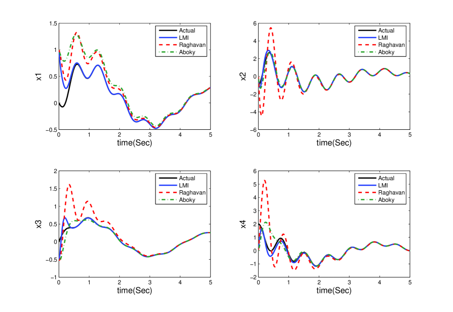
Figure 1: The true and estimated states of Example 2

Example 3. In this example we show the usage of of the multiobjective optimization of Theorem 5 in the design of $H_{\infty}$ observers. Consider the following system

$$x = \left[\begin{array}[]{cc}x_{1}&x_{2}\\ \end{array}\right]^{T}$$ (132)

$$\dot{x} = \left[\begin{array}[]{cc}0&1\\ -1&-1\\ \end{array}\right]x+\left[\begin{array}[]{c}x_{1}^{3}\\ -6x_{1}^{5}-6x_{1}^{2}x_{2}-2x_{1}^{4}-2x_{1}^{2}\\ \end{array}\right]$$ (137)

$$y = \left[\begin{array}[]{cc}1&0\end{array}\right]x.$$ (139)

The systems is locally Lipschitz. Its Lipschitz constant is region-based. Suppose we consider the region $\mathcal{D}$ as follows

$$\mathcal{D} = \biggl{\{}(x_{1},x_{2})\in\mathbb{R}^{2}\ |\ x_{1}\leq 0.25\biggr{\}}$$

in which the Lipschitz constant is $\gamma=0.4167$. We choose

$$H =0.5I$$

$$B =\left[\begin{array}[]{cc}1&1\\ \end{array}\right]^{T}$$ (141)

$$D =0.2$$

$$\beta =0.05$$

and solve the multiobjective optimization problem of Theorem 5 with $\lambda=0.9$. We get

$$\gamma^{*} =0.5525$$

$$\mu^{*} =1.1705$$

$$\alpha =1.6260$$

$$\epsilon =2.2435\times 10^{-4}$$

$$L =\left[\begin{array}[]{cc}23.7025&13.7272\\ \end{array}\right]^{T}.$$ (143)

The true and estimated values of states are shown in Figure 2. We have assumed that

$$x(0) = \left[\begin{array}[]{cc}-0.2&-1.45\end{array}\right]^{T}$$ (145)

$$\hat{x}(0) = \left[\begin{array}[]{cc}0.25&-2\end{array}\right]^{T}$$ (147)

$$w(t) = 0.15\exp(-t)\sin(t).$$

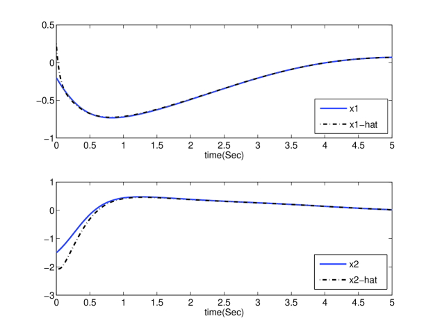
Figure 2: The true and estimated states of Example 3 in the presence of disturbance

The values of $\gamma^{*}$, $\mu^{*}$, norm of the observer gain matrix, $\bar{\sigma}(L)$, and the optimal trade-off curve between $\gamma^{*}$ and $\mu^{*}$ over the range of $\lambda$ when the decay rate is fixed ($\beta=0.05$) are shown in Figure 3.

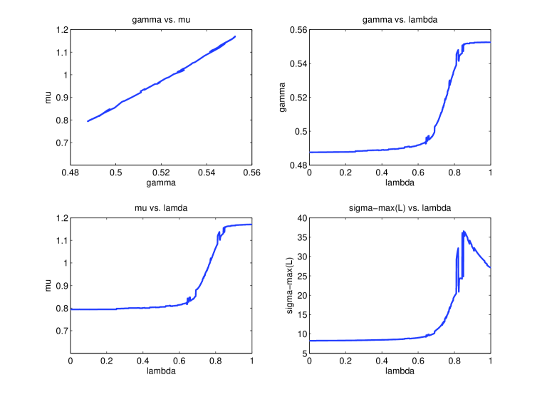
Figure 3: $\gamma^{*}$, $\mu^{*}$ and $\bar{\sigma}(L)$, and the optimal trade-off curve with $\beta=0.05$

The optimal surfaces of $\gamma^{*}$ and $\mu^{*}$ over the range of $\lambda$ when the decay rate is variable are shown in Figures 4 and 5, respectively.

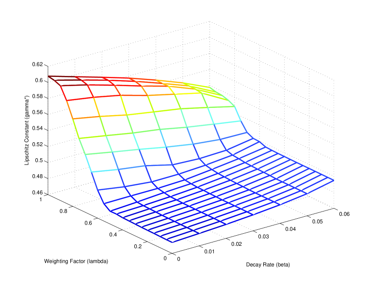
Figure 4: The optimal surface of $\gamma^{*}$

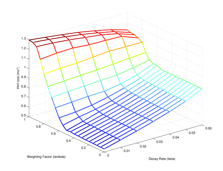
Figure 5: The optimal surface of $\mu^{*}$

7 Conclusions

A new method of robust observer design for Lipschitz nonlinear systems proposed based on LMI optimization. The Lipschitz constant of the nonlinear system can be maximized so that the observer error dynamics not only be asymptotically stable but also the observer can tolerate some additive nonlinear uncertainty. In addition, the result extended to a robust $H_{\infty}$ nonlinear observer. The obtained observer has three features, simultaneously. Asymptotic stability, robustness against nonlinear uncertainty and minimized guaranteed $H_{\infty}$ cost. Thanks to the linearity of the proposed LMIs in both admissible Lipschitz constant and the disturbance attenuation level, they can be simultaneously optimized through convex multiobjective optimization. The observer high performance showed through design examples.

References

- [1] F. Thau, “Observing the state of nonlinear dynamic systems,” International Journal of Control, vol. 17, no. 3, pp. 471–479, 1973.
- [2] S. Raghavan and J. Hedrick, “Observer design for a class of nonlinear systems,” International Journal of Control, vol. 59, no. 2, pp. 515 – 528, 1994.
- [3] R. Rajamani, “Observers for Lipschitz nonlinear systems,” IEEE Transactions on Automatic Control, vol. 43, no. 3, pp. 397 – 401, 1998.
- [4] R. Rajamani and Y. M. Cho, “Existence and design of observers for nonlinear systems: Relation to distance to unobservability,” International Journal of Control, vol. 69, no. 5, pp. 717–731, 1998.
- [5] C. Aboky, G. Sallet, and I. C. Walda, “Observers for Lipschitz non-linear systems,” International Journal of Control, vol. 75, no. 3, pp. 534–537, 2002.
- [6] A. M. Pertew, H. Marquez, and Q. Zhao, “Dynamic observers for nonlinear Lipschitz systems.” Proceedings of 16th IFAC World Congress, Prague, Czech Republic, 2005.
- [7] A. Howell and J. K. Hedrick, “Nonlinear observer design via convex optimization,” Proceedings of the American Control Conference, vol. 3, pp. 2088–2093, 2002.
- [8] S. Boyd, L. E. Ghaoui, E. Feron, and V. Balakrishnan, Linear matrix inequalities in system and control theory. SIAM, PA, 1994.
- [9] C. E. de Souza, L. Xie, and Y. Wang, “ filtering for a class of uncertain nonlinear systems,” Systems and Control Letters, vol. 20, no. 6, pp. 419–426, 1993.
- [10] Y. Wang, L. Xie, and C. E. de Souza, “Robust control of a class of uncertain nonlinear systems,” Systems and Control Letters, vol. 19, no. 2, pp. 139–149, 1992.
- [11] H. Khalil, Nonlinear Control Systems, Third Edition. Prentice Hall, N.J., 2002.
- [12] H. J. Marquez, Nonlinear Control Systems: Analysis and Design. Wiley, NY, 2003.
- [13] G. Wood and P. Zhang, “Estimation of the lipschitz constant of a function,” Journal of Global Optimization, vol. 8, no. 1, pp. 91–103, 1996.
- [14] S. Xu, “Robust filtering for a class of discrete-time uncertain nonlinear systems with state delay,” IEEE Transactions on Circuits and Systems I: Fundamental Theory and Applications, vol. 49, no. 12, pp. 1853 – 1859, 2002.
- [15] F. Zhu and Z. Han, “A note on observers for Lipschitz nonlinear systems,” IEEE Transactions on Automatic Control, vol. 47, no. 10, pp. 1751–1754, 2002.
- [16] S. Boyd and L. Vandenberghe, Convex Optimization. Cambrige University Press, 2004.