Statistical inference optimized with respect to the observed sample for single or multiple comparisons

Abstract

The normalized maximum likelihood (NML) is a recent penalized likelihood that has properties that justify defining the amount of discrimination information (DI) in the data supporting an alternative hypothesis over a null hypothesis as the logarithm of an NML ratio, namely, the alternative hypothesis NML divided by the null hypothesis NML. The resulting DI, like the Bayes factor but unlike the p-value, measures the strength of evidence for an alternative hypothesis over a null hypothesis such that the probability of misleading evidence vanishes asymptotically under weak regularity conditions and such that evidence can support a simple null hypothesis. Unlike the Bayes factor, the DI does not require a prior distribution and is minimax optimal in a sense that does not involve averaging over outcomes that did not occur. Replacing a (possibly pseudo-) likelihood function with its weighted counterpart extends the scope of the DI to models for which the unweighted NML is undefined. The likelihood weights leverage side information, either in data associated with comparisons other than the comparison at hand or in the parameter value of a simple null hypothesis. Two case studies, one involving multiple populations and the other involving multiple biological features, indicate that the DI is robust to the type of side information used when that information is assigned the weight of a single observation. Such robustness suggests that very little adjustment for multiple comparisons is warranted if the sample size is at least moderate.

David R. Bickel
Ottawa Institute of Systems Biology
Department of Biochemistry, Microbiology, and Immunology
Department of Mathematics and Statistics
University of Ottawa
451 Smyth Road
Ottawa, Ontario, K1H 8M5

Keywords: indirect information; information criteria; information for discrimination; minimum description length; model selection; multiple comparison procedure; multiple testing; normalized maximum likelihood; penalized likelihood; reduced likelihood; weighted likelihood

1 Introduction

1.1 Quantifying statistical evidence

Many areas of science involve investigations of whether some effect is present and thus call for statistical methods that assess the evidence pertaining to whether a null hypothesis or an alternative hypothesis is closer to the system studied. For example, many experimental biologists are more interested in whether gene expression levels differ between control and treatment groups than in the effect size itself.

Because not all samples are representative of their populations, the amount of evidence against the null hypothesis is misleadingly high for some samples. Although the probability of observing such an unrepresentative sample should decrease as the size of the sample increases, that is not the case if proximity of a p-value to 0 is interpreted as the strength of evidence against the null hypothesis. Indeed, the distribution of the p-value associated with a simple (point) null hypothesis remains the same at all sample sizes if the null hypothesis holds, making the p-value impossible to interpret as a level of evidence apart from considering the sample size, as Royall (1997), Blume and Peipert (2003), and others have argued; cf. Efron and Gous (2001) on the sample-size incoherence of significance testing. Bickel (2010c) defined the lacking property by calling a measure of evidence interpretable if its probability of misleading evidence vanishes asymptotically. That is, a measure of evidence satisfies the interpretability condition only if the frequentist probability of observing a sample that has misleading evidence exceeding some fixed threshold converges to 0 as the sample size diverges.

Another adverse consequence of treating the p-value as a measure of evidence is its inability to indicate evidence in favor of a simple null hypothesis. In general, the amount of information in the data that favors a simple null hypothesis cannot be quantified by the p-value since it can only indicate whether there is evidence against it.

The Bayes factor in principle overcomes the above limitations of the p-value but poses the notorious problem of specifying the prior distribution of a nuisance parameter that is not random in the frequentist sense. Any solution to the problem has practical implications since the Bayes factor is sensitive to prior specification (Kass and Raftery, 1995).

Subjective prior distributions have the advantage of coherence and yet are rarely used in data analysis since they depend on arbitrary choices in prior specification. On the other hand, the improper prior distributions generated by conventional algorithms cannot be directly applied to model selection since they would leave the Bayes factor undefined. That has been overcome to some extent by dividing the data into training and test samples, with the training samples generating proper priors for use with test samples, but at the expense of requiring the specification of training samples and, in the presence of multiple training samples, a method of averaging (Berger and Pericchi, 1996). Further, the interpretation of the resulting posterior probability is not clear except perhaps as an approximation to an agent’s level of belief (Bernardo, 1997).

1.2 Repeated-sampling optimality

Since there are many potential measures of evidence, most notably the Bayes factors defined by different priors, that satisfy the criteria that a measure of evidence be interpretable and that it can support a simple null hypothesis, an optimality criterion will be applied to determine a unique method of hypothesis testing and more general model selection. Before doing so, that criterion will be distinguished from standards of optimality in the received framework of statistics, that of Neyman and Pearson as generalized by Wald.

The goal of minimizing risk, the expected loss with respect to a sampling distribution (Wald, 1961), has provided a unified framework of estimation and testing and, as briefly reviewed in Bickel (2010a, §3.1), has led to recent multiple comparison procedures. However, Fraser and Reid (1990), Fraser (2004), Sprott (2004), and other frequentist statisticians have criticized the framework for promoting opportunistic trade-offs between hypothetical samples, thereby potentially misleading scientists and yielding unacceptably pathological procedures. The main non-Bayesian alternative involves replacing the marginal sampling distribution with a conditional sampling distribution given an exact or approximate ancillary statistic (e.g., Sprott, 2000, §3.3).

While conditioning on an ancillary statistic makes the reference distribution more relevant to inference on the basis of the observed sample (Fisher, 1973), it still does not permit statements about the actual loss incurred. For example, the confidence level remains the proportion of confidence intervals corresponding to repeated samples that cover the parameter of interest. Although the use of exact confidence intervals minimizes a risk (Cornfield, 1969; Bickel, 2009), it is silent regarding the loss associated with the observed sample.

1.3 Observed-sample optimality

1.3.1 Information-theoretic inference

In order to address the issues outlined above, this paper continues the development of a new information-theoretic alternative to previous approaches to statistical inference. The concept of a predictive distribution will enable defining minimax optimality without repeated-sampling or posterior-distribution averages. This approach is presented here largely without the terminology of its origin in universal source coding (Shtarkov, 1987).

Consider the observed data vector $x\in\mathcal{X}^{n}$. Let $\mathcal{E}\left(\Omega\right)$ denote the set of all probability density functions on any sample space $\Omega$, and let $\mathcal{F}=\left\{f_{\phi}:\phi\in\Phi\right\}\subset\mathcal{E}\left(\mathcal{X}^{n}\right)$ denote a parametric family of density functions on $\mathcal{X}^{n}$ for parameter space $\Phi$. (Herein, the probability densities are Radon-Nikodym derivatives, reducing to probability masses if $\mathcal{X}$ is countable.) The maximum likelihood estimate of $\phi$, denoted by $\hat{\phi}\left(x\right)$, is assumed to be unique.

The regret of a predictive density $\bar{f}\in\mathcal{E}\left(\mathcal{X}^{n}\right)$ is the logarithmic loss

$$\operatorname{reg}\left(\bar{f},x;\Phi\right) = -\log\bar{f}\left(x\right)-\inf_{\phi\in\Phi}\left(-\log f_{\phi}\left(x\right)\right)=\log\frac{f_{\hat{\phi}\left(x\right)}\left(x\right)}{\bar{f}\left(x\right)}$$ (1)

for any $x\in\mathcal{X}^{n}$. The $\mathcal{E}\left(\mathcal{X}^{n}\right)$-optimal predictive density function relative to $\mathcal{F}$,

$$\bar{f}_{0}=\arg\inf_{\bar{f}\in\mathcal{E}\left(\mathcal{X}^{n}\right)}\sup_{u\in\mathcal{X}^{n}}\operatorname{reg}\left(\bar{f},u;\Phi\right),$$ (2)

while by definition in $\mathcal{E}\left(\mathcal{X}^{n}\right)$, is not necessarily in $\mathcal{F}$. Rather, $\bar{f}_{0}$ is a probability density function that represents the entire family $\mathcal{F}$ with a single distribution, much as does a prior predictive density function. Instead of averaging the members of $\mathcal{F}$ with respect to a prior distribution, the present definition employs $\mathcal{F}$ in equation (2) for each $u\in\mathcal{X}^{n}$ through the maximization of the likelihood over $\phi\in\Phi$, as seen by substituting $u$ for $x$ in equation (1).

Originally motivated in the information theory literature by a need to minimize codelength (Shtarkov, 1987), equation (2) defines the type of minimax optimality employed as opposed to the optimality of Section 1.2. (According to the minimum description length principle, each family of distributions corresponds to an algorithm of most efficiently encoding the information in $x$ (Rissanen, 2007; Grünwald, 2007; Rissanen, 2009).) The predictive density function $\bar{f}_{0}$ is optimal in that it solves the minimax problem involving all $u\in\mathcal{X}^{n}$, and thus for the observed sample $x\in\mathcal{X}^{n}$, rather than the more usual minimax problem involving an expectation value over all samples, as in the standard decision theory of frequentism. The following result (Shtarkov, 1987; Rissanen, 2007; Grünwald, 2007), to be proved in Section 2.2.1 for a more general optimization problem, sheds light on the nature of the optimality considered.

Theorem 1.

If $\int_{\mathcal{X}^{n}}f_{\hat{\phi}\left(u\right)}\left(u\right)du<\infty$, then the $\mathcal{E}\left(\mathcal{X}^{n}\right)$-optimal predictive density function relative to $\mathcal{F}$ is

$$\bar{f}_{0}\left(\bullet\right)=\bar{f}_{0}\left(\bullet;\Phi\right)=\frac{f_{\hat{\phi}\left(\bullet\right)}\left(\bullet\right)}{\int_{\mathcal{X}^{n}}f_{\hat{\phi}\left(u\right)}\left(u\right)du}.$$ (3)

Proof.

This proof by contradiction is based on the direct proof given by Grünwald (2007, §6.2.1). Assume, contrary to the claim, that the density function $\bar{f}_{0}$ that satisfies equation (3) is not the optimal predictive density function. Since, for any $v\in\mathcal{X}^{n}$, the ratio $\bar{f}_{0}\left(v\right)/f_{\hat{\phi}\left(v\right)}\left(v\right)$ does not depend on $v$, it follows that, for any $\breve{f}\in\mathcal{E}\left(\mathcal{X}^{n}\right)\backslash\left\{\bar{f}_{0}\right\}$, there is a $v\in\mathcal{X}^{n}$ such that $\breve{f}\left(v\right)/f_{\hat{\phi}\left(v\right)}\left(v\right)<\bar{f}_{0}\left(v\right)/f_{\hat{\phi}\left(v\right)}\left(v\right)$. Therefore, given any $\breve{f}\in\mathcal{E}\left(\mathcal{X}^{n}\right)\backslash\left\{\bar{f}_{0}\right\}$, there is a $v\in\mathcal{X}^{n}$ such that $\operatorname{reg}\left(\bar{f}_{0},v;\Phi\right)<\operatorname{reg}\left(\breve{f},v;\Phi\right)$, which contradicts the assumption. ∎

Note that $u$, the dummy variable of integration over $\mathcal{X}^{n}$, appears twice in the integrand. For the observed $x\in\mathcal{X}^{n}$, the quantity $\bar{f}_{0}\left(x\right)=\bar{f}_{0}\left(x;\Phi\right)$ is called the normalized maximum likelihood (NML) with respect to $\Phi$.

According to Theorem 1, the minimax optimality (2) of $\bar{f}_{0}$ guarantees that $\operatorname{reg}\left(\bar{f}_{0},x;\Phi\right)$, the regret due to the observed sample, cannot exceed $\sup_{u\in\mathcal{X}^{n}}\operatorname{reg}\left(\bar{f}_{0},u;\Phi\right)$, the regret due to the worst-case sample. In that sense, $\bar{f}_{0}$ is optimal for the observed sample. By contrast, standard frequentist optimality, concerned only with loss averaged over all possible samples, guarantees no bound on the loss inflicted by any individual sample.

Such observed-sample optimality justifies selecting the model or hypothesis corresponding to the family $\mathcal{F}_{i}$ of distributions that minimizes $-\log\bar{f}_{0}\left(x;\Phi_{i}\right)$, the observed prediction error of the $i$th among a finite number of distribution families under consideration. Following the terminology of Kullback (1968) and Bickel (2010b), $-\log\bar{f}_{0}\left(x;\left\{\phi_{0}\right\}\right)-\left(-\log\bar{f}_{0}\left(x;\Phi\right)\right)$ would be the information in $x$ for discrimination in favor of the alternative hypothesis that $\phi\neq\phi_{0}$ over the null hypothesis that $\phi=\phi_{0}$. Such information is an interpretable measure of evidence under general conditions and can quantify the strength of any evidence in favor of the null hypothesis as well as that of any evidence against it. More importantly, the information for discrimination optimally quantifies the difference in how well each model or hypothesis predicts relative to ideal predictors of individual samples rather than relative to unknown true distributions, the ideal predictors in the sense of averages over samples. The Kullback-Leibler risk, for example, only measures mean discrimination information relative to unknown ideal predictors in the average sense.

Since the base of the logarithm is inconsequential, it may be chosen for convenience of interpretation. The binary logarithm $\left(\log_{2}\right)$, yielding the number of bits of information, enables not only immediate exponentiation back to the ratio domain but also the use of grades of evidence that are both broad enough and refined enough for applications across scientific disciplines (Table 1). Except for the distinction between negligible and weak evidence, the grades closely mirror those Jeffreys (1948) originally proposed for the Bayes factor; cf. Bickel (2010c). Accordingly, the $\left[3,5\right)$ grade of Table 1 is what Royall (1997, §1.12) considers “fairly strong evidence” for one simple hypothesis over another, and the $\left[5,7\right)$ and $\left[7,\infty\right)$ grades together constitute his “quite strong evidence.”

Information (bits)	$\left(0,1\right)$	$\left[1,2\right)$	$\left[2,3\right)$	$\left[3,5\right)$	$\left[5,7\right)$	$\left[7,\infty\right)$
Evidence grade	Negligible	Weak	Moderate	Strong	Very strong	Overwhelming

Table 1: Heuristic grades of evidence for an alternative hypothesis over a null hypothesis corresponding to intervals of the information for discrimination. The absolute value of a negative amount of information gives the grade of evidence favoring the null hypothesis.

1.3.2 Extension of information-theoretic inference

Despite the unique observed-sample optimality of the NML for quantifying discrimination information, three shortcomings make it impractical for use in many biostatistics applications. First, since such applications typically partition $\phi$ into an interest parameter $\theta$ and a nuisance parameter $\lambda$, the regret is relative to an ideal distribution determined by maximizing the likelihood not only over $\theta$ but also over $\lambda$. As a result, the ideal member of the family of distributions would be considered a better predictor than another member that has the same value of $\theta$ on the basis of having a different value of $\lambda$, which should be irrelevant. Thus, the NML is inadequate for testing hypotheses about $\theta$ in the presence of $\lambda$.

Second, the NML only uses information that is in $x$, but considering such information about the parameter in isolation from other available information can be misleading unless the sample size is sufficiently large. Additional information may be available in data from other populations, from other biological features such as genes or SNPs, or from other feature-feature comparisons. Even in the absence of such incidental information, there would be some information in the fact that the null hypothesis that $\phi=\phi_{0}$ is seriously considered.

Third, the normalizing denominator of equation (3), the logarithm of which is called the parametric complexity of $\mathcal{F}$, is infinite for typical families of distributions, including the normal family. Each of the variant NMLs proposed to address the problem introduces its own conceptual difficulties (Lanterman, 2005; Grünwald, 2007). For example, Rissanen (2007, §5.2.4), Rissanen and Roos (2007), and Grünwald (2007, §11.4.2) proposed conditional versions of the NML. Cf. related work by Takimoto and Warmuth (2000).

To overcome the first of the three identified problems with NML, it is generalized in Section 2 by replacing the original data with a statistic that is a function of the data and that has a distribution depending on $\theta$ but not on $\lambda$. Since the information in the data relevant to the interest parameter is largely confined to the statistic, that information can be better quantified in terms of the distribution of the statistic than in terms of the distribution of the original data, the latter depending on the value of the nuisance parameter. In terms of the minimum description length (MDL) metaphor (Rissanen, 2007; Grünwald, 2007), the data are first compressed with little information loss by reduction to a smaller-dimensional statistic and then further compressed by the family of distributions.

The use of a weighted likelihood addresses the second problem in the same section, which also includes some results relevant to the probability of observing misleading information. (The weighted likelihood was originally proposed for bias-variance trade-offs given relatively small $n_{i}$ but potentially large $N$ (Feifang, 2002). More formally, Wang and Zidek (2005) derived the weighted likelihood from the minimization of Kullback-Leibler loss.)

As a by-product for commonly used distribution families, that solution to the second problem automatically solves the third problem, as illustrated in Section 3 with a multiple-population data set and a multiple-feature data set. Finally, Section 4 concludes by highlighting desirable properties of the new NML-based measure of information for discrimination.

2 Optimal inference

2.1 Preliminaries

2.1.1 Weighted likelihood

The framework of Section 1.3 is generalized by the use of data reduction to eliminate a nuisance parameter in $\phi$. Consider a measurable map $\tau_{n}:\mathcal{X}^{n}\rightarrow\mathcal{T}\left(n\right)$. Let $\theta:\Phi\rightarrow\Theta$ denote a subparameter function such that the probability density of $\tau_{n}\left(X\right)$ is $g_{\theta\left(\phi\right)}\left(\tau_{n}\left(X\right)\right)$, abbreviated as $g_{\theta}\left(\tau\left(X\right)\right)$; the dependence of the density function $g_{\theta}$ on $n$ is suppressed. Thus, the reduction of the data $X$ to a statistic $\tau\left(X\right)$ has the effect of replacing the full parameter $\phi$ with the interest parameter $\theta$. Important special cases of $L\left(\theta;\tau\left(x\right)\right)=g_{\theta}\left(\tau\left(x\right)\right)$ as a function of $\theta$ are conditional likelihood functions and marginal likelihood functions (Royall, 1997; Severini, 2000; Bickel, 2010b).

The framework is now extended to $N$ hypotheses or comparisons. Let $\mathcal{G}_{n,i}=\left\{g_{n,i,\theta}:\theta\in\Theta\right\}\subset\mathcal{E}\left(\mathcal{T}\left(n\right)\right)$ denote the parametric family of density functions on $\mathcal{T}\left(n\right)$ for parameter space $\Theta$. The “$n$” and “$i$” subscripts will be dropped when their values are clear. For the $i$th of $N$ null hypotheses or comparisons, suppose $x_{i}\in\mathcal{X}^{n_{i}}$ is a realization of the random vector $X_{i}$ of $n_{i}$ independent components. Then each $T_{i}=\tau\left(X_{i}\right)$ is distributed with density $g_{\theta_{i}}=g_{n_{i},i,\theta_{i}}$, and each outcome $t_{i}=\tau\left(x_{i}\right)$ is an element of $\mathcal{T}_{i}=\mathcal{T}\left(n_{i}\right)$. Let $L_{i}\left(\theta;\tau\left(x_{i}\right)\right)=g_{n,i,\theta}\left(\tau\left(x_{i}\right)\right)=g_{\theta}\left(\tau\left(x_{i}\right)\right)$, giving each comparison its own likelihood function.

Mapping $\mathcal{X}^{n_{i}}$ to $\mathcal{T}_{i}=\mathbb{R}^{D}$ is common in data reduction applications in which $\Theta=\mathbb{R}^{D}$. Assigning a common parametric family to all comparisons ($\mathcal{G}_{n,i}=\mathcal{G}_{n,1}$ for all $i$) is usually appropriate when each comparison corresponds to a biological feature, as in Section 3.2.

The observation $\mathbf{x}=\left\langle x_{1},\dots,x_{N}\right\rangle$ generates the test statistic vector $\mathbf{t}=\left\langle t_{1},\dots,t_{N}\right\rangle=\left\langle\tau\left(x_{1}\right),\dots,\tau\left(x_{N}\right)\right\rangle$, an outcome of $\mathbf{T}=\left\langle T_{1},\dots,T_{N}\right\rangle=\left\langle\tau\left(X_{1}\right),\dots,\tau\left(X_{N}\right)\right\rangle$. For inference about $\theta_{i}$ on the basis of $\mathbf{t}$, the weighted likelihood function $\bar{L}_{i}\left(\bullet;\mathbf{t}\right):\Theta\rightarrow\left[0,\infty\right)$ is defined by

$$\log\bar{L}_{i}\left(\theta_{i};\mathbf{t}\right)=\sum_{j=1}^{N}w_{ij}\log L_{j}\left(\theta_{i};t_{j}\right),$$ (4)

where the weights $w_{i}=\left\langle w_{i1},\dots,w_{iN}\right\rangle$ are real numbers that may depend on $\left\langle n_{1},\dots,n_{N}\right\rangle$ and that satisfy $w_{ii}\geq w_{ij}$ (Feifang, 2002). The weights normally also conform to $\sum_{j=1}^{N}w_{ij}=1$, a requirement that will be temporarily relaxed in Section 2.2.1.

Example 2.

In most microarray studies, the expression levels of $N$ genes are measured with the goal of determining which genes are differentially expressed between a treatment/perturbation group of $m$ replicates and a control group of $n$ replicates; each of these biological replicates represents one or more organisms. (Single-channel arrays do not require the pairing of replicates between groups as did the dual-channel arrays.) Following the typical assumption that intensity values are lognormally distributed, let $x_{i}=\left\langle x_{i1},\dots,x_{im}\right\rangle$ and $y_{i}=\left\langle y_{i1},\dots,y_{in}\right\rangle$ denote the logarithms of the $m$ and $n$ intensities of the $i$th gene in the perturbation and control group, respectively. For small numbers of replicates, the assumption of a common variance within each group is useful: $X_{ij}\sim\operatorname{N}\left(\xi_{i},\sigma_{i}^{2}\right)$ and $Y_{ij}\sim\operatorname{N}\left(\eta_{i},\sigma_{i}^{2}\right)$ with realized values $X_{ij}=x_{ij}$ for $j=1,\dots,m$ and $Y_{ij}=y_{ij}$ for $j=1,\dots,n$. If $\theta_{i}$ is the absolute value of the inverse coefficient of variation $\left(\xi_{i}-\eta_{i}\right)/\sigma_{i}$, then $t_{i}$ is conveniently taken as the absolute value of the two-sample, equal-variance $t$-statistic, which has a noncentral $t$ distribution with noncentrality parameter $\left(m^{-1}+n^{-1}\right)^{-1/2}\theta_{i}$ and $m+n-2$ degrees of freedom.

The sampling distribution of $\mathbf{T}$ is denoted by $P$ to specify properties of the weights while accommodating model misspecification, the case that there is not a $\theta_{i}\in\Theta$ such that $g_{\theta_{i}}$ is a density admitted by the marginal distribution $P\left(T_{i}\in\bullet\right)$ for all $i\in\left\{1,\dots,N\right\}$. With suitable weights and the assumption that $\hat{\theta}_{i}\left(\mathbf{T}\right)=\arg\sup_{\theta\in\Theta}\bar{L}_{i}\left(\theta;\mathbf{T}\right)$ is almost surely unique for all $i\in\left\{1,\dots,N\right\}$, the difference between $\hat{\theta}_{i}\left(\mathbf{T}\right)$ and the conventional maximum likelihood estimator of $\theta_{i}$ almost surely converges to 0 as $n_{i}$ diverges with $N$ held fixed. Specifically, $w_{ii}=1+o_{P}\left(1\right)$ and $i\neq j\implies w_{ij}=o_{P}\left(1\right)$ ensure that $\hat{\theta}_{i}\left(\mathbf{T}\right)=\arg\sup_{\theta\in\Theta}L\left(\theta;x_{i}\right)+o_{P}\left(1\right)$, where the term $o_{P}\left(1\right)$ converges to 0 with $P$-probability 1 as $n_{i}\rightarrow\infty$ with any ratio $n_{j}/n_{k}$ bounded by constants: $n_{j}=O\left(n_{k}\right)$ for all $j,k\in\left\{1,\dots,N\right\}$.

2.1.2 Predictive loss

For some $\bar{g}\in\mathcal{E}\left(\mathcal{T}_{i}\right)$, the generalized regret

$$\operatorname{reg}_{i}\left(\bar{g},\mathbf{t};\Theta\right)=-\log\bar{g}\left(\tau\left(x_{i}\right)\right)-\inf_{\theta\in\Theta}\left(-\log\bar{L}_{i}\left(\theta;\mathbf{t}\right)\right)=\log\frac{\bar{L}_{i}\left(\hat{\theta}_{i}\left(\mathbf{t}\right);\mathbf{t}\right)}{\bar{g}\left(\tau\left(x_{i}\right)\right)}$$ (5)

measures loss incurred by the likelihood associated with $\bar{g}$, the predictive distribution, relative to $\bar{L}_{i}\left(\hat{\theta}_{i}\left(\mathbf{t}\right);\mathbf{t}\right)$, the maximum weighted likelihood of $\theta_{i}$. In other words, $\operatorname{reg}_{i}\left(\bar{g},\mathbf{t};\Theta\right)$ is the discrepancy between error in predicting the value of $\tau\left(x\right)$ on the basis of $\bar{g}$ and the prediction error minimized over the interest parameter. The latter error is more relevant to hypotheses about the value of $\theta$ than a prediction error minimized over the full parameter $\phi$, including the nuisance parameter $\lambda$ (§1.3). Thus, $\operatorname{reg}_{i}\left(\bar{g},\mathbf{t};\Theta\right)$ replaces $\operatorname{reg}\left(\bar{f},x;\Phi\right)$ as the regret in the presence of the nuisance parameter or a nonzero weight other than $w_{ii}$.

2.2 Optimal predictive distribution

2.2.1 Exact predictive distribution

For each $t\in\mathcal{T}_{i}$, let $\mathbf{t}_{i}\left(t\right)$ denote the $N$-tuple of statistics that is equal to $\mathbf{t}$ in all components except the $i$th, which has $t$ in place of $t_{i}$. For example, $\mathbf{t}_{1}\left(t\right)=\left\langle t,t_{2},\dots,t_{N}\right\rangle$, but $\mathbf{t}_{i}\left(t\right)=\left\langle t_{1},\dots,t_{i-1},t,t_{i+1},\dots,t_{N}\right\rangle$ if $3\leq i\leq N-2$.

The optimal predictive density function of Section 1.3 is a special case of

$$\bar{g}_{i}=\arg\inf_{\bar{g}\in\mathcal{E}\left(\mathcal{T}_{i}\right)}\sup_{t\in\mathcal{T}_{i}}\operatorname{reg}_{i}\left(\bar{g},\mathbf{t}_{i}\left(t\right);\Theta\right),$$

the $\mathcal{E}\left(\mathcal{T}_{i}\right)$-optimal predictive density function relative to $\left\langle\mathcal{G},w_{i}\right\rangle$.

Theorem 3.

Given some $i\in\left\{1,\dots,N\right\}$ and $\mathbf{t}\in\mathcal{T}_{1}\times\cdots\times\mathcal{T}_{N}$, if $\int\bar{L}_{i}\left(\hat{\theta}_{i}\left(\mathbf{t}_{i}\left(t\right)\right);\mathbf{t}_{i}\left(t\right)\right)dt<\infty$, then, for all $t_{i}\in\mathcal{T}_{i}$, the $\mathcal{E}\left(\mathcal{T}_{i}\right)$-optimal predictive density function relative to $\left\langle\mathcal{G},w_{i}\right\rangle$ satisfies

$$\bar{g}_{i}\left(t_{i}\right)=\frac{\bar{L}_{i}\left(\hat{\theta}_{i}\left(\mathbf{t}\right);\mathbf{t}\right)}{\int_{\mathcal{T}_{i}}\bar{L}_{i}\left(\hat{\theta}_{i}\left(\mathbf{t}_{i}\left(t\right)\right);\mathbf{t}_{i}\left(t\right)\right)dt}.$$ (6)

Proof.

The present argument follows that used to prove Theorem 1. Assume, contrary to the claim, that the density function $\bar{g}_{i}$ that satisfies equation (6) for all $t_{i}\in\mathcal{T}_{i}$ is not the optimal predictive density function relative to $\left\langle\mathcal{G},w_{i}\right\rangle$. The substitution $\bar{L}_{i}\left(\hat{\theta}_{i}\left(\mathbf{t}\right);\mathbf{t}\right)=\bar{L}_{i}\left(\hat{\theta}_{i}\left(\mathbf{t}_{i}\left(t_{i}\right)\right);\mathbf{t}_{i}\left(t_{i}\right)\right)$ demonstrates that the ratio $\bar{g}_{i}\left(t_{i}\right)/\bar{L}_{i}\left(\hat{\theta}_{i}\left(\mathbf{t}_{i}\left(t_{i}\right)\right);\mathbf{t}_{i}\left(t_{i}\right)\right)$ does not depend on $t_{i}$. It follows that, for any $\breve{g}_{i}\in\mathcal{E}\left(\mathcal{T}_{i}\right)\backslash\left\{\bar{g}_{i}\right\}$, there is a $t_{i}\in\mathcal{T}_{i}$ such that $\breve{g}_{i}\left(t_{i}\right)/\bar{L}_{i}\left(\hat{\theta}_{i}\left(\mathbf{t}_{i}\left(t_{i}\right)\right);\mathbf{t}_{i}\left(t_{i}\right)\right)<\bar{g}_{i}\left(t_{i}\right)/\bar{L}_{i}\left(\hat{\theta}_{i}\left(\mathbf{t}_{i}\left(t_{i}\right)\right);\mathbf{t}_{i}\left(t_{i}\right)\right)$. Therefore, given any $\breve{g}_{i}\in\mathcal{E}\left(\mathcal{T}_{i}\right)\backslash\left\{\bar{g}_{i}\right\}$, there is a $t_{i}\in\mathcal{T}_{i}$ such that $\operatorname{reg}_{i}\left(\bar{g}_{i},\mathbf{t}_{i}\left(t_{i}\right);\Theta\right)<\operatorname{reg}_{i}\left(\breve{g}_{i},\mathbf{t}_{i}\left(t_{i}\right);\Theta\right)$, which contradicts the assumption. ∎

For any $x_{i}\in\mathcal{X}^{n}$, the quantity $\bar{g}_{i}\left(\tau\left(x_{i}\right)\right)=\bar{g}_{i}\left(\tau\left(x_{i}\right);\Theta\right)$ is the normalized maximum weighted likelihood (NMWL) with respect to $\Theta$ or, more precisely, with respect to $\left\langle\mathcal{G},w_{i}\right\rangle$.

Example 4.

When the constraint that $\sum_{j=1}^{N}w_{ij}=1$ is relaxed, NMWL generalizes various previous NMLs as follows. If $\tau\left(x_{1}\right)=x_{1}$ for some $x_{1}\in\mathcal{X}^{n_{1}}$ and if $N=1$, the NMWL reduces to the probability density $\bar{g}_{1}\left(x_{1}\right)$ with $w_{1,1}=1$ and thus to $\bar{f}_{0}\left(x\right)$, the NML of equation (3). For an observed vector $\left\langle y_{1},\dots,y_{n_{1}}\right\rangle\in\mathcal{X}^{n_{1}}$, assigning $N=2$, $\theta_{1}=\theta_{2}$, $t_{1}=\left\langle y_{1},\dots,y_{n_{1}-1}\right\rangle$, and $t_{2}=y_{n_{1}}$ demonstrates that the prominent conditional NMLs are NMWLs in the case of IID data. In particular, Grünwald (2007, §11.4.2) considered $\bar{g}_{1}\left(\left\langle t_{1},t_{2}\right\rangle\right)$ with $w_{1,1}=w_{1,2}=1$. Conversely, Rissanen (2007, §5.2.4) and Rissanen and Roos (2007) studied $\bar{g}_{2}\left(\left\langle t_{1},t_{2}\right\rangle\right)$ with $w_{2,1}=w_{2,2}=1$, thereby facilitating computation of the normalizing constant in equation (6) since the integration is only over a scalar. The main drawback of applying conditional NMLs to the IID setting is the arbitrary nature of choosing an observation $x_{2}$ to leave out since the observations are not ordered in time (Grünwald, 2007, §11.4.3). The same issue arises in Bayesian model selection when an improper prior is conditioned on a minimal training sample before computing the Bayes factor. A popular solution is to take geometric or arithmetic averages over all possible minimal training samples (Berger and Pericchi, 2004). Analogous approaches to IID applications of conditional NMLs would likewise depend on arbitrary choices of averages and of training sample sizes (§1.1).

2.2.2 Approximate predictive distribution

A computationally efficient approximation to the NMWL is available if:

1. The weight of any comparison in focus is equal to that of any other comparison when it is in focus, i.e., $w_{ii}=w_{1,1}$ for all $i$.

2. The weight of each comparison not in focus is equal to that of any other comparison not in focus, i.e., $w_{ij}=w_{1,2}$ for all $i\neq j$.

3. The sample sizes and sample spaces are equal, i.e., $n_{i}=n_{1}$ and $\mathcal{T}_{i}=\mathcal{T}_{1}$ for all $i$.

4. All comparisons share a single family, i.e., $\mathcal{G}_{n_{1},i}=\mathcal{G}_{n_{1},1}$ and $L_{1}=L_{i}$ for all $i$.

Under those equal weight conditions, there is an approximate weight $\tilde{w}_{N+1}$ such that $\tilde{w}_{N+1}=w_{ii}$ for all $i$ and an approximate weight $\tilde{w}_{j}$ such that $\tilde{w}_{j}=\left(N-1\right)N^{-1}w_{ij}$ for all $i$ and $j$ except $i=j$. Then $\sum_{j=1}^{N+1}\tilde{w}_{j}=N\tilde{w}_{1}+\tilde{w}_{N+1}=\left(N-1\right)w_{1,2}+w_{1,1}=1$.

For any $t\in\mathcal{T}_{1}$, let $\tilde{\mathbf{t}}\left(t\right)$ denote $\left\langle t_{1},\dots,t_{N},t\right\rangle\in\mathcal{T}_{1}^{N+1}$. For inference about $\theta_{i}$ on the basis of $\mathbf{t}$, the approximate weighted likelihood function $\tilde{L}\left(\bullet;\tilde{\mathbf{t}}\left(t\right)\right):\Theta\rightarrow\left[0,\infty\right)$ is defined by

$$\log\tilde{L}\left(\theta_{i};\tilde{\mathbf{t}}\left(t\right)\right) = \sum_{j=1}^{N}\tilde{w}_{j}\log L_{j}\left(\theta_{i};t_{j}\right)+\tilde{w}_{N+1}\log L_{j}\left(\theta_{i};t\right)$$

$$= \frac{1-w_{1,1}}{N}\sum_{j=1}^{N}\log L_{1}\left(\theta_{i};t_{j}\right)+w_{1,1}\log L_{1}\left(\theta_{i};t\right),$$

the second equality implied by the equal weight conditions. Let $\hat{\theta}\left(\tilde{\mathbf{t}}\left(t\right)\right)=\arg\sup_{\theta\in\Theta}\tilde{L}\left(\theta;\tilde{\mathbf{t}}\left(t\right)\right)$.

The following theorem indicates that the exact NMWL (6) is approximated by

$$\tilde{g}_{i}\left(t_{i}\right)=\frac{\bar{L}_{i}\left(\hat{\theta}_{i}\left(\mathbf{t}\right);\mathbf{t}\right)}{\int_{\mathcal{T}_{1}}\tilde{L}\left(\hat{\theta}\left(\tilde{\mathbf{t}}\left(t\right)\right);\tilde{\mathbf{t}}\left(t\right)\right)dt},$$

which may be quickly calculated even for large $N$ since the denominator, not depending on $i$, need only be computed once. In the theorem and its supporting lemmas, $\tilde{\mathbf{T}}\left(t\right)=\left\langle T_{1},\dots,T_{N},t\right\rangle$, and $\overset{\text{a.s.}}{\rightarrow}$ denotes almost sure convergence as $N$ increases with $n_{1}$ fixed.

Lemma 5.

If the equal weight conditions hold and if $T_{1},\dots,T_{N}$ are drawn independently from a mixture distribution, then, for all $\theta\in\Theta$ and $t\in\mathcal{T}_{i}$,

$$\log\tilde{L}\left(\theta;\tilde{\mathbf{T}}\left(t\right)\right)-\log\bar{L}_{i}\left(\theta;\mathbf{T}_{i}\left(t\right)\right)\overset{\text{a.s.}}{\rightarrow}0.$$ (7)

Proof.

According to the equal weight conditions,

$$\log\tilde{L}\left(\theta;\tilde{\mathbf{T}}\left(t\right)\right)-\log\bar{L}_{i}\left(\theta;\mathbf{T}_{i}\left(t\right)\right) =$$

$$\left(\frac{1-\tilde{w}_{N+1}}{N}\sum_{j=1}^{N}\log L_{1}\left(\theta;T_{j}\right)+\tilde{w}_{N+1}\log L_{1}\left(\theta;T_{i}\right)\right)-\left(\frac{1-w_{ii}}{N-1}\sum_{j\neq i;i=1}^{N}\log L_{1}\left(\theta;T_{j}\right)+w_{ii}\log L_{1}\left(\theta;T_{i}\right)\right)$$

$$=\left(1-\tilde{w}_{N+1}\right)\left(\frac{1}{N}\sum_{j=1}^{N}\log L_{1}\left(\theta;T_{j}\right)-\frac{1}{N-1}\sum_{j\neq i;i=1}^{N}\log L_{1}\left(\theta;T_{j}\right)\right).$$

The second factor almost surely vanishes by the law of large numbers.∎

Lemma 6.

Under the assumptions of Lemma 5, the stipulations that $\hat{\theta}\left(\tilde{\mathbf{T}}\left(t\right)\right)$ and $\hat{\theta}_{i}\left(\mathbf{T}_{i}\left(t\right)\right)$ are almost always unique for all $t\in\mathcal{T}_{i}$ and that $L_{1}\left(\bullet;T_{i}\right)$ is almost surely continuous on $\Theta$ for all $i=1,\dots,N$ imply that, for all $i=1,\dots,N$ and $t\in\mathcal{T}_{i}$, $\hat{\theta}\left(\tilde{\mathbf{T}}\left(t\right)\right)-\hat{\theta}_{i}\left(\mathbf{T}_{i}\left(t\right)\right)\overset{\text{a.s.}}{\rightarrow}0.$

Proof.

By Lemma 5, equation (7) holds for all $\theta\in\Theta$. Thus, since almost sure convergence is preserved under almost surely continuous transformations (Serfling, 1980, §1.7),
$\arg\sup_{\theta\in\Theta}\tilde{L}\left(\theta;\tilde{\mathbf{T}}\left(t\right)\right)-\arg\sup_{\theta\in\Theta}\bar{L}_{i}\left(\theta;\mathbf{T}\right)\overset{\text{a.s.}}{\rightarrow}0.$∎

Theorem 7.

Under the assumptions of Lemma 6, the difference between the approximate and exact parametric complexities almost surely vanishes:

$$\int_{\mathcal{T}_{1}}\tilde{L}\left(\hat{\theta}\left(\tilde{\mathbf{T}}\left(t\right)\right);\tilde{\mathbf{T}}\left(t\right)\right)dt-\int_{\mathcal{T}_{i}}\bar{L}_{i}\left(\hat{\theta}_{i}\left(\mathbf{T}_{i}\left(t\right)\right);\mathbf{T}_{i}\left(t\right)\right)dt\overset{\text{a.s.}}{\rightarrow}0.$$ (8)

Proof.

Combining the results of Lemmas 5 and 6 gives

$$\tilde{L}\left(\hat{\theta}\left(\tilde{\mathbf{T}}\left(t\right)\right);\tilde{\mathbf{T}}\left(t\right)\right)-\bar{L}_{i}\left(\hat{\theta}_{i}\left(\mathbf{T}_{i}\left(t\right)\right);\mathbf{T}_{i}\left(t\right)\right)\overset{\text{a.s.}}{\rightarrow}0$$

for all $t\in\mathcal{T}_{i}$ since $\mathcal{T}_{i}=\mathcal{T}_{1}$ and the functions are almost surely continuous by assumption. ∎

2.3 Optimal discrimination information

For any $\Theta^{\prime}\subseteq\Theta$, let $\bar{g}_{i}\left(t_{i};\Theta^{\prime}\right)$ denote the optimal predictive density function relative to $\left\langle\left\{g_{\theta}:\theta\in\Theta^{\prime}\right\},w_{i}\right\rangle$ as defined in Section 2.2.1. For any $\Theta_{0},\Theta_{1}\subseteq\Theta$, the optimal information in $x$ for discrimination in favor of the hypothesis that $\theta_{i}\in\Theta_{1}$ over the hypothesis that $\theta_{i}\in\Theta_{0}$ is

$$\bar{I}_{i}\left(\Theta_{1},\Theta_{0}\right)=-\log\bar{g}_{i}\left(t_{i};\Theta_{0}\right)-\left(-\log\bar{g}_{i}\left(t_{i};\Theta_{1}\right)\right),$$

generalizing quantities in Kullback (1968), Rissanen (1987), Bickel (2010c), and Bickel (2010b). The approximate optimal information $\tilde{I}_{i}\left(\Theta_{1},\Theta_{0}\right)$ is defined identically except with $\tilde{g}_{i}$ in place of $\bar{g}_{i}$. $\bar{I}_{i}\left(\Theta_{1},\Theta_{0}\right)$ is not restricted to the case of smoothness conditions on $\left\{g_{\theta}:\theta\in\Theta\right\}$, but applies to any problem of selecting one of two models.

Since $\bar{g}_{i}\left(t_{i};\Theta_{1}\right)/\bar{g}_{i}\left(t_{i};\left\{\theta_{0}\right\}\right)$ for $\theta_{0}\in\Theta$is a likelihood ratio, the discrimination information has the universal bound on the probability of misleading evidence under $\theta=\theta_{0}$ (Royall, 2000; Bickel, 2010b). The next lemma and theorem bear on whether the optimal information for discrimination is an interpretable measure of evidence in that the probability of observing misleading information converges to 0 as $n_{i}\rightarrow\infty$. Let $\hat{\theta}_{i}\left(\mathbf{T};\Theta^{\prime}\right)=\arg\sup_{\theta\in\Theta^{\prime}}\bar{L}_{i}\left(\theta;\mathbf{T}\right)$ for $i=1,\dots,N$ and $\hat{\theta}_{0}\left(t;\Theta^{\prime}\right)=\arg\sup_{\theta\in\Theta^{\prime}}L_{i}\left(\theta;t\right)$ given any $\Theta^{\prime}\subseteq\Theta$.

Lemma 8.

Suppose $\Theta=\mathbb{R}^{D}$, $\theta=\left\langle\theta_{1},\dots,\theta_{D}\right\rangle^{\operatorname{T}}$, $n_{j}=O\left(n_{k}\right)$ for all $j,k\in\left\{1,\dots,N\right\}$, $\mathcal{G}_{n,i}=\mathcal{G}_{n,1}$ and $L_{i}=L_{1}$ for all $i\in\left\{1,\dots,N\right\}$ and sufficiently large $n$, and $\tau\left(x\right)=x$ for all $x\in\mathcal{X}^{n}$, which implies that $\mathcal{T}_{i}=\mathcal{X}^{n}$, $t_{i}=x_{i}$, and $T_{i}=X_{i}$. Assume also that for some $i\in\left\{1,\dots,N\right\}$, there exists an open, bounded set $\Theta^{\prime}\subseteq\Theta$ on which $L\left(\bullet;X_{i}\right)$ is almost surely continuous and such that

$$\log\int_{\mathcal{X}^{n}}\bar{L}_{i}\left(\hat{\theta}_{0}\left(t;\Theta^{\prime}\right);t\right)dt=\frac{D}{2}\log\frac{n_{i}}{2\pi}+\log\int_{\Theta^{\prime}}\sqrt{\frac{1}{n_{i}}\left|E\frac{\partial^{2}\ln g_{\theta}\left(X_{i}\right)}{\partial\theta\partial\theta^{\operatorname{T}}}\right|}d\theta+o\left(1\right).$$ (9)

$$\therefore\log\int_{\mathcal{T}_{i}}\bar{L}_{i}\left(\hat{\theta}_{i}\left(\mathbf{T}_{i}\left(t\right);\Theta^{\prime}\right);\mathbf{T}_{i}\left(t\right)\right)dt=\frac{D}{2}\log\frac{n_{i}}{2\pi}+\log\int_{\Theta^{\prime}}\sqrt{\frac{1}{n_{i}}\left|E\frac{\partial^{2}\ln g_{\theta}\left(X_{i}\right)}{\partial\theta\partial\theta^{\operatorname{T}}}\right|}d\theta+o\left(1\right)$$

almost surely holds for any weights that satisfy $P\left(\lim_{n_{i}\rightarrow\infty}w_{ii}=1\right)=1$ and $\sum_{j=1}^{N}w_{ij}=1$.

Proof.

The continuity condition and the constraints on the weights and sample sizes ensure that $\bar{L}_{i}\left(\hat{\theta}_{i}\left(\mathbf{T}_{i}\left(t\right);\Theta^{\prime}\right);\mathbf{T}_{i}\left(t\right)\right)\overset{\text{a.s.}}{\rightarrow}\bar{L}_{i}\left(\hat{\theta}_{0}\left(t;\Theta^{\prime}\right);t\right)$ as $n_{i}\rightarrow\infty$ for all $t\in\mathcal{T}_{i}$. ∎

The assumptions of Lemma 8 are broadly applicable since equation (9) holds under general regularity conditions (Rissanen, 1996). The result will now be extended to non-bounded parameter spaces.

Theorem 9.

Suppose that $\Theta_{1}\subseteq\Theta$, that $n_{j}=O\left(n_{k}\right)$ for all $j,k\in\left\{1,\dots,N\right\}$, and that $P$ is the sampling distribution of $\mathbf{T}$. Assume also that for any $i\in\left\{1,\dots,N\right\}$, there exists an open, bounded set $\Theta^{\prime}\subseteq\Theta_{1}$ such that

$$P\left(\lim_{n_{i}\rightarrow\infty}\log\int_{\mathcal{T}_{i}}\bar{L}_{i}\left(\hat{\theta}_{i}\left(\mathbf{T}_{i}\left(t\right);\Theta^{\prime}\right);\mathbf{T}_{i}\left(t\right)\right)dt=\infty\right)=1.$$ (10)

$$\therefore P\left(\lim_{n_{i}\rightarrow\infty}\log\int_{\mathcal{T}_{i}}\bar{L}_{i}\left(\hat{\theta}_{i}\left(\mathbf{T}_{i}\left(t\right);\Theta_{1}\right);\mathbf{T}_{i}\left(t\right)\right)dt=\infty\right)=1.$$

Proof.

Let $\mathfrak{T}=\left\{t\in\mathcal{T}_{i}:\hat{\theta}_{i}\left(\mathbf{T}_{i}\left(t\right);\Theta_{1}\right)\in\Theta^{\prime}\right\}$ to expand $\int_{\mathcal{T}_{i}}\bar{L}_{i}\left(\hat{\theta}_{i}\left(\mathbf{T}_{i}\left(t\right);\Theta_{1}\right);\mathbf{T}_{i}\left(t\right)\right)dt$ as

$$\int_{\mathfrak{T}}\bar{L}_{i}\left(\hat{\theta}_{i}\left(\mathbf{T}_{i}\left(t\right);\Theta_{1}\right);\mathbf{T}_{i}\left(t\right)\right)dt+\int_{\mathcal{T}_{i}\backslash\mathfrak{T}}\bar{L}_{i}\left(\hat{\theta}_{i}\left(\mathbf{T}_{i}\left(t\right);\Theta_{1}\right);\mathbf{T}_{i}\left(t\right)\right)dt.$$

Thus, since $\bar{L}_{i}\left(\hat{\theta}_{i}\left(\mathbf{T}_{i}\left(t\right);\Theta_{1}\right);\mathbf{T}_{i}\left(t\right)\right)=\bar{L}_{i}\left(\hat{\theta}_{i}\left(\mathbf{T}_{i}\left(t\right);\Theta^{\prime}\right);\mathbf{T}_{i}\left(t\right)\right)$ for all $t\in\mathfrak{T}$ and

$$\bar{L}_{i}\left(\hat{\theta}_{i}\left(\mathbf{T}_{i}\left(t\right);\Theta_{1}\right);\mathbf{T}_{i}\left(t\right)\right)>\bar{L}_{i}\left(\hat{\theta}_{i}\left(\mathbf{T}_{i}\left(t\right);\Theta^{\prime}\right);\mathbf{T}_{i}\left(t\right)\right)$$

for all $t$ in non-empty $\mathcal{T}_{i}\backslash\mathfrak{T}$ given any sufficiently large $n_{i}$,

$$\int_{\mathcal{T}_{i}}\bar{L}_{i}\left(\hat{\theta}_{i}\left(\mathbf{T}_{i}\left(t\right);\Theta_{1}\right);\mathbf{T}_{i}\left(t\right)\right)dt\geq\int_{\mathcal{T}_{i}}\bar{L}_{i}\left(\hat{\theta}_{i}\left(\mathbf{T}_{i}\left(t\right);\Theta^{\prime}\right);\mathbf{T}_{i}\left(t\right)\right)dt$$

follows, where the equality and both inequalities hold with $P$-probability 1. ∎

Since the claim of Lemma 8 implies equation (10), Theorem 9 applies to the wide class of models satisfying the regularity conditions of Rissanen (1996). The largely overlapping regularity conditions of Sin and White (1996) then ensure that $\lim_{n_{i}\rightarrow\infty}P\left(\bar{I}_{i}\left(\Theta_{1},\left\{\theta_{0}\right\}\right)>0\right)=0$ when there is no $\theta\in\Theta$ such that $g_{\theta}$ is closer in Kullback-Leibler divergence than $g_{\theta_{0}}$ to the marginal distribution $P\left(T_{i}\in\bullet\right)$. In the special case of correct model specification considered in Royall (2000) and Bickel (2010b), the equation holds for all $P$ admitting $g_{\theta_{0}}$ as the marginal density of $T_{i}$.

2.4 Single-observation weights

This section defines single-observation weights as the components of $w_{i}$ such that for every $i\in 1,\dots,N$ that all incidental data (all $x_{j}$ with $j\neq i$) together have the weight of one observation in the focus vector $x_{i}$ $\left(\sum_{j\neq i}w_{ij}=w_{ii}/n_{i}\right)$ and that each comparison other than the $i$th has equal weight $\left(\forall j,k\neq i\,w_{ij}=w_{ik}\right)$. Solving those equations and $\sum_{j=1}^{N}w_{ij}=1$ uniquely gives $w_{ii}=1-\left(n_{i}+1\right)^{-1}$ and $i\neq j\implies w_{ij}=\left(n_{i}+1\right)^{-1}\left(N-1\right)^{-1}$.

If there is only a single comparison, then its observed statistic $t_{1}=\tau\left(x_{1}\right)$ is supplemented by a pseudo-statistic $t_{0}$, a scientifically meaningful value in $\mathcal{T}_{1}$ that does not depend on $x_{1}$. For example, $t_{0}$ might be $\int tg_{\theta_{0}}\left(t\right)dt$, the expectation value of $T_{1}$ under $\theta=\theta_{0}$. (Similarly, Kass and Wasserman (1995) considered the use of a prior with the Fisher information of a single pseudo-observation.) The use of $\mathbf{t}=\left\langle t_{0},t_{1}\right\rangle$ and $N=2$ with single-observation weights then entails that

$$\log\bar{L}_{1}\left(\theta_{1};\mathbf{t}\right)=\left(n_{1}+1\right)^{-1}\log L_{1}\left(\theta_{1};t_{0}\right)+\left(1-\left(n_{1}+1\right)^{-1}\right)\log L_{1}\left(\theta_{1};t_{1}\right).$$ (11)

For a smoother transition from a single comparison to multiple comparisons, the pseudo-statistic may be assigned the same weight as each of the $N-1$ incidental statistics among $t_{1},\dots,t_{N}$, i.e., $w_{ij}=\left(n_{i}+1\right)^{-1}N^{-1}$ for all $j\in\left\{0,1,\dots,N\right\}\backslash\left\{i\right\}$.

The following result applies whether there is a single comparison or multiple comparisons.

Corollary 10.

Assume the components of $w_{i}$ are single-observation weights, that $n_{i}=n_{1}$ for all $i=1,\dots,N$, and that $\mathcal{G}_{n_{1},i}=\mathcal{G}_{n_{1},1}$ for all $i=1,\dots,N$. If $T_{1},\dots,T_{N}$ are independent and drawn from a mixture distribution, if $\hat{\theta}\left(\tilde{\mathbf{T}}\left(t\right)\right)$ and $\hat{\theta}_{i}\left(\mathbf{T}_{i}\left(t\right)\right)$ are almost always unique for all $t\in\mathcal{T}_{i}$, and if $L_{i}\left(\bullet;T_{i}\right)$ is almost surely continuous on $\Theta$ for all $i=1,\dots,N$, then equation (8) holds.

Proof.

All the conditions of Theorem 7 are given except for the equal weights condition, which follows from the single-observation weights assumption, the equality of the sample sizes, and the commonality of the family of distributions. ∎

3 Case studies

In the following models, $\int f_{\hat{\phi}\left(x\right)}\left(x\right)dx=\infty$, rendering the unweighted NML (3) useless. The NMWL (6) can be used instead since $\int_{\mathcal{T}_{i}}\bar{L}_{i}\left(\hat{\theta}_{i}\left(\mathbf{t}_{i}\left(t\right)\right);\mathbf{t}_{i}\left(t\right)\right)dt<\infty$.

Results of two separate NMWL analyses are presented for each application. The first uses multiple comparisons for inference relevant to each comparison (4). The second uses $\int tg_{\theta_{0}}\left(t\right)dt=0$ in place of data associated with other comparisons, as if there were only a single comparison (11). All plots use the binary logarithm to express information in bits and display a different value for each comparison.

3.1 Single and multiple populations

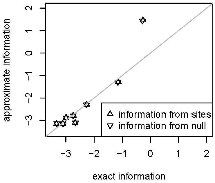
Before addressing a problem in contemporary biology, the proposed methodology will be illustrated using a simple data set that has motivated both Bayesian (Rubin, 1981) and weighted likelihood (Wang, 2006) approaches. The reduced data consist of the estimated average effect of a training program on SAT scores and an estimated standard error of the effect estimate for each of eight test sites. Following the tradition continued by Wang (2006), the standard errors $\sigma_{1},\dots,\sigma_{8}$ are considered known, and the effect estimates are modeled as normal observations with unknown means $\theta_{1},\dots,\theta_{8}$. Thus, $N=8$ and $\left\{g_{i,\theta_{i}}:\theta\in\Theta\right\}$ is the family of distributions, where $g_{i,\theta_{i}}$ is the normal density of mean $\theta_{i}$ and standard deviation $\sigma_{i}$. For the $i$th site, $\theta_{i}\neq 0$ is the alternative hypothesis and $\theta_{i}=0$ is the null hypothesis.

Fig. 1 displays $\tilde{I}_{i}\left(\mathbb{R}\backslash\left\{0\right\},\left\{0\right\}\right)$, the resulting approximate discrimination information, with $\bar{I}_{i}\left(\mathbb{R}\backslash\left\{0\right\},\left\{0\right\}\right)$, the exact discrimination information. As in Section 2.4, the weight of a single observation is assigned either to 0, the null hypothesis value (“information from null”), or to the incidental testing sites (“information from sites”). The resulting information values are barely distinguishable.

Figure 1: Information (bits) favoring the hypothesis that the test score at a site was affected by the treatment.

3.2 Single and multiple biological features

In typical experiments measuring gene expression or the abundance of proteins or metabolites, the primary question is whether the expectation value of a logarithm of the expression or abundance of each feature is affected by a treatment, disease, or other perturbation. Since that question is equivalent to that of whether $\text{CV}_{i}^{-1}$, the inverse coefficient of variation for the $i$th feature, is 0, the data reduction strategy of Example 2 often proves effective even if the magnitude of $\text{CV}_{i}^{-1}$ is not of direct interest. $\text{CV}_{i}^{-1}$ has a one-to-one correspondence to the proportion of the feature-feature pairs with abundance ratios greater than 1 (Bickel, 2004, 2008). In addition, $\text{CV}_{i}^{-1}$ is often of more scientific interest than the mean since small changes in numbers of biomolecules can have a strong influence on downstream processes.

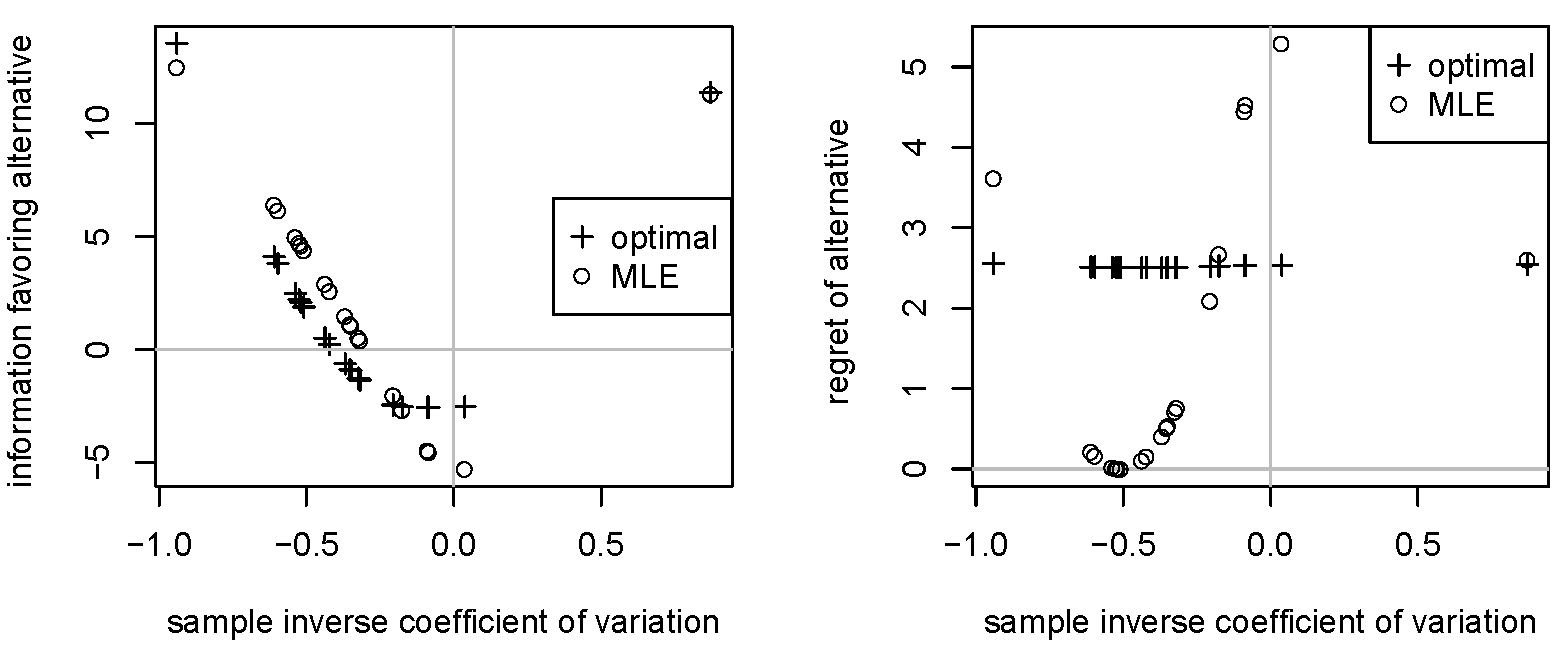
The method of Example 2 is applied to the proteomics data set of Alex Miron’s lab at the Dana-Farber Cancer Institute (Li, 2009), with $x_{ij}$ and $y_{ij}$ as the logarithms of the abundance levels of the $i$th of $N=20$ proteins in the $j$th woman with and without breast cancer, respectively, after the preprocessing of Bickel (2010b). Likewise, $\xi_{i}$ and $\eta_{i}$ are the expectation values of the random variables $X_{ij}$ and $Y_{ij}$. Each of two breast cancer groups (one of 55 HER2-positive women and the other of 35 women mostly-ER/PR-positive) were compared to a control group of 64 women. Since $\theta_{i}=\left|\text{CV}_{i}^{-1}\right|$ and thus $\Theta=\left[0,\infty\right)$, the competing hypotheses for the $i$th protein are $\theta_{i}>0$ and $\theta_{i}=0$.

The left panel of Fig. 2 displays the approximate information for discrimination in favor of the alternative hypothesis that $\theta_{i}\neq 0$ over the null hypothesis that $\theta_{i}=0$ by weighing the incidental proteins as a single observation (§2.4). $\tilde{I}_{i}\left(\left(0,\infty\right),\left\{0\right\}\right)$, the approximate optimal information, is compared to $\log\left(g_{i}\left(\hat{\theta}_{\text{MLE}};t_{i}\right)/g_{i}\left(0;t_{i}\right)\right)$. Here, $\hat{\theta}_{\text{MLE}}$ is common to all proteins, denoting the maximum likelihood estimate (MLE) defined under the assumptions that $\theta_{i}\in\left\{0,\theta_{\text{alt.}}\right\}$ for some $\theta_{\text{alt.}}>0$ for all $i$ and that the test statistics are independent (Bickel, 2010b). The right panel of Fig. 2 contrasts the widely varying regret of the MLE information with the constant regret of the optimal information.

Figure 2: Left panel: Discrimination information (bits) favoring the hypothesis that the abundance level of a protein differs by disease status versus $\widehat{\text{CV}}_{i}^{-1}$. Right panel: The corresponding regret versus $\widehat{\text{CV}}_{i}^{-1}$. ($\widehat{\text{CV}}_{i}^{-1}$ denotes the difference in sample means divided by the sample standard deviation for the $i$th protein.)

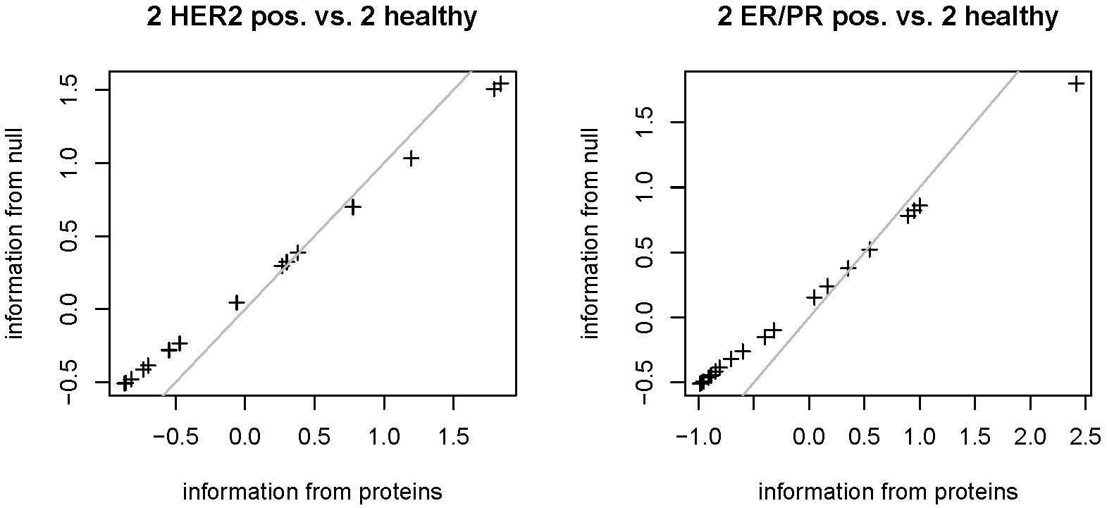
Giving the null hypothesis the weight of a single observation (11), as if the abundance level of only one protein were measured, results in information values that are visually indistinguishable from those of Fig. 2. Nonetheless, some effect of the weighting method is perceptible for much smaller sample sizes. For example, Fig. 3 displays the effect of using the null hypothesis weights instead of the protein weights on $\tilde{I}_{i}\left(\left(0,\infty\right),\left\{0\right\}\right)$ for two randomly selected patients from each breast cancer group and from the healthy group. Even in this extreme case, only one protein out of 20 in the right-side panel has a different evidence grade (Table 1) depending on how the weights are computed.

Figure 3: Discrimination information (bits) favoring the hypothesis that the abundance level of a protein differs by disease status ($n=2$ women per group) using weights from the null hypothesis versus that using weights from the incidental proteins.

4 Discussion

In both of the case studies of Section 3, the use of data associated with comparisons other than the comparison currently in focus in place of an artificial data point determined by the null hypothesis has little effect on the information for discrimination. In the second application, little information was lost for inference about a single protein were the other 19 absent except when the sample size was reduced to $n_{i}=4$. Thus, the use of single-observation weights robustly addresses the infinite-complexity issue with NML raised in Section 1.3.

The insensitivity to the use of incidental information also suggests that the NMWL solution to the incidental-information issue raised in the same section is a measure of evidence that has the same interpretation for any number of comparisons. By contrast, p-values adjusted to control error rates and, to a lesser extent, posterior probabilities from hierarchical Bayesian models, tend to vary so greatly between a single comparison and a large number of comparisons that they require researchers to separately build the intuition needed to interpret statistical reports for small numbers of comparisons, medium numbers of comparisons, large numbers of comparisons, etc. This shortcoming of traditional approaches to the multiple comparisons problem is especially glaring when an article reports various degrees of adjusting p-values for data types involving very different numbers of features.

As seen in Section 3.1, the optimal information for discrimination can indicate strong evidence for a simple null hypothesis. While in principle the Bayes factor can also favor the null hypothesis, prior distributions commonly used in practice often can provide only weak Bayes-factor support for a simple null hypothesis that corresponds to the data-generating distribution (Johnson and Rossell, 2010). The ability of the information for discrimination to indicate whether the evidence in the data is strongly in favor of the alternative hypothesis, strongly in favor of the null hypothesis, or insufficient to strongly favor either hypothesis (Table 1) guards against the prevalent misinterpretation of a high p-value as evidence for a null hypothesis. More important, the discrimination information provides scientists a reliable tool designed to objectively answer the questions they ask of their data.

References

- Berger and Pericchi (1996) Berger, J. O., Pericchi, L. R., 1996. The intrinsic Bayes factor for model selection and prediction. Journal of the American Statistical Association 91 (433), 109–122.
- Berger and Pericchi (2004) Berger, T., Pericchi, L., 2004. Training samples in objective Bayesian model selection. Annals of Statistics 32 (3), 841–869.
- Bernardo (1997) Bernardo, J. M., 1997. Noninformative priors do not exist: A discussion. Journal of Statistical Planning and Inference 65, 159–189.
- Bickel (2004) Bickel, D. R., 2004. Degrees of differential gene expression: Detecting biologically significant expression differences and estimating their magnitudes. Bioinformatics (Oxford, England) 20, 682–688.
- Bickel (2008) Bickel, D. R., 2008. Correcting the estimated level of differential expression for gene selection bias: Application to a microarray study. Statistical Applications in Genetics and Molecular Biology 7 (1), 10.
- Bickel (2009) Bickel, D. R., 2009. A frequentist framework of inductive reasoning. Technical Report, Ottawa Institute of Systems Biology, arXiv:math.ST/0602377.
- Bickel (2010a) Bickel, D. R., 2010a. Estimating the null distribution to adjust observed confidence levels for genome-scale screening. Biometrics, DOI: 10.1111/j.1541-0420.2010.01491.x.
- Bickel (2010b) Bickel, D. R., 2010b. Minimum description length methods of medium-scale simultaneous inference. Technical Report, Ottawa Institute of Systems Biology, arXiv:1009.5981.
- Bickel (2010c) Bickel, D. R., 2010c. The strength of statistical evidence for composite hypotheses: Inference to the best explanation. Technical Report, Ottawa Institute of Systems Biology, COBRA Preprint Series, Article 71, available at biostats.bepress.com/cobra/ps/art71.
- Blume and Peipert (2003) Blume, J., Peipert, J., 2003. What your statistician never told you about p-values. Journal of the American Association of Gynecologic Laparoscopists 10 (4), 439–444.
- Cornfield (1969) Cornfield, J., 1969. The Bayesian outlook and its application. Biometrics 25 (4), 617–657.
- Efron and Gous (2001) Efron, B., Gous, A., 2001. Scales of evidence for model selection: Fisher versus Jeffreys. Lecture Notes - Monograph Series 38, 208–256.
- Feifang (2002) Feifang, H.U., Z. J., 2002. The weighted likelihood. Canadian Journal of Statistics 30 (3), 347–371.
- Fisher (1973) Fisher, R. A., 1973. Statistical Methods and Scientific Inference. Hafner Press, New York.
- Fraser (2004) Fraser, D. A. S., 2004. Ancillaries and conditional inference. Statistical Science 19 (2), 333–351.
- Fraser and Reid (1990) Fraser, D. A. S., Reid, N., 1990. Discussion: An ancillarity paradox which appears in multiple linear regression. The Annals of Statistics 18 (2), 503–507.
- Gentleman et al. (2004) Gentleman, R. C., Carey, V. J., Bates, D. M., et al., 2004. Bioconductor: Open software development for computational biology and bioinformatics. Genome Biology 5, R80.
- Grünwald (2007) Grünwald, P. D., 2007. The Minimum Description Length Principle. The MIT Press, London.
- Jeffreys (1948) Jeffreys, H., 1948. Theory of Probability. Oxford University Press, London.
- Johnson and Rossell (2010) Johnson, V., Rossell, D., 2010. On the use of non-local prior densities in Bayesian hypothesis tests. Journal of the Royal Statistical Society. Series B: Statistical Methodology 72 (2), 143–170.
- Kass and Raftery (1995) Kass, R. E., Raftery, A. E., 1995. Bayes factors. Journal of the American Statistical Association 90 (430), 773–795.
- Kass and Wasserman (1995) Kass, R. E., Wasserman, L., 1995. A reference Bayesian test for nested hypotheses and its relationship to the schwarz criterion. Journal of the American Statistical Association 90 (431), 928–934.
- Kullback (1968) Kullback, S., 1968. Information Theory and Statistics. Dover, New York.
- Lanterman (2005) Lanterman, A. D., 2005. Advances in Minimum Description Length: Theory and Applications. The MIT Press, London, Ch. Hypothesis testing for Poisson versus geometric distributions using stochastic complexity, pp. 23–79.
- Li (2009) Li, X., 2009. ProData. Bioconductor.org documentation for the ProData package.
- Rissanen (1987) Rissanen, J., 1987. Stochastic complexity. Journal of the Royal Statistical Society.Series B (Methodological) 49 (3), 223–239.
- Rissanen (2007) Rissanen, J., 2007. Information and Complexity in Statistical Modeling. Springer, New York.
- Rissanen (2009) Rissanen, J., 2009. Model selection and testing by the MDL principle. Information Theory and Statistical Learning. Springer, New York, Ch. 2, pp. 25–43.
- Rissanen and Roos (2007) Rissanen, J., Roos, T., 2007. Conditional NML universal models. pp. 337–341.
- Rissanen (1996) Rissanen, J. J., 1996. Fisher information and stochastic complexity. IEEE Transactions on Information Theory 42 (1), 40–47.
- Royall (1997) Royall, R., 1997. Statistical Evidence: A Likelihood Paradigm. CRC Press, New York.
- Royall (2000) Royall, R., 2000. On the probability of observing misleading statistical evidence. Journal of the American Statistical Association 95 (451), 760–768.
- Rubin (1981) Rubin, D. B., 1981. Estimation in parallel randomized experiments. Journal of Educational Statistics 6 (4), pp. 377–401.
- Serfling (1980) Serfling, R. J., 1980. Approximation theorems of mathematical statistics. Wiley, New York.
- Severini (2000) Severini, T., 2000. Oxford University Press, Oxford.
- Shtarkov (1987) Shtarkov, Y. M., 1987. Universal sequential coding of single messages. Problems of information transmission 23 (3), 175–186.
- Sin and White (1996) Sin, C.-Y., White, H., 1996. Information criteria for selecting possibly misspecified parametric models. Journal of Econometrics 71 (1-2), 207–225.
- Sprott (2000) Sprott, D. A., 2000. Statistical Inference in Science. Springer, New York.
- Sprott (2004) Sprott, D. A., 2004. What is optimality in scientific inference? Lecture Notes-Monograph Series 44 (, The First Erich L. Lehmann Symposium-Optimality), 133–152.
- Takimoto and Warmuth (2000) Takimoto, E., Warmuth, M. K., 2000. The last-step minimax algorithm. In: ALT ’00: Proceedings of the 11th International Conference on Algorithmic Learning Theory. Springer-Verlag, London, UK, pp. 279–290.
- Wald (1961) Wald, A., 1961. Statistical Decision Functions. John Wiley and Sons, New York.
- Wang (2006) Wang, X., 2006. Approximating Bayesian inference by weighted likelihood. Canadian Journal of Statistics 34 (2), 279–298.
- Wang and Zidek (2005) Wang, X., Zidek, J. V., 2005. Derivation of mixture distributions and weighted likelihood function as minimizers of KL-divergence subject to constraints. Annals of the Institute of Statistical Mathematics 57 (4), 687–701.