Spreading Widths of Doorway States

Abstract

As a function of energy $E$, the average strength function $\overline{S(E)}$ of a doorway state is commonly assumed to be Lorentzian in shape and characterized by two parameters, the peak energy $E_{0}$ and the spreading width $\Gamma^{\downarrow}$. The simple picture is modified when the density of background states that couple to the doorway state changes significantly in an energy interval of size $\Gamma^{\downarrow}$. For that case we derive an approximate analytical expression for $\overline{S(E)}$. We test our result successfully against numerical simulations. Our result may have important implications for shell–model calculations.

1 Motivation

Giant Resonances are an ubiquitous phenomenon in nuclei [1, 2]. A specific nuclear mode with normalized wave function $|0\rangle$ carrying definite quantum numbers (spin, parity, isospin) is excited, for instance, by absorption of a gamma quantum with specific multipolarity, by nucleon–nucleus scattering, or by stripping of a nucleon from the projectile in the collision of two nuclei. The mode has a typical mean excitation energy $E_{0}$ of several or even 10 to 20 MeV, i.e., may occur above the first particle threshold. The Giant Dipole (GD) mode in nuclei is a paradigmatic case. Aside from a normalization factor, the wave function $|0\rangle$ of the GD mode is the product of the dipole operator and the eigenfunction of the nuclear ground state, and the dependence of $E_{0}$ on mass number $A$ is empirically given by $E_{0}\approx 80\ A^{-1/3}$. In general, the wave function $|0\rangle$ is not an eigenstate of the nuclear Hamiltonian $H$ and the mode is, therefore, not observed as a sharp and isolated resonance. Rather, the mode spreads in a very short time $\tau^{\downarrow}$ (typically $\tau^{\downarrow}\approx\hbar/5$ MeV $\approx 2\times 10^{-22}$ sec) over the eigenstates $|i\rangle$ of $H$ carrying the same quantum numbers (each state $|i\rangle$ corresponding to an eigenvalue $\varepsilon_{i}$ of $H$). Thus, for the particular reaction under consideration the mode $|0\rangle$ acts as a “doorway” to the eigenstates of $H$ which manifests itself as a local enhancement of the dependence on energy $E$ of the strength function

$$S(E)=\sum_{i}|\langle 0|i\rangle|^{2}\delta(E-\varepsilon_{i})\ .$$ (1)

The levels $\varepsilon_{i}$ are actually particle–unstable and, thus, resonances, and in most cases $S(E)$ is, therefore, a smooth function of $E$. Often $S(E)$ displays a broad maximum. Pending the modifications introduced below, the peak energy is then identified with the mean excitation energy $E_{0}$ of the doorway state, and the width $\Gamma^{\downarrow}$ is identified with $\hbar/\tau^{\downarrow}$ and referred to as “spreading width”. At excitation energies of $\approx 10$ MeV, the mean spacing $d$ of the nuclear levels $\varepsilon_{i}$ is typically of order $10$ eV, so that $\Gamma^{\downarrow}\gg d$. Hence the name giant resonance. Similar phenomena also occur in condensed–matter physics where the strength function $S(E)$ is commonly referred to as the local density of states.

In the simplest theoretical model [3] for the giant–resonance phenomenon, the doorway state $|0\rangle$ is coupled to a set of background states $|\mu\rangle$ (where $\mu=1,\ldots,N$ and $N\to\infty$) via real coupling matrix elements $V_{\mu}$. The background states have constant level spacing $d$. The matrix elements $V_{\mu}$ are Gaussian–distributed random variables with zero mean values and a common variance $v^{2}$. The strength function is calculated in the limit $N\to\infty$ as the average over the distribution of the $V_{\mu}$ and given by [3]

$$\overline{S(E)}=\frac{\Gamma^{\downarrow}/(2\pi)}{(E-E_{0})^{2}+(1/4)(\Gamma^{\downarrow})^{2}}\ .$$ (2)

The bar denotes the ensemble average. The average strength function has Lorentzian shape and is normalized to unity. The spreading width is given by

$$\Gamma^{\downarrow}=2\pi v^{2}/d\ .$$ (3)

Although it looks like Fermi’s golden rule, the result (3) is correct beyond perturbation theory, i.e., for all values of $v^{2}/d^{2}$.

The level density $\rho(E)$ may be taken to be constant when the rate of change with energy of $\rho(E)$ over an energy interval of length $\Gamma^{\downarrow}$ is negligible, i.e., when $[{\rm d}\ln\rho(E)/{\rm d}E]^{-1}\ll\Gamma^{\downarrow}$. In nuclei, that is not always the case. By way of example we consider the GD mode in ¹⁶O. In the shell model $|0\rangle$ is a superposition of one–particle one–hole states. Through the residual interaction $|0\rangle$ is coupled to two–particle two–hole states (two particles in the $sd$–shell and two holes in the $p$–shell). The maximum spacing in energy of the single–particle states (of the single–hole states) is about $5$ MeV [4] ($3$ MeV, respectively), giving the spectrum of the two–particle two–hole states a spectral range of about $15$ MeV. The residual interaction widens the range to $\approx 25$ MeV. The shape of the spectrum being Gaussian, the width $\sigma$ of the Gaussian is then around $15$ or $20$ MeV, and the ratio $\Gamma^{\downarrow}\approx 5$ MeV to $\sigma$ is around $1/3$ or $1/4$ and, thus, not negligible. In the present paper we show how Eq. (2) is modified under such circumstances.

Our investigation was triggered by a result for the strength function of a doorway state obtained in Ref. [5]. There we considered a Hamiltonian matrix of the form

$$H=\left(\matrix{E_{0}&V_{\nu}\cr V_{\mu}&{\cal H}_{\mu\nu}\cr}\right)\ .$$ (4)

The doorway state $|0\rangle$ at energy $E_{0}$ is coupled to $N$ background states $\mu$ with $\mu=1,\ldots,N$ and $N\to\infty$ via real matrix elements $V_{\mu}$. The background states are described by a real–symmetric random Hamiltonian matrix ${\cal H}_{\mu\nu}$, a member of the Gaussian Orthogonal Ensemble (GOE) of random matrices. The average level density of ${\cal H}_{\mu\nu}$ has the shape of a semicircle. Using the Pastur equation we calculated analytically the average strength function (the ensemble average of $S(E)$ in Eq. (1)). Whenever the value of the spreading width $\Gamma^{\downarrow}$ given by Eq. (3) was not negligible in comparison to the radius $2\lambda$ of the GOE semicircle, the effective spreading width $\Gamma_{\rm eff}$ (defined as the full width at half maximum of the average strength function) turned out to be bigger than $\Gamma^{\downarrow}$, the increase being proportional to $\Gamma^{\downarrow}/\lambda$. The method of derivation in Ref. [5] was confined to the GOE with its unrealistic semicircular spectral shape. In the present paper we present an approach that, although more approximate than that of Ref. [5], applies for a coupling of the doorway state to background states with a general dependence of the average level density $\rho(E)$ on energy $E$. We determine how the effective spreading width $\Gamma_{\rm eff}$ differs from $\Gamma^{\downarrow}$ as given by Eq. (3) when $\rho(E)$ is not constant.

The model of Ref. [3] disregards all details of nuclear structure. In a more realistic approach, one has to replace the statistical assumptions on the matrix elements $V_{\mu}$ and the assumption of a constant level spacing $d$ by a nuclear–structure model like the shell model and/or one of the collective models. In these approaches, the damping mechanism has received considerable attention [6, 1, 2], with special focus on the GD resonance [7]. Because of the large number of states that couple to the doorway state, the effort is substantial, however, and the simple statistical model of Ref. [3], i.e., the use of Eq. (2) together with a calculation of $\Gamma^{\downarrow}$ from Eq. (3), continues to play an important role in the analysis of giant–resonance phenomena in nuclei. For that reason we revisit and extend the model in the present paper.

2 Model

Similarly to Eq. (4) we model the doorway state by the Hamiltonian matrix

$$H=\left(\matrix{E_{0}&V_{\nu}\cr V_{\mu}&E_{\mu}\delta_{\mu\nu}\cr}\right)$$ (5)

where the index $\mu$ ranges from $1$ to $N$ with $N\gg 1$. The matrix (5) differs formally from that of Eq. (4) in that ${\cal H}_{\mu\nu}$ has been diagonalized. Instead of the statistical assumptions on the matrix ${\cal H}_{\mu\nu}$ made below Eq. (4), we assume that the $V_{\mu}$ are Gaussian random variables with zero mean value and a second moment $v^{2}$, and that they are not correlated with the $E_{\mu}$. We do not need any assumptions on the distribution of the latter. Thus, our model is more general than the random–matrix model of Ref. [5].

To calculate the strength function $S(E)$, we rewrite Eq. (1) as

$$S(E)=-\frac{1}{\pi}\ \Im\bigg{(}\langle 0|\frac{1}{E^{+}-H}|0\rangle\bigg{)}$$ (6)

where $E^{+}=E+i\epsilon$ with $\epsilon$ positive infinitesimal. Using Eq. (5) we obtain [6, 3]

$$S(E)=-\frac{1}{\pi}\ \Im\bigg{(}\frac{1}{E^{+}-E_{0}-\sum_{\mu}V_{\mu}(E^{+}-E_{\mu})^{-1}V_{\mu}}\bigg{)}\ .$$ (7)

Prior to calculating the ensemble average of $S(E)$ we calculate the ensemble average of the sum over $\mu$ in the denominator of Eq. (7). That sum is denoted by $\Sigma$. The average over the distribution of the $V_{\mu}$ gives

$$\overline{\Sigma}^{V}=v^{2}\sum_{\mu}(E^{+}-E_{\mu})^{-1}\ .$$ (8)

For the remaining sum over $\mu$ we write

$$F(E)=\sum_{\mu}\frac{1}{E^{+}-E_{\mu}}=\int{\rm d}E^{\prime}\ \frac{1}{E^{+}-E^{\prime}}\sum_{\mu}\delta(E^{\prime}-E_{\mu})\ .$$ (9)

Averaging over the distribution of the $E_{\mu}$, we replace $\sum_{\mu}\delta(E^{\prime}-E_{\mu})$ by $\rho(E)$, the average level density of the background states, and obtain

$$\overline{F(E)} = \int{\rm d}E^{\prime}\ \frac{1}{E^{+}-E^{\prime}}\rho(E^{\prime})$$ (10)

$$= -i\pi\rho(E)+\int{\rm d}E^{\prime}\ \frac{\cal P}{E-E^{\prime}}\rho(E^{\prime})$$

where ${\cal P}$ indicates the principal–value integral. Thus,

$$\overline{\Sigma}=-i\pi v^{2}\rho(E)+v^{2}\int{\rm d}E^{\prime}\ \frac{\cal P}{E-E^{\prime}}\rho(E^{\prime})\ .$$ (11)

We show presently that for $N\to\infty$ and $\Gamma^{\downarrow}\gg d$ the average strength function $\overline{S(E)}$ is obtained by replacing in Eq. (7) the function $\Sigma(E)$ by $\overline{\Sigma}$. That yields

$$\overline{S(E)}=\frac{1}{2\pi}\ \frac{\Gamma^{\downarrow}}{(E-E_{0}-\Delta)^{2}+(1/4)(\Gamma^{\downarrow})^{2}}$$ (12)

where

$$\Gamma^{\downarrow} = 2\pi v^{2}\rho(E)\ ,$$

$$\Delta = v^{2}\int{\rm d}E^{\prime}\ \frac{\cal P}{E-E^{\prime}}\ \rho(E^{\prime})\ .$$ (13)

Eqs. (12) and (13) obviously generalize Eqs. (2) and (3) to the case where $\rho(E)$ is not constant and reduce to the latter if it is.

To justify our averaging procedure (replacement of $\Sigma$ by $\overline{\Sigma}$) we consider first the average of $S(E)$ over the Gaussian–distributed matrix elements $V_{\mu}$. We use the property that the average of the product $V_{\mu}V_{\nu}V_{\rho}V_{\sigma}$ has the value $(v^{2})^{2}[\delta_{\mu\nu}\delta_{\rho\sigma}+\delta_{\mu\rho}\delta_{\nu\sigma}+\delta_{\mu\sigma}\delta_{\nu\rho}]$, and similarly for higher–order terms. In other words, averages over products of Gaussian random variables are calculated by Wick contraction of all pairs. For each pair the average is zero unless the indices are equal. The average of $S(E)$ in Eq. (7) can be calculated by expanding the denominator in powers of the $V$s and using Wick contraction. After averaging, the leading contribution to each term of the series is the one where $V$s appearing pairwise under the same summation over $\mu$ are averaged. All other Wick contractions restrict the independent summations over $\mu$ and lead to terms that are small of order $1/N$ and, thus, negligible for $N\gg 1$. Hence to leading order in $1/N$ averaging $S(E)$ in Eq. (7) over the $V_{\mu}$ is equivalent to averaging $\Sigma$.

We turn to the average over the $E_{\mu}$ and use that $S(E)$ depends on the $E_{\mu}$ only via the expression $\sum_{\mu}\delta(E-E_{\mu})$. Expanding $S(E)$ in powers of $\Sigma$ and averaging over the $E_{\mu}$ we see that our averaging procedure is justified if the $E_{\mu}$ are uncorrelated. Then, in each term of the series $\sum_{\mu}\delta(E-E_{\mu})$ is replaced by $\rho(E)$ and the result is the same as replacing $\Sigma$ in $S(E)$ by $\overline{\Sigma}$. The strongest known correlations among eigenvalues are those of the GOE where the $E_{\mu}$ follow Wigner–Dyson statistics. GOE level correlations extend over an energy range measured in units of $d$ while $\overline{S(E)}$ varies with energy over an interval of length $\Gamma^{\downarrow}$. Therefore, such correlations produce correction terms in the expansion of $S(E)$ in powers of $\Sigma$ that are small of order $d/\Gamma^{\downarrow}$ and are, thus, negligible for $\Gamma^{\downarrow}\gg d$. The argument does not apply near the end points of the spectrum where the level density tends to zero and $d$ becomes large. This suggests that for our approximation to be valid the distance of $E_{0}$ from the end points of the spectrum should be larger than $\Gamma^{\downarrow}$. We observe, however, that equations (12) and (13) provide reasonable approximations to our numerical results even when that condition fails.

We conclude that Eqs. (12) and (13) for the average strength function $\overline{S(E)}$ of a doorway state are valid except perhaps near the end points of the spectrum. These equations generalize Eqs. (2) and (3) by the appearance of a shift function $\Delta(E)$. As shown by the second of Eqs. (13) that function accounts for level repulsion between the doorway state and the background states. The function $\Delta(E)$ receives negative (positive) contributions from background states that lie above (below) the energy $E$. If the spectrum is symmetric about $E=0$ then $\Delta(0)=0$ and $\Delta(E)<0$ ($\Delta(E)>0$) if $E<0$ ($E>0$, respectively). For a doorway state at $E_{0}=0$ this fact widens the spectrum and causes $\Gamma_{\rm eff}$ to be larger than $\Gamma^{\downarrow}$ as given by the first of Eqs. (13). Obviously, our result agrees with Eqs. (2) and (3) if the average level density of the background states is constant so that $\Delta=0$. The shift function $\Delta(E)$ is very similar to the shift function for a scattering resonance due to its interaction with a continuum of scattering states [8, 9, 10].

We display the dimensionless ratio $\Delta(E)/\Gamma^{\downarrow}(0)$ for two important examples: The average level density has the shape of a semicircle (the case of the GOE) or of a Gaussian (this is typical of level densities in the shell–model [4]). With the normalization $\int{\rm d}E\ \rho(E)=N$ we have

$$\rho(E) = \frac{N}{\pi\lambda}\sqrt{1-\bigg{(}\frac{E}{2\lambda}\bigg{)}^{2}}\ \ {\rm(semicircle)}\ ,$$

$$\rho(E) = \frac{N}{\sqrt{2\pi}\lambda}\exp[-E^{2}/(2\lambda^{2})]\ \ {\rm(Gaussian)}\ .$$ (14)

Here $\lambda$ denotes half the radius of the semicircle (the variance of the Gaussian, respectively). With $x=E/\lambda$ the ratio $\Delta(E)/\Gamma^{\downarrow}(0)$ is given by

$$\Delta(E)/\Gamma^{\downarrow}(0) = \frac{1}{2\pi}\int_{-2}^{+2}{\rm d}x^{\prime}\ \frac{\cal P}{x-x^{\prime}}\sqrt{1-x^{\prime 2}/4}$$

$$= \frac{x}{4}-[\theta(2+x)-\theta(2-x)]\frac{1}{2}\sqrt{\frac{x^{2}}{4}-1},\ \ {\rm(semicircle)},$$

$$\Delta(E)/\Gamma^{\downarrow}(0) = \frac{1}{2\pi}\int_{-\infty}^{+\infty}{\rm d}x^{\prime}\ \frac{\cal P}{x-x^{\prime}}\exp[-x^{\prime 2}/2]$$ (15)

$$= \frac{1}{2}{\rm e}^{-x^{2}/2}(-i){\rm erf}(i\frac{x}{\sqrt{2}})\ \ {\rm(Gaussian)}.$$

Fig. 1 displays these two functions versus $x$. W conclude that $\Delta(E)$ is significant whenever $\Gamma^{\downarrow}/\lambda$ is not negligibly small.

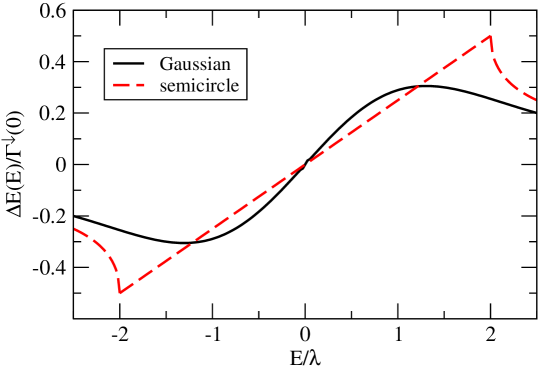
Figure 1: Plot of the functions $\Delta(E)/\Gamma^{\downarrow}(0)$ in Eqs. (15) versus $E/\lambda$ for the semicircle (dashed, color online: red) and the Gaussian (solid, color online: black).

To estimate the effect of the values of $\Delta(E)$ displayed in Fig. 1 on the strength function, we note that for the semicircle, the function $\Delta(E)$ is linear in $E$ over the entire range of the spectrum while in the Gaussian case, $\Delta(E)$ is approximately linear near the center of the spectrum. For both cases we write

$$\Delta(E)\approx\alpha x\Gamma^{\downarrow}(0)=\alpha E\ (\Gamma^{\downarrow}(0)/\lambda)=\alpha E\gamma$$ (16)

where $\gamma=\Gamma^{\downarrow}(0)/\lambda$ and where $\alpha>0$ is dimensionless. Substituting that expression into Eq. (12) we obtain

$$\overline{S(E)}=\frac{1}{2\pi}\ \frac{1}{1-\alpha\gamma}\ \frac{\Gamma_{\rm eff}}{(E-\tilde{E}_{0})^{2}+\Gamma_{\rm eff}^{2}/4}$$ (17)

where

$$\tilde{E}_{0}=E_{0}/(1-\alpha\gamma)\ {\rm and}\ \Gamma_{\rm eff}=\Gamma^{\downarrow}/(1-\alpha\gamma)\ .$$ (18)

The factor $1/(1-\alpha\gamma)>1$ shifts the mean energy $E_{0}$ of the doorway state towards smaller (larger) values when $E_{0}<0$ ($E_{0}>0$, respectively) and increases the effective value of the spreading width. The value of $\alpha$ is obtained by differentiating $\Delta(E)$ at $E=0$. For the semicircle we find $\alpha=1/4$, in agreement with the result of Ref. [5]. For the Gaussian we have $\alpha=1/\sqrt{2\pi}$. In both cases and with $\gamma\approx 1/3$ or $1/4$, that gives a correction of about $10$ to $20$ percent to both $E_{0}$ and $\Gamma^{\downarrow}$.

In summary, Eqs. (12) and (13) are expected to provide a better approximation to $\overline{S(E)}$ than Eqs. (2) and (3) if $\rho(E)$ changes significantly over an energy interval of length $\Gamma^{\downarrow}$. Then we expect the full width $\Gamma_{\rm eff}$ at half maximum of $\overline{S(E)}$ to be bigger than $\Gamma^{\downarrow}$ as given by the first of Eqs. (13). Eqs. (12) and (13) may fail near the end points of the spectrum of the background states. This is in accord with the exact results of Ref. [5]. There it was shown that the interaction with the doorway state increases the range the GOE spectrum. Such an effect is beyond the scope of the present approximate treatment.

3 Numerical Simulation

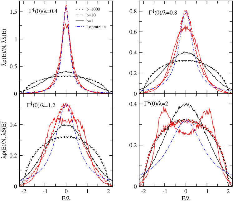
Figure 2: Strength functions (color online: red) of a doorway state at $E_{0}=0$ coupled to background states described by a random band matrix of dimension $N=1000$ and bandwidth $b$ as defined in the text; the coupling matrix elements are uncorrelated Gaussian-distributed random variables (case (i) of the text). For comparison, we also display the Lorentzian distribution of Eqs. (2) and (3) (color online: blue). The average level densities of the background states are also shown (color online: black). Each panel corresponds to a fixed value $\Gamma^{\downarrow}(0)/\lambda$ of the spreading width of Eq. (3). Averages are performed over $m=500$ realizations.

Figure 3: Same as for Fig. 2 but only for $b=1$ (diagonal random band matrix) and for $b=1000$ (GOE matrix). In addition to the curves shown previously we now display also the predictions of Eqs. (12) and (13) (color online: blue).

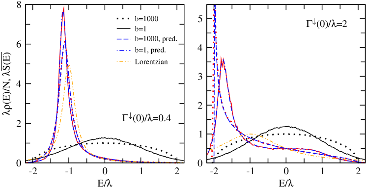
Figure 4: Same as for Fig. 2 at $E_{0}/\lambda=-1$, but only for $b=1$ (diagonal random band matrix) and for $b=1000$ (GOE matrix). We also display the predictions of Eqs. (12) and (13) (color online: blue) and of Eqs. (2) and (3) (color online: orange).

Figure 5: Full width at half maximum $\Gamma_{\rm eff}$ of the average strength function of the doorway state, displayed as a function of the input width $\Gamma^{\downarrow}(0)$ of Eq. (3). The circles represent results of the numerical diagonalization, the lines correspond to Eqs. (12) and (13).

To test the approximations leading to Eqs. (12) and (13) we consider a doorway state coupled to a random band matrix. Random band matrices have been frequently used in different physical contexts. The model is that of Eq. (4) except that ${\cal H}_{\mu\nu}$ is a real symmetric random band matrix of dimension $N$: All matrix elements with $|\mu-\nu|\geq b$ vanish. The upper bound on the number of non–zero elements in every row and column is $(2b-1)$. The non–vanishing matrix elements are uncorrelated Gaussian–distributed random variables with variances given by $\overline{{\cal H}^{2}_{\mu\nu}}=(1+\delta_{\mu\nu})\beta^{2}$. For $b=1$ the matrix ${\cal H}_{\mu\nu}$ is diagonal while for $b=N$ it is equal to the GOE. To make sure that all spectra have approximately the same width we determine $\beta^{2}$ from the condition $(1/N){\rm Trace}\overline{{\cal H}^{2}}=\lambda^{2}$. That gives

$$\beta^{2}=\frac{\lambda^{2}}{2b-\frac{\displaystyle b(b-1)}{\displaystyle N}}.$$ (19)

The average spectrum of the random band matrix ${\cal H}_{\mu\nu}$ is Gaussian for $b=1$ and changes quickly into an approximately semicircular form as $b$ is increased [11]. For $N=1000$, we found that the average spectrum is much more similar to a semicircle than to a Gaussian already for $b=5$; the transition to semicircular shape was virtually complete at $b=100$. For $b<\sqrt{N}$ and $N\gg 1$ the eigenfunctions of a random band matrix are localized, and the eigenvalues are uncorrelated, i.e., have Poissonian statistics [11]. Indeed, for $N=1000$ the nearest–neighbor spacing distribution changes from Poisson to Wigner form near $b=30$. Similarly, the inverse participation ratio defined below decreases strongly with increasing $b$. Some of these results are displayed in the figures shown below. As a consequence, random band matrices are useful for testing our approximations both for a Gaussian spectrum ($b=1$) and for a spectrum with Poisson statistics ($b<\sqrt{N}$).

We have considered two ways of coupling the doorway state with the random band matrix ${\cal H}_{\mu\nu}$: (i) The coupling matrix elements $V_{\mu}$ in Eq. (4) are uncorrelated Gaussian–distributed random variables with zero mean values and a common second moment $v^{2}$. Then the doorway state is coupled to all states in ${\cal H}_{\mu\nu}$ irrespective of the value of $b$, i.e., irrespective of the localization properties of the eigenvectors of ${\cal H}_{\mu\nu}$. (ii) We take $V_{\mu}=0$ for all $\mu=1,\ldots,N$ except for $\mu$–values in a band of width $w$ centered in the interval $[1,N]$. The doorway state is coupled only to select states in ${\cal H}_{\mu\nu}$. Localization properties of the random band matrix should influence the value of the average strength function of the doorway state. In case (ii) the non–vanishing matrix elements were taken to have all the same value $v\sqrt{N/w}$. Then the total coupling strength $\sum_{\mu}V^{2}_{\mu}$ is on average the same in cases (i) and (ii).

The input parameters of the model are $b,w,v^{2},E_{0}$, and $N$ while $\lambda$ defines the spectral width and, thus, the energy scale. A further input parameter is $m$, the number of independent drawings of the matrix elements ${\cal H}_{\mu\nu}$ from a random–number generator. Each such drawing produces a realization of the random matrix (4). Diagonalization of that matrix yields the eigenvalues $\varepsilon_{i}$ and eigenfunctions $|i\rangle$. These are used to generate the strength function in Eq. (1). Combining $m$ realizations we obtain the average strength function $\overline{S(E)}$. That function is compared with Eqs. (12) and (13).

For case (ii) with parameter $w=1$ the doorway state with energy $E_{0}$ is coupled to only a single other state with Gaussian–distributed energy $\varepsilon$, and the average strength function $\overline{S(E)}$ can be calculated analytically. We find

$$\overline{S(E)}=\frac{1}{\sqrt{\pi}\lambda}\frac{v^{2}}{(E_{0}-E)^{2}}\left.{\rm e}^{-\epsilon^{2}/\lambda^{2}}\right|_{\epsilon=E+\frac{v^{2}}{(E_{0}-E)}}\ .$$ (20)

The function $\overline{S(E)}$ vanishes at $E=E_{0}$, extends over the entire spectrum, and has two maxima on opposite sides of $E=E_{0}$. That is a consequence of level repulsion and explains qualitatively some of the features seen in the figures shown below.

In Figs. 2 to 5 we present numerical results for case (i). In Fig. 2 we display strength functions for parameter values indicated in the figure. The discrepancy between the predictions of Eqs. (2) and (3) and the actual values of the strength function are obvious and increase with increasing values of the spreading width $\Gamma^{\downarrow}$. We note the gradual development of a dip at $E_{0}=0$ and of a double–hump of the strength function. We believe that these features correspond to properties of the simple model of Eq. (20). In Fig. 3 we compare some of these results with the predictions of Eqs. (12) and (13) and find very good agreement. We note that the dip is correctly reproduced. We have performed similar calculations for non–zero values of $E_{0}$ and found that the Lorentzian model shows even larger discrepancies, since it is not able to reproduce not only the correct width, but also the asymmetric shape that develops for $E_{0}\neq 0$. On the other hand, Eqs. (12) and (13) provide the same good agreement for every value of $E_{0}$. An example is shown in Fig. 4 for the case of $E_{0}/\lambda=-1$, while our results are summarized in Fig. 5. We believe that the agreement of the numerical results with Eqs. (12) and (13) is impressive. We also note that $\Gamma_{\rm eff}$ and $\Gamma^{\downarrow}$ differ significantly.

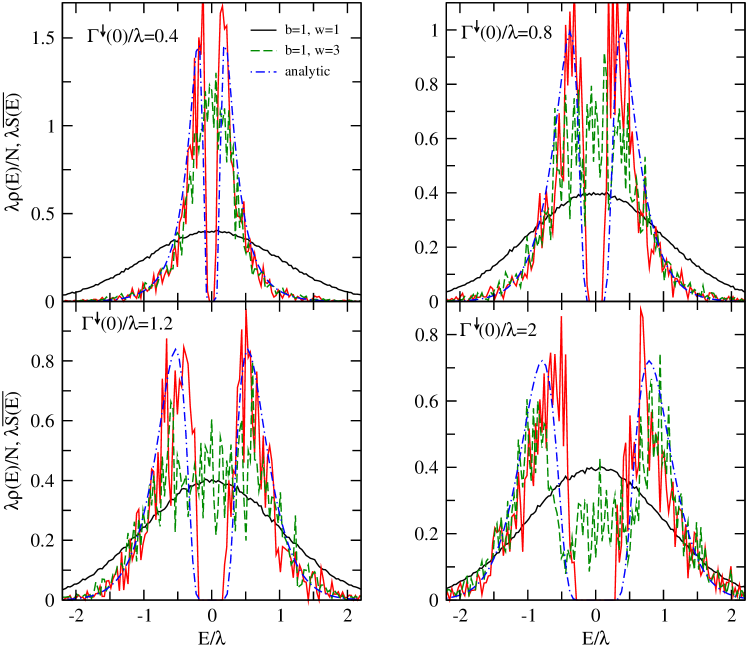
Figure 6: The average strength function (color online: red) for a doorway state coupled to a random band matrix with $b=1$ of dimension $N=1000$ (case (ii) of the text) is compared with the analytical result of Eq. (20) (color online: blue). The average level density of the backgound states is also shown (color online: black). The value of $\Gamma^{\downarrow}(0)/\lambda$ is given in each panel. The dashed lines (color online: green) show the strength function when the number of states directly coupled to the doorway state is increased from one to three.

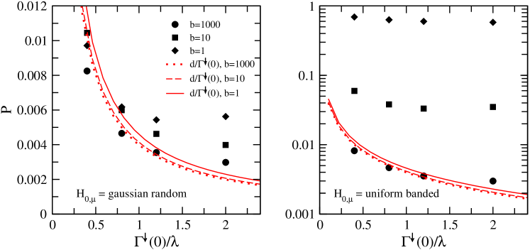
Figure 7: Inverse participation ratio of the doorway state as a function of the input spreading width $\Gamma^{\downarrow}/\lambda$ for $N=1000$ and several values of $b$ as shown in the panels. In the left panel the coupling matrix elements are uncorrelated Gaussian–distributed random variables (case (i) of the text), while in the right panel they are equal and restricted to a band of width $w=b$ (case (ii) of the text). The average level spacing of each matrix ensemble is denoted by $d$.

We turn to case (ii). Again we have performed calculations for $N=1000$. Case (ii) agrees with case (i) for $b=1000$. The results for $b=10$ are qualitatively similar to those of case (i). Therefore, we focus attention on the case $b=1$ and consider $E_{0}=0$. Results are shown and compared with the exact analytical result of Eq. (20) in Fig. 6. The double hump is clearly displayed. The agreement is very good as expected. Similarly good agreement was found when $E_{0}$ was chosen different from zero. On the other hand, a comparison of Fig. 6 and the results of Eqs. (12) and (13) displayed in Fig. 3 shows that the approximations leading to Eqs. (12) and (13) fail when the doorway state is coupled to a single background state only (the case $w=1$ in Fig 6). That is a very special situation and not typical for doorway states. Increasing the number of background states to which the doorway is coupled but keeping the bandwidth of ${\cal H}_{\mu\nu}$ unchanged, very quickly changes the strength function so that approximate agreement with Eqs. (12) and (13) is attained. For $w=3$ that is shown by the dashed lines (color online: green) in Fig. 6.

To understand the role of localization in the mixing of the doorway state with the background states we have calculated the average inverse participation ratio (IPR) of the doorway state. The IPR is defined in terms of the amplitudes $\langle 0|i\rangle$ of the expansion of the doorway state in the basis of eigenfunctions $|i\rangle$, $i=0,1,\ldots,N$ of the matrix (4) as $\sum_{i}\overline{|\langle 0|i\rangle|^{4}}$. If the doorway state is spread more or less uniformly over the eigenstates then the normalization condition $\sum_{i}|\langle 0|i\rangle|^{2}=1$ suggests that the IPR has a value around $1/N$. If, on the other hand, the doorway state mixes with only a few of the eigenstates then the IPR should be much larger than $1/N$. Thus, for case (i) we expect values of the IPR around $1/N$ and for case (ii) much bigger values. The left panel of Fig. 7 corresponds to case (i). The IPR (black dots) decreases as $\Gamma^{\downarrow}$ increases. The values for $b=1$ are somewhat larger than those for $b=1000$ but still close to $1/N$. The solid, dashed and dashed–dotted lines are obtained from the simple estimate $d/\Gamma^{\downarrow}(0)$ for the IPR. For case (ii) (right panel) and $b=1$ and $b=10$ the IPR is significantly larger than $1/N$ and roughly given by $1/b$. That shows that the doorway state mixes only with few ($\approx b$) states.

4 Conclusions

We have investigated the strength function of a doorway state coupled to a number of background states in cases of strong coupling (the spreading width $\Gamma^{\downarrow}$ is not small compared to the range of the spectrum of background states). Our result in Eqs. (12) and (13) generalizes the standard weak–coupling result and agrees with it for weak coupling. We have tested our result by numerical simulations. In most cases studied, we found perfect agreement between the numerical results and Eqs. (12) and (13). Exceptions are found only when the doorway is coupled to a single background state. That situation is atypical. Even when the number of directly coupled states is increased from one to three, approximate agreement with Eqs. (12) and (13) is attained.

We have pointed out that the strong–coupling case is of practical interest and may actually play a role in shell–model calculations. That is the case whenever the spreading width $\Gamma^{\downarrow}$ is not very small compared to the range in energy over which the average level density of the background states changes significantly. Then our Eqs. (12) and (13) offer a more accurate description of the strength function of the doorway state than do the standard Eqs. (2) and (3). Typically the full width at half maximum $\Gamma_{\rm eff}$ of the average strength function is then larger than the theoretical expression $\Gamma^{\downarrow}=2\pi v^{2}\rho(E)$. The difference may be important for a comparison between theory and data.

When the doorway state couples to a random band matrix with localized eigenfunctions and when the coupling involves only a narrow band of states (our case (ii)), we have found that the inverse participation ratio of the doorway state is considerably larger than the inverse matrix dimension. That shows that the doorway state mixes only with a restricted number of localized states. The result is important for practical applications. Indeed, in the nuclear shell model the doorway state (a 1p 1h state) mixes with 2p 2h states which have a Gaussian spectrum. But because of the presence of other modes of excitation, the actual nuclear spectrum is not Gaussian in shape but increases monotonically with energy, and one may ask what significance our results have in view of this fact. However, the mixing of the 2p 2h states with such other states is weak (otherwise shell structure would not persist). Modeling such weak mixing in terms of a random band matrix with localization, we have shown that our results remain valid in the presence of other modes of excitation.

References

- [1] P. F. Bortignon, A. Bracco, and R. A. Broglia, Giant Resonances. Nuclear Structure at Finite Temperature, Harwood Academic, New York, 1998.
- [2] M. N. Harakeh, A. van der Woude, Giant Resonances: Fundamental High–Energy Modes of Nuclear Excitation, Oxford University Press, Oxford, 2001.
- [3] A. Bohr and B. R. Mottelson, Nuclear Structure, Volume 1, W. A. Benjamin, New York, 1968.
- [4] V. Zelevinsky, B. A. Brown, N. Frazier, and M. Horoi, Phys. Rep. 276 (1996) 85.
- [5] A. De Pace, A. Molinari, and H. A. Weidenmüller, Ann . Phys. (N.Y.) 322 (2007) 2446.
- [6] G. F. Bertsch, P. F. Bortignon, and R. A. Broglia, Rev. Mod. Phys. 55 (1983) 287.
- [7] D. Sarchi, P. F. Bortignon, and G. Colo, Phys. Lett. B 601 (2004) 27.
- [8] J. B. Ehrman, Phys. Rev. 81 (1951) 412.
- [9] R. G. Thomas, Phys. Rev. 88 (1952) 1109.
- [10] G. E. Mitchell, A. Richter, and H. A. Weidenmüller, Rev. Mod. Phys. (in press) and arXiv 1001.2422.
- [11] G. Casati, L. Molinari, and F. Izrailev, Phys. Rev. Lett. 64 (1990) 1851.