Generalised shape theory via pseudo-Wishart distribution

Abstract

The non isotropic noncentral elliptical shape distributions via pseudo-Wishart distribution are founded. This way, the classical shape theory is extended to non isotropic case and the normality assumption is replaced by assuming a elliptical distribution. In several cases, the new shape distributions are easily computable and then the inference procedure can be studied under exact densities. An application in Biology is studied under the classical gaussian approach and two non gaussian models.

1 Introduction

With the introduction of several innovative statistical and mathematical tools for high-dimensional data analysis, now the classical multivariate analysis have a new and modern image. Developments as generalised multivariate analysis, latent variable analysis, DNA microarray data, pattern recognition, multivariate analysis nonlinear, data mining, manifold learning, shape theory, etc., open a range of potential applications in many areas of the knowledge.

As consequence of these new statistical and mathematical tools a new theory can be considere from the conjunction between generalised multivariate analysis and the statistical shape theory is termed Generalised Shape Theory, in which the methodology developed in the shape theory under Gaussian models is extended to a general class of distributions, the elliptically contoured densities.

Having this goal in mind, recall that $\mathbf{X}:N\times K$ has a matrix multivariate elliptically contoured distribution if its density with respect to the Lebesgue measure on $\Re^{NK}$ is given by:

$$f_{\mathbf{X}}(\mathbf{X})=\frac{1}{|\mathbf{\Sigma}|^{K/2}|\mathbf{\Theta}|^{N/2}}h\left\{\mathop{\rm tr}\nolimits\left[(\mathbf{X}-\boldsymbol{\mu})^{\prime}\mathbf{\Sigma}^{-1}(\mathbf{X}-\boldsymbol{\mu})\mathbf{\Theta}^{-1}\right]\right\},$$

where $\boldsymbol{\mu}:N\times K$, $\mathbf{\Sigma}:N\times N$, $\mathbf{\Theta}:K\times K$, $\mathbf{\Sigma}$ positive definite ($\mathbf{\Sigma}>\mathbf{0}$), $\mathbf{\Theta}>\mathbf{0}$. The function $h:\Re\rightarrow[0,\infty)$ is termed the generator function, and it is such that $\int_{0}^{\infty}u^{NK-1}h(u^{2})du<\infty$. Such a distribution is denoted by $\mathbf{X}\sim\mathcal{E}_{N\times K}(\boldsymbol{\mu},\mathbf{\Sigma},\mathbf{\Theta},h)$, see Fang and Zhang (1990) and Gupta and Varga (1993). Observe that this class of matrix multivariate distributions includes Gaussian, Contaminated Normal, Pearson type II and VI, Kotz, Jensen-Logistic, Power Exponential, Bessel, among other distributions; whose distributions have tails that are weighted more or less, and/or distributions with greater or smaller degree of kurtosis than the Gaussian model.

Now, in shape theory context, it is known that the shape of an object is all geometrical information that remains after filtering out translation, rotation and scale information of an original figure (represented by a matrix $\mathbf{X}$) comprised in $N$ landmarks in $K$ dimensions. Hence, we say that two figures, $\mathbf{X}_{1}:N\times K$ and $\mathbf{X}_{2}:N\times K$ have the same shape if they are related with a special similarity transformation $\mathbf{X}_{2}=\beta\mathbf{X}_{1}\mathbf{H}+\mathbf{1}_{N}\boldsymbol{\gamma}^{\prime}$, where $\mathbf{H}:K\times K\in SO(K)=\{\mathbf{H}\in\Re^{K\times K}|\mathbf{HH}^{\prime}=\mathbf{H}^{\prime}\mathbf{H}=\mathbf{I}_{K}\mbox{ and }|\mathbf{H}|=+1\}$ (the rotation), $\boldsymbol{\gamma}:K\times 1$ (the translation), $\mathbf{1}_{N}:N\times 1,$ $\mathbf{1}_{N}=(1,1,\ldots,1)^{\prime}$, and $\beta>0$ (the scale). Thus, in this context, the shape of a matrix $\mathbf{X}$ is all the geometrical information about $\mathbf{X}$ that is invariant under Euclidean similarity transformations, see Goodall and Mardia (1993) and Dryden and Mardia (1998).

In the classical statistical shape theory is assumed that $\mathbf{X}$ has the isotropic matrix multivariate Gaussian distribution with mean $\boldsymbol{\mu}_{\mathbf{X}}$, see Goodall and Mardia (1993), i.e.

$$\mathbf{X}\sim\mathcal{N}_{N\times K}(\boldsymbol{\mu}_{\mathbf{X}},\sigma^{2}\mathbf{I}_{N}\otimes\mathbf{I}_{K}).$$

In the context of the generalised shape theory, it is assumed that

$$\mathbf{X}\sim\mathcal{E}_{N\times K}(\boldsymbol{\mu}_{{}_{\mathbf{X}}},\mathbf{\Sigma}_{{}_{\mathbf{X}}}\otimes\mathbf{\Theta},h).$$

Thus, two fundamental extensions of classical shape theory are provided, namely:

• The generalised theory assumes a matrix multivariate elliptical distribution for the landmark data instead of considering a matrix multivariate Gaussian distribution.

• Also, the usual isotropic Gaussian condition is replaced by assuming a non isotropic elliptical model. Two important advantages are obtained: first, the errors are correlated among landmarks, this is considered with the introduction of $\mathbf{\Sigma}$, a $N\times N$ definite positive matrix; and second, the errors are correlated among coordinates of landmarks, this condition is noticed with the introduction of $\mathbf{\Theta}$, a $K\times K$ definite positive matrix.

The shape coordinates denoted as $\mathbf{u}$ of $\mathbf{X}$ can be constructed by several ways in terms of QR decomposition, see Goodall and Mardia (1993); and singular value decomposition (SVD), see Goodall (1991), Le and Kendall (1993) and Goodall and Mardia (1993). For example, in terms of the QR decomposition, shape coordinates $\mathbf{u}$ of $\mathbf{X}$ are constructed in several steps summarised in the expression

$$\mathbf{L}\mathbf{X}\mathbf{\Theta}^{-1/2}=\mathbf{L}\mathbf{Z}=\mathbf{Y}=\mathbf{TH}=r\mathbf{WH}=r\mathbf{W}(\mathbf{u})\mathbf{H},$$ (1)

Observe that $\boldsymbol{\mu}_{{}_{\mathbf{Z}}}=\boldsymbol{\mu}_{{}_{\mathbf{X}}}\mathbf{\Theta}^{-1/2}$ and the QR shape coordinates of $\boldsymbol{\mu}_{{}_{\mathbf{Z}}}$ are defined analogously. The matrix $\mathbf{L}:(N-1)\times N$ has orthonormal rows to $\textbf{1}=(1,\ldots,1)^{\prime}$. $\mathbf{L}$ can be a submatrix of the Helmert matrix, for example. Now, let be $n=\min(N-1,K)$ and $p=\mathop{\rm rank}\nolimits\mu$. In (1), $\mathbf{Y}=\mathbf{TH}$ is the QR decomposition, where $\mathbf{T}:(N-1)\times n$ is lower triangular with $t_{ii}>0$, $i=1,\ldots,\min(n,K-1)$, and $\mathbf{H}:n\times K$, $\mathbf{H}\in\mathcal{V}_{n,K}=\{\mathbf{H}\in\Re^{n\times K}|\mathbf{HH}^{\prime}=\mathbf{I}_{n}\}$, the Stiefel manifold. Note that $\mathbf{T}$ is invariant to translations and rotations of $\mathbf{Z}$. The matrix $\mathbf{T}$ is referred as the QR size-and-shape and their elements are the QR size-and-shape coordinates of the original landmark data $\mathbf{Z}$. Typically in shape analysis there are more landmarks than dimensions ($N>K$). $\mathbf{H}$ acts on the right to transform $\Re^{K}$ instead of acting on the left as in the multivariate analysis. In our case we see the landmarks as variables and the dimensions as observations, then the transposes of our matrices $\mathbf{Z}$ and $\mathbf{Y}$ can be seen as classical multivariate data matrices. Now, if we divide $\mathbf{T}$ by its size, the centroid size of $\mathbf{Z}$,

$$r=\|\mathbf{T}\|=\sqrt{\mathop{\rm tr}\nolimits\mathbf{T}^{\prime}\mathbf{T}}=\|\mathbf{Y}\|.$$

we obtain the so-termed QR shape matrix $\mathbf{W}$ in (1). Note that $\|\mathbf{W}\|=1$, the elements of $\mathbf{W}$ are a direction vector for shape, and $\mathbf{u}$ comprises $m=(N-1)K-nK+n(n+1)/2-1$ generalised polar coordinates.

Observe that, if $\mathbf{\Theta}^{1/2}$ is the positive definite square root of the matrix $\mathbf{\Theta}$, i .e. $\mathbf{\Theta}=(\mathbf{\Theta}^{1/2})^{2}$, with $\mathbf{\Theta}^{1/2}:$ $K\times K$, Gupta and Varga (1993, p. 11), and noting that

$$\mathbf{X}\mathbf{\Theta}^{-1}\mathbf{X}^{\prime}=\mathbf{X}(\mathbf{\Theta}^{1/2}\mathbf{\Theta}^{1/2})^{-1}\mathbf{X}^{\prime}=\mathbf{X}\mathbf{\Theta}^{-1/2}(\mathbf{X}\mathbf{\Theta}^{-1/2})^{\prime}=\mathbf{Z}\mathbf{Z}^{\prime},$$

where

$$\mathbf{Z}=\mathbf{X}\mathbf{\Theta}^{-1/2},$$

then

$$\mathbf{Z}\sim\mathcal{E}_{N\times K}(\boldsymbol{\mu}_{{}_{\mathbf{Z}}},\mathbf{\Sigma}_{{}_{\mathbf{X}}},\mathbf{I}_{K},h)$$

with $\boldsymbol{\mu}_{{}_{\mathbf{Z}}}=\boldsymbol{\mu}_{{}_{\mathbf{X}}}\mathbf{\Theta}^{-1/2}$, see Gupta and Varga (1993, p. 20).

And we arrive at the classical starting point in shape theory where the original landmark matrix is replaced by $\mathbf{Z}=\mathbf{X}\mathbf{\Theta}^{-1/2}$. Then we can proceed as usual, removing from $\mathbf{Z}$, translation, scale, rotation and/or reflection in order to obtain the shape of $\mathbf{Z}$ (or $\mathbf{X}$) via the QR decomposition, for example.

Let be $\boldsymbol{\mu}=\mathbf{L}\boldsymbol{\mu}_{{}_{\mathbf{X}}}$, then $\mathbf{Y}:(N-1)\times K$ is invariant to translations of the figure $\mathbf{Z}$, and

$$\mathbf{Y}\sim\mathcal{E}_{N-1\times K}(\boldsymbol{\mu}\mathbf{\Theta}^{-1/2},\mathbf{\Sigma}\otimes\mathbf{I}_{K},h),$$

where $\mathbf{\Sigma}=\mathbf{L}\mathbf{\Sigma}_{\mathbf{X}}\mathbf{L}^{\prime}$.

As suggest Goodall and Mardia (1993), the density of $\mathbf{YY}^{\prime}$ essentially is the refection size-and-shape distribution of $\mathbf{Y}$, moreover, it is invariant to orientation and reflection. Recall that for a given $\mathbf{Y}:N-1\times K$, $n=N-1<K$, then $\mathbf{V}=\mathbf{YY}^{\prime}$ has the noncentral Wishart distribution with respect to Lebesgue measure on the subspace of definite positive matrices $\mathbf{V}>\mathbf{0}$. However, the density of $\mathbf{V}=\mathbf{YY}^{\prime}$ when, $n\geq K$, exist on the $(nK-K(K-1)/2)$-dimensional manifold of rank-K positive semidefinite $N-1\times N-1$ matrices with $K$ distinct positive eigenvalues, which is termed pseudo-Wishart distribution, see Uhlig (1994), Díaz-García and González-Farías (2005) and Díaz-García and Gutiérrez-Jáimez (2006). Therefore, alternatively to (1) we propose the following steeps for obtain the shape coordinates

$$\mathbf{L}\mathbf{X}\mathbf{\Theta}^{-1/2}=\mathbf{L}\mathbf{Z}=\mathbf{Y}\Rightarrow\mathbf{V}=r\mathbf{W}=r\mathbf{W}(\mathbf{u}),$$ (2)

where $\mathbf{V}=\mathbf{YY}^{\prime}$ and $\mathbf{W}=\mathbf{V}/r$, with $r=||\mathbf{V}||$.

In this work the size and shape distribution for any elliptical model in terms of pseudo-Wishart distribution is derived in section 2. Then the shape density is obtained in section 3. The central case of the shape density is studied in section 4, and is established that the central QR reflection shape density is invariant under the elliptical family. Some particular shape densities are derived in section 5 in order to perform inference on exact distributions; i.e. a subfamily of shape distributions generated by Kotz distributions including the Gaussian is obtained and applied. Finally in section 6, two elements of that class (the Gaussian and a non Gaussian model) are applied to an existing publish data, the mouse vertebra study. Some test for detecting shape differences are gotten and the models are discriminated by the use of a dimension criterion such as the modified $BIC^{*}$ criterion.

2 Pseudo-Wishart size-and-shape distribution

Let $\mathbf{V}=\mathbf{YY}^{\prime}$. In general ($n=N-1<K$ or $n\geq K$), the matrix $\mathbf{V}$ can be written as

$$\mathbf{V}\equiv\left(\begin{array}[]{cc}\mathrel{\mathop{\mathbf{V}_{11}}\limits_{n\times n}}&\mathrel{\mathop{\mathbf{V}_{12}}\limits_{n\times(N-1)-n}}\\ \mathrel{\mathop{\mathbf{V}_{21}}\limits_{(N-1)-n\times n}}&\mathrel{\mathop{\mathbf{V}_{22}}\limits_{(N-1)-n\times(N-1)-n}}\\ \end{array}\right)\qquad\mbox{with rank of }\mathbf{V}_{11}=n,$$

such that, the number of mathematically independent elements in $\mathbf{V}$ are $m=(N-1)K-nK+n(n+1)/2$ corresponding to the mathematically independent elements in $\mathbf{V}_{11}>\mathbf{0}$ if $n=N-1<K$ or to the mathematically independent elements of $\mathbf{V}_{12}$, and $\mathbf{V}_{11}>\mathbf{0}$ if $n\geq K$. Recall that $\mathbf{V}_{11}>\mathbf{0}$, in such a way that $\mathbf{V}_{11}$ has $n(n+1)/2$ mathematically independent elements, therefore,

$$(d\mathbf{V})\equiv\left\{\begin{array}[]{ll}(d\mathbf{V}_{11})=\displaystyle\bigwedge_{i\leq j}^{n}dv_{ij},&\hbox{if $n=N-1<K$;}\\ (d\mathbf{V}_{11})\wedge(d\mathbf{V}_{12})=\displaystyle\bigwedge_{i=1}^{n}\bigwedge_{j=i}^{(N-1)}dv_{ij},&\hbox{if $n\geq K$.}\\ \end{array}\right.$$

Formally, the measure $(d\mathbf{V})$ is the Hausdorff measure defined on subspace of positive semidefinite matrices, see Billingsley (1986), Díaz-García and Gutiérrez-Jáimez (1997), Díaz-García et al. (1997) and Díaz-García and González-Farías (2005).

Explicit forms for $(d\mathbf{V})$ can be obtained under diverse factorisations of the measure $(d\mathbf{V})$. For example, by using the Cholesky decomposition $\mathbf{V}=\mathbf{TT}^{\prime}$, where $\mathbf{T}:(N-1)\times n$ is lower triangular with $t_{ii}>0$, $i=1,\ldots,\min(n,K-1)$

$$(d\mathbf{V})=2^{n}\displaystyle\prod_{i=1}^{n}t_{ii}^{N-i}(d\mathbf{T}).$$ (3)

Alternatively, under the nonsingular part of the spectral decompositions $\mathbf{V}=\mathbf{W}^{\prime}_{1}\mathbf{D}\mathbf{W}_{1}$, $\mathbf{W}_{1}\in\mathcal{V}_{n,N-1}$ and $\mathbf{D}=\mathop{\rm diag}\nolimits(d_{1},\dots,d_{n})$, $d_{1}>\cdots>d_{n}>0$ , then

$$(d\mathbf{V})=2^{-n}|\mathbf{D}|^{N-1-n}\displaystyle\prod_{i<j}^{n}(d_{i}-d_{j})(d\mathbf{D})(\mathbf{W}^{\prime}_{1}d\mathbf{W}_{1}).$$ (4)

Alternative explicit form for $(d\mathbf{V})$ are given in Díaz-García and González-Farías (2005).

Theorem 2.1.

The pseudo-Wishart size-and-shape density is

$$dF_{\mathbf{V}}(\mathbf{V})=\frac{\pi^{nK/2}|\mathbf{V}^{*}|^{(K-N)/2}}{\Gamma_{n}\left[K/2\right]|\mathbf{\Sigma}|^{K/2}}\sum_{t=0}^{\infty}\sum_{\kappa}\frac{h^{(2t)}[\mathop{\rm tr}\nolimits(\mathbf{\Sigma}^{-1}\mathbf{V}+\mathbf{\Omega})]}{\left(\frac{1}{2}K\right)_{\kappa}}\frac{C_{\kappa}(\mathbf{\Omega}\mathbf{\Sigma}^{-1}\mathbf{V})}{t!}(d\mathbf{V}),$$ (5)

where $(d\mathbf{V})$ is defined in (3) or (4) (among many others), $\mathbf{\Omega}=\mathbf{\Sigma}^{-1}\boldsymbol{\mu}\mathbf{\Theta}^{-1}\boldsymbol{\mu}^{\prime}$, $C_{\kappa}(\mathbf{B})$ are the zonal polynomials of $\mathbf{B}$ corresponding to the partition $\kappa=(t_{1},\ldots t_{\alpha})$ of $t$, with $\sum_{i=1}^{\alpha}t_{i}=t$; and $(a)_{\kappa}=\prod_{i=1}(a-(j-1)/2)_{t_{j}}$, $(a)_{t}=a(a+1)\cdots(a+t-1)$, are the generalized hypergeometric coefficients and $\Gamma_{s}(a)=\pi^{s(s-1)/4}\prod_{j=1}^{s}\Gamma(a-(j-1)/2)$ is the multivariate Gamma function, see James (1964) and Muirhead (1982). And $h^{(j)}(v)$ is the $j$-th derivative of $h$ with respect to $v$. The matrix $\mathbf{V}^{*}$ is given as,

$$\mathbf{V}^{*}=\left\{\begin{array}[]{ll}\mathbf{V}_{11},&\hbox{under Cholesky decomposition;}\\ \mathbf{D},&\hbox{under spectral decomposition.}\\ \end{array}\right.$$

Proof. See Díaz-García and González-Farías (2005).

Observe that the density functions (5) with respect to corresponding Hausdorff measure (3) or (4) are not unique, moreover, the Hausdorff measures (3) or (4) are also not unique; however, from a practical point of view, for example, the maximum likelihood estimation of the unknown parameters is invariant under different choices of measures (3) or (4) and their corresponding density functions (5), see Khatri (1968, p. 275) and Rao (1973, p. 532).

3 Pseudo-Wishart shape distribution

Observe that for $\mathbf{V}:N-1\times N-1$, of rank $n=\min(N-1,K)$, hence the matrix $\mathbf{V}$ contains $(N-1)K-nK+n(n+1)/2$ mathematically independent pseudo-Wishart coordinates $(v_{ij})$. Let $\mathop{\rm vecw}\nolimits\mathbf{V}$ a vector consisting of mathematically independent elements of $\mathbf{V}$, taken column by column. Then the pseudo-Wishart shape matrix $\mathbf{W}$ can be written as

$$\mathop{\rm vecw}\nolimits\mathbf{W}=\frac{1}{r}\mathop{\rm vecw}\nolimits\mathbf{V},\quad r=||\mathbf{V}||=\sqrt{\mathop{\rm tr}\nolimits\mathbf{V}^{2}}=\sqrt{\mathop{\rm tr}\nolimits(\mathbf{Y}^{\prime}\mathbf{Y})^{2}},$$

then by Muirhead (1982, Theorem 2.1.3, p.55),

$$(d\mathop{\rm vecw}\nolimits\mathbf{V})=r^{m}\prod_{i=1}^{m}\sin^{m-i}\theta_{i}\left(\bigwedge_{i=1}^{m}d\theta_{i}\right)\wedge dr,$$

with $m=(N-1)K-nK+n(n+1)/2-1$. Denoting $\mathbf{u}=(\theta_{1},\ldots,\theta_{m})^{\prime}$, $(d\mathbf{u})=\bigwedge_{i=1}^{m}d\theta_{i}$ and $J(\mathbf{u})=\prod_{i=1}^{m}\sin^{m-i}\theta_{i}$, with $r>0$, $0<\theta_{i}\leq\pi$ ($i=1,\dots,m-1$), $0<\theta_{m}\leq 2\pi$, then

$$(d\mathbf{V})=r^{m}J(\mathbf{u})(d\mathbf{u})\wedge dr.$$

Theorem 3.1.

The pseudo-Wishart reflection shape density is

$$dF_{\mathbf{W}}(\mathbf{W}) = \frac{\pi^{nK/2}|\mathbf{W}^{*}|^{(K-N)/2}J(\mathbf{u})}{\Gamma_{n}\left[K/2\right]|\mathbf{\Sigma}|^{K/2}}\sum_{t=0}^{\infty}\sum_{\kappa}\frac{C_{\kappa}(\mathbf{\Omega}\mathbf{\Sigma}^{-1}\mathbf{W})}{t!\left(\frac{1}{2}K\right)_{\kappa}}$$ (6)

$$\times\int_{0}^{\infty}r^{m-n(K-N)/2+t}h^{(2t)}[r\mathop{\rm tr}\nolimits\mathbf{\Sigma}^{-1}\mathbf{W}+\mathop{\rm tr}\nolimits\mathbf{\Omega}](dr)(d\mathbf{u}),$$

where $\mathbf{W}^{*}=\mathbf{V}^{*}/r$.

Proof. The density of $\mathbf{V}$ is

$$dF_{\mathbf{V}}(\mathbf{V})=\frac{\pi^{nK/2}|\mathbf{V}^{*}|^{(K-N)/2}}{\Gamma_{n}\left[K/2\right]|\mathbf{\Sigma}|^{K/2}}\sum_{t=0}^{\infty}\sum_{\kappa}\frac{h^{(2t)}[\mathop{\rm tr}\nolimits(\mathbf{\Sigma}^{-1}\mathbf{V}+\mathbf{\Omega})]}{\left(\frac{1}{2}K\right)_{\kappa}}\frac{C_{\kappa}(\mathbf{\Omega}\mathbf{\Sigma}^{-1}\mathbf{V})}{t!}(d\mathbf{V}).$$

Making the change of variables $\mathbf{W}(\mathbf{u})=\mathbf{V}/r$, the joint density function of $r$ and $\mathbf{u}$ is

$$f_{r,\mathbf{W}}(r,\mathbf{W}) = \frac{\pi^{nK/2}|r\mathbf{W}^{*}|^{(K-N)/2}}{\Gamma_{n}\left[K/2\right]|\mathbf{\Sigma}|^{K/2}}\sum_{t=0}^{\infty}\sum_{\kappa}\frac{h^{(2t)}[\mathop{\rm tr}\nolimits(r\mathbf{\Sigma}^{-1}\mathbf{W}+\mathbf{\Omega})]}{\left(\frac{1}{2}K\right)_{\kappa}}$$

$$\times\frac{C_{\kappa}(r\mathbf{\Omega}\mathbf{\Sigma}^{-1}\mathbf{W})}{t!}r^{m}J(\mathbf{u})dr\wedge(d\mathbf{u}).$$

Now, note that

• $C_{\kappa}(r\mathbf{\Omega}\mathbf{\Sigma}^{-1}\mathbf{W})=r^{t}C_{\kappa}(\mathbf{\Omega}\mathbf{\Sigma}^{-1}\mathbf{W})$.

• $|r\mathbf{W}^{*}|^{(K-N)/2}=r^{n(K-N)/2}|\mathbf{W}^{*}|^{(K-N)/2}.$

• $h^{(2t)}[\mathop{\rm tr}\nolimits(r\mathbf{\Sigma}^{-1}\mathbf{W}+\mathbf{\Omega})]=h^{(2t)}[r\mathop{\rm tr}\nolimits\mathbf{\Sigma}^{-1}\mathbf{W}+\mathop{\rm tr}\nolimits\mathbf{\Omega}]$.

Finally, collecting powers of $r$ by $r^{m+n(K-N)/2+t}$, the marginal of $\mathbf{W}$ is obtained integrating with respect to $r$. ∎

When $\mathbf{\Sigma}=\sigma^{2}\mathbf{I}$, then $\mathbf{\Omega}=\boldsymbol{\mu}\mathbf{\Theta}^{-1}\boldsymbol{\mu}^{\prime}/\sigma^{2}$, $|\mathbf{\Sigma}|^{K/2}=\sigma^{M}$, $M=(N-1)K$ and $r\mathop{\rm tr}\nolimits\mathbf{\Sigma}^{-1}\mathbf{W}=r\mathop{\rm tr}\nolimits\mathbf{W}/\sigma^{2}$, thus Theorem 3.1 becomes.

Corollary 3.1.

The isotropic pseudo-Wishart reflection shape density is

$$dF_{\mathbf{W}}(\mathbf{W}) = \frac{\pi^{nK/2}|\mathbf{W}^{*}|^{(K-N)/2}J(\mathbf{u})}{\Gamma_{n}\left[\frac{1}{2}K\right]\sigma^{M}}\sum_{t=0}^{\infty}\sum_{\kappa}\frac{C_{\kappa}\left(\displaystyle\frac{1}{\sigma^{2}}\mathbf{\Omega}\mathbf{W}\right)}{t!\left(\frac{1}{2}K\right)_{\kappa}}$$ (7)

$$\times\int_{0}^{\infty}r^{m-n(K-N)/2+t}h^{(2t)}[r\mathop{\rm tr}\nolimits\mathbf{W}/\sigma^{2}+\mathop{\rm tr}\nolimits\mathbf{\Omega}](dr)\wedge(d\mathbf{u}).$$

4 Central case

The central case of the preceding sections can be derived easily.

Corollary 4.1.

The central pseudo-Wishart reflection size-and-shape density is given by

$$dF_{\mathbf{V}}(\mathbf{V})=\frac{\pi^{nK/2}|\mathbf{V}^{*}|^{(K-N)/2}}{\Gamma_{n}\left[K/2\right]|\mathbf{\Sigma}|^{K/2}}h[\mathop{\rm tr}\nolimits\mathbf{\Sigma}^{-1}\mathbf{V}](d\mathbf{V}).$$

Proof. It is straightforward from Theorem 2.1 just take $\boldsymbol{\mu}=\mathbf{0}$ and recall that $h^{(0)}[\mathop{\rm tr}\nolimits\cdot]=h[\mathop{\rm tr}\nolimits\cdot]$. ∎

Similarly:

Corollary 4.2.

The central pseudo-Wishart reflection shape density is given by

$$dF_{\mathbf{W}}(\mathbf{W})=\frac{\pi^{nK/2}|\mathbf{W}^{*}|^{(K-N)/2}J(\mathbf{u})}{\Gamma_{n}\left[K/2\right]|\mathbf{\Sigma}|^{K/2}}\int_{0}^{\infty}r^{m-n(K-N)/2}h[r\mathop{\rm tr}\nolimits\mathbf{\Sigma}^{-1}\mathbf{W}](dr)(d\mathbf{u}).$$

Proof. Just take $\boldsymbol{\mu}=\mathbf{0}$ and $h^{(0)}[\mathop{\rm tr}\nolimits\cdot]=h[\mathop{\rm tr}\nolimits\cdot]$ in Theorem 3.1. ∎

Observe that it is possible to obtain an invariant central shape density, i.e. the density does not depend on function $h(\cdot)$ Let $h$ be the density generator of $\mathbf{Y}\sim\mathcal{E}_{N-1,K}(\mathbf{0},\mathbf{I}\otimes\mathbf{I},h)$, i.e.

$$f_{\mathbf{Y}}(\mathbf{Y})=h(\mathop{\rm tr}\nolimits\mathbf{Y}\mathbf{Y}^{\prime}),$$

then by Fang and Zhang (1990, eq. 3.2.6, p.102),

$$\int_{0}^{\infty}r^{(N-1)K-1}h(r^{2})dr=\frac{\Gamma[(N-1)K/2]}{2\pi^{(N-1)K/2}}.$$

Taking $s=r^{2}$ with $dr=ds/(2\sqrt{s})$

$$\int_{0}^{\infty}s^{(N-1)K/2-1}h(s)dr=\frac{\Gamma[(N-1)K/2]}{\pi^{(N-1)K/2}}.$$

Hence, if $s=(\mathop{\rm tr}\nolimits\mathbf{\Sigma}^{-1}\mathbf{W})r$, $ds=(\mathop{\rm tr}\nolimits\mathbf{\Sigma}^{-1}\mathbf{W})(dr)$, then

$\displaystyle\int_{0}^{\infty}r^{m-n(K-N)/2}h[r\mathop{\rm tr}\nolimits\mathbf{\Sigma}^{-1}\mathbf{W}](dr)$

$$= \int_{0}^{\infty}\left(\frac{s}{(\mathop{\rm tr}\nolimits\mathbf{\Sigma}^{-1}\mathbf{W})}\right)^{m-n(K-N)/2}h(s)\frac{ds}{(\mathop{\rm tr}\nolimits\mathbf{\Sigma}^{-1}\mathbf{W})}$$

$$= (\mathop{\rm tr}\nolimits\mathbf{\Sigma}^{-1}\mathbf{W})^{n(K-N)/2-m-1}\int_{0}^{\infty}s^{(2m-n(K-N))/2+1-1}h(s)ds$$

$$= (\mathop{\rm tr}\nolimits\mathbf{\Sigma}^{-1}\mathbf{W})^{n(K-N)/2-m-1}\frac{\Gamma[m-n(K-N)/2+1]}{\pi^{m-n(K-N)/2+1}}.$$

Thus:

Corollary 4.3.

When $\boldsymbol{\mu}=\mathbf{0}$ the pseudo-Wishart reflection shape density is invariant under the elliptical family and it is given by

$$dF_{\mathbf{W}}(\mathbf{W}) = \frac{\pi^{nK-m+n(K-N)/2-1}\Gamma[m-n(K-N)/2+1]}{\Gamma_{n}\left[K/2\right]|\mathbf{\Sigma}|^{K/2}}|\mathbf{W}^{*}|^{(K-N)/2}$$

$$\quad\times J(\mathbf{u})(\mathop{\rm tr}\nolimits\mathbf{\Sigma}^{-1}\mathbf{W})^{n(K-N)/2-m-1}(d\mathbf{u}).$$

Now, if $\mathbf{\Sigma}=\sigma^{2}\mathbf{I}$, then

$$(\mathop{\rm tr}\nolimits\mathbf{\Sigma}^{-1}\mathbf{W})^{n(K-N)/2-m-1}=(1/\sigma^{2})^{n(K-N)/2-m-1}(\mathop{\rm tr}\nolimits\mathbf{W})^{n(K-N)/2-m-1},$$

and $|\mathbf{\Sigma}|^{K/2}=(\sigma^{2})^{M/2}$, thus:

Corollary 4.4.

When $\boldsymbol{\mu}=\mathbf{0}$ and $\mathbf{\Sigma}=\sigma^{2}\mathbf{I}$ the pseudo-Wishart reflection shape density is invariant under the elliptical family and it is given by

$$dF_{\mathbf{W}}(\mathbf{W}) = \frac{\pi^{nK-m+n(K-N)/2-1}\Gamma[m-n(K-N)/2+1]}{2\Gamma_{n}\left[K/2\right](\sigma^{2})^{n(K-N)/2+M/2-m-1}}|\mathbf{W}^{*}|^{(K-N)/2}$$

$$\quad(\mathop{\rm tr}\nolimits\mathbf{W})^{n(K-N)/2-m-1}\times J(\mathbf{u})(d\mathbf{u}).$$

5 Some particular models

Finally, we give explicit shapes densities for some elliptical models.

The Kotz type I model is given by

$$h(y)=\frac{R^{T-1+\frac{K(N-1)}{2}}\Gamma\left[\frac{K(N-1)}{2}\right]}{\pi^{K(N-1)/2}\Gamma\left[T-1+\frac{K(N-1)}{2}\right]}y^{T-1}\exp\{-Ry\},$$ (8)

Then, the corresponding $k$-th derivative $\displaystyle\frac{d^{k}[y^{T-1}\exp\{-Ry\}]}{dy^{k}}$, is

$$\frac{(-R)^{k}y^{T-1}}{\exp\{Ry\}}\left\{1+\sum_{m=1}^{k}\binom{k}{m}\left[\prod_{i=0}^{m-1}(T-1-i)\right](-Ry)^{-m}\right\}.$$ (9)

It includes the Gaussian case, i.e. when $T=1$ and $R=1/2$, here the derivation is straightforward from the general density.

The required derivative follows easily, it is,

$$h^{(k)}(y)=\frac{R^{M/2}}{\pi^{M/2}}(-R)^{k}\exp(-Ry)$$

and

$$\int_{0}^{\infty} r^{m-n(K-N)/2+t}h^{(2t)}[r\mathop{\rm tr}\nolimits\mathbf{\Sigma}^{-1}\mathbf{W}+\mathop{\rm tr}\nolimits\mathbf{\Omega}]dr$$

$$=\pi^{-M/2}R^{-m+t+\frac{1}{2}(-2+M+n(K-N))}(\mathop{\rm tr}\nolimits\mathbf{\Sigma}^{-1}\mathbf{W})^{-1-m-t+n(K-N)/2}$$

$$\times\mathop{\rm etr}\nolimits\left(-R\mathbf{\Omega}\right)\Gamma\left[1+m+t+\frac{1}{2}n(-K+N)\right].$$

So, we have proved that

Corollary 5.1.

The Kotz type I ($T=1$) Pseudo-Wishart reflection shape density is

$$dF_{\mathbf{W}}(\mathbf{W}) = \frac{\pi^{(nK-M)/2}|\mathbf{W}^{*}|^{(K-N)/2}J(\mathbf{u})\mathop{\rm etr}\nolimits\left(-R\mathbf{\Omega}\right)}{R^{m-\frac{1}{2}(-2+M+n(K-N))}\Gamma_{n}\left[K/2\right]|\mathbf{\Sigma}|^{K/2}}$$

$$\ \times\sum_{t=0}^{\infty}\frac{\Gamma\left[1+m+t+n(-K+N)/2\right]}{t!(\mathop{\rm tr}\nolimits\mathbf{\Sigma}^{-1}\mathbf{W})^{1+m+t-n(K-N)/2}}\sum_{\kappa}\frac{C_{\kappa}(R\mathbf{\Omega}\mathbf{\Sigma}^{-1}\mathbf{W})}{\left(\frac{1}{2}K\right)_{\kappa}}.$$

where $M=(N-1)K$.

Finally, for the Kotz type I model (8) and the given $2t$-th derivative, we can prove easily that

Corollary 5.2.

The pseudo-Wishart reflection shape density based on the Kotz type I model is given by

$$dF_{\mathbf{W}}(\mathbf{W})=\frac{\pi^{nK/2}|\mathbf{W}^{*}|^{(K-N)/2}J(\mathbf{u})}{\Gamma_{n}\left[K/2\right]|\mathbf{\Sigma}|^{K/2}}\sum_{t=0}^{\infty}\sum_{\kappa}\frac{C_{\kappa}(\mathbf{\Omega}\mathbf{\Sigma}^{-1}\mathbf{W})}{t!\left(\frac{1}{2}K\right)_{\kappa}}I(\mathbf{W(u)},r)\ (d\mathbf{u})$$ (10)

where

$$I(\mathbf{W(u)},r)=\int_{0}^{\infty}r^{m-n(K-N)/2+t}h^{(2t)}[r\mathop{\rm tr}\nolimits\mathbf{\Sigma}^{-1}\mathbf{W}+\mathop{\rm tr}\nolimits\mathbf{\Omega}](dr)(d\mathbf{u})$$

$$= G\ e^{-RB}A^{-a-1}\left[\sum_{u=0}^{\infty}(u!)^{-1}R^{2t-1-a-u}B^{T-1-u}\Gamma[1+a+u]\prod_{s=0}^{u-1}(T-1-s)\right.$$

$$\left.+\sum_{v=1}^{2t}\binom{2t}{v}\left[\prod_{i=0}^{v-1}(T-1-i)\right]\sum_{u=0}^{\infty}(u!)^{-1}(-1)^{-v}R^{2t-1-a-u-v}B^{T-1-u-v}\right.$$

$$\left.\times\Gamma[1+a+u]\prod_{s=0}^{u-1}(T-1-v-s)\right],$$

with $M=(N-1)K$, $G=\pi^{-M/2}R^{T-1+M/2}\Gamma[M/2]/\Gamma\left[T-1+M/2\right]$, $A=\mathop{\rm tr}\nolimits\mathbf{\Sigma}^{-1}\mathbf{W}$, $B=\mathop{\rm tr}\nolimits\boldsymbol{\Omega}$ and $a=m-n(K-N)/2+t$.

This density seems uncomputable but it easy to see that it has the form of a generalised hypergeometric functions (see next section). These series can be determined by suitable modifications of the algorithms given by Koev and Edelman (2006) for ${}_{0}F_{1}$ and at the same computational costs. Moreover, if the parameter $T>0$ is an integer, the series are simplified substantially. For example, we can prove that the shape density associated to a Kotz model with $T=3$, $R=1/2$ and the isotropic assumption ($\mathbf{\Sigma}=\sigma^{2}\mathbf{I}_{N-1}$ and $\mathbf{\Theta}=\mathbf{I}_{K}$), is given by:

$$dF_{\mathbf{W}}(\mathbf{W})=\frac{\pi^{(nK-M)/2}|\mathbf{W}^{*}|^{(K-N)/2}J(\mathbf{u})\mathop{\rm etr}\nolimits\left(-\boldsymbol{\mu}^{\prime}\boldsymbol{\mu}/2\sigma^{2}\right)}{2^{-3-m+(M+n(K-N))/2}M(M+2)\Gamma_{n}\left[K/2\right]}$$ (11)

$$\times\sum_{t=0}^{\infty}\frac{[(B-2t)^{2}-2t]\Gamma\left[a\right]+2(B-2t)\Gamma\left[a+1\right]+\Gamma\left[a+2\right]}{t!\sigma^{M-2-2m+n(K-N)}\left(\mathop{\rm tr}\nolimits\mathbf{W}\right)^{a}}\sum_{\kappa}\frac{C_{\kappa}(\frac{1}{2\sigma^{2}}\boldsymbol{\mu}^{\prime}\mathbf{W}\boldsymbol{\mu})}{\left(\frac{1}{2}K\right)_{\kappa}}.$$

where $M=(N-1)K$, $B=\mathop{\rm tr}\nolimits\boldsymbol{\mu}^{\prime}\boldsymbol{\mu}/2\sigma^{2}$ and $a=1+m+t+n(-K+N)/2$.

Other examples shall be considered in the next section, when $T=1$ and $T=2$. More complex densities in the context of affine shape theory were computed by using the same idea, see Caro-Lopera et al. (2009).

6 Example

This problem is studied in detail by Dryden and Mardia (1998) under a number of approaches (see also Mardia and Dryden (1989)). The experiment considers the second thoracic vertebra T2 of two groups of mice: large and small. The mice are selected and classified according to large or small body weight, respectively; in this case, the sample consists of 23 large and small bones (the data can be found in Dryden and Mardia (1998, p. 313-316)). It is of interest to study shape differences between the two groups. The vertebras are digitised and summarised in six mathematical landmarks which are placed at points of high curvature, see figure 1; they are symmetrically selected by measuring the extreme positive and negative curvature of the bone. See Dryden and Mardia (1998) for more details.

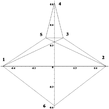
Figure 1: Mouse vertebra

Here we study three models, the Gaussian shape, and two shape Kotz type I models with $T=2$ and $T=3$.

First, the isotropic Gaussian shape density is obtained from corollary 5.1 when we set $R=\frac{1}{2}$, $\mathbf{\Sigma}=\sigma^{2}I_{N-1}$, $\mathbf{\Theta}=I_{K}$, $\mathbf{\Omega}=\mathbf{\Sigma}^{-1}\boldsymbol{\mu}\mathbf{\Theta}^{-1}\boldsymbol{\mu}^{\prime}=\sigma^{-2}\boldsymbol{\mu}\boldsymbol{\mu}^{\prime}$, namely

Corollary 6.1.

The Pseudo-Wishart reflection shape density based on the isotropic Gaussian is given by

$$dF_{\mathbf{W}}(\mathbf{W}) = \frac{\pi^{(nK-M)/2}|\mathbf{W}^{*}|^{(K-N)/2}J(\mathbf{u})\mathop{\rm etr}\nolimits\left(-\boldsymbol{\mu}^{\prime}\boldsymbol{\mu}/2\sigma^{2}\right)}{2^{-m+(-2+M+n(K-N))/2}\Gamma_{n}\left[K/2\right]}$$

$$\times\sum_{t=0}^{\infty}\frac{\Gamma\left[1+m+t+n(-K+N)/2\right]}{t!\sigma^{M-2-2m+n(K-N)}\left(\mathop{\rm tr}\nolimits\mathbf{W}\right)^{m-n(K-N)/2+t+1}}\sum_{\kappa}\frac{C_{\kappa}(\frac{1}{2\sigma^{2}}\boldsymbol{\mu}^{\prime}\mathbf{W}\boldsymbol{\mu})}{\left(\frac{1}{2}K\right)_{\kappa}}.$$

where $M=(N-1)K$.

A second shape distribution that we will use follows from corollary 5.2 by taking $R=1/2$, $T=2$, i.e.

$$dF_{\mathbf{W}}(\mathbf{W})=\frac{\pi^{(nK-M)/2}|\mathbf{W}^{*}|^{(K-N)/2}J(\mathbf{u})\mathop{\rm etr}\nolimits\left(-\boldsymbol{\mu}^{\prime}\boldsymbol{\mu}/2\sigma^{2}\right)}{2^{-2-m+(M+n(K-N))/2}M\Gamma_{n}\left[K/2\right]}$$

$$\times\sum_{t=0}^{\infty}\frac{(B-2t)\Gamma\left[a\right]+\Gamma\left[a+1\right]}{t!\sigma^{M-2-2m+n(K-N)}\left(\mathop{\rm tr}\nolimits\mathbf{W}\right)^{a}}\sum_{\kappa}\frac{C_{\kappa}(\frac{1}{2\sigma^{2}}\boldsymbol{\mu}^{\prime}\mathbf{W}\boldsymbol{\mu})}{\left(\frac{1}{2}K\right)_{\kappa}}.$$

where $M=(N-1)K$, $B=\mathop{\rm tr}\nolimits\boldsymbol{\mu}^{\prime}\boldsymbol{\mu}/2\sigma^{2}$ and $a=1+m+t+n(-K+N)/2$.

And the third shape model of this example corresponds to the isotropic Kotz distribution with $T=3$ and $R=1/2$, see (11).

In order to select the best elliptical model, a number of dimension criteria have been proposed. We shall consider a modification of the $BIC^{*}$ statistic as discussed in Yang and Yang (2007), and which was first achieved by Rissanen (1978) in a coding theory framework. The modified $BIC^{*}$ is given by:

$$BIC^{*}=-2\mathfrak{L}(\widetilde{\boldsymbol{\mu}},\widetilde{\sigma}^{2},h)+n_{p}(\log(n+2)-\log 24),$$

where $\mathfrak{L}(\widetilde{\boldsymbol{\mu}},\widetilde{\sigma}^{2},h)$ is the maximum of the log-likelihood function, $n$ is the sample size and $n_{p}$ is the number of parameters to be estimated for each particular shape density.

Now, if the goal of the shape analysis searches the best elliptical distribution, among a set of proposed models, the modified $BIC^{*}$ criterion suggests to choose the model for which the modified $BIC^{*}$ receives its smallest value. In addition, as proposed by Kass and Raftery (1995) and Raftery (1995), the following selection criteria have been employed in order to compare two contiguous models in terms of its corresponding modified $BIC^{*}$ .

Table 1: Grades of evidence corresponding to values of the $BIC^{*}$ difference.

$BIC^{*}$ difference	Evidence
0–2	Weak
2–6	Positive
6–10	Strong
$>$ 10	Very strong

Now, recall that for a general density generator $h(\cdot)$

$$\mathbf{X}\sim\mathcal{E}_{N\times K}(\boldsymbol{\mu}_{{}_{\mathbf{X}}},\mathbf{\Sigma}_{{}_{\mathbf{X}}}\otimes\mathbf{\Theta},h),$$

where $\boldsymbol{\mu}=\mathbf{L}\boldsymbol{\mu}_{{}_{\mathbf{X}}}$, then

$$\mathbf{Y}\sim\mathcal{E}_{N-1\times K}(\boldsymbol{\mu}\mathbf{\Theta}^{-1/2},\mathbf{\Sigma}\otimes\mathbf{I}_{K},h),$$

with $\mathbf{\Sigma}=\mathbf{L}\mathbf{\Sigma}_{\mathbf{X}}\mathbf{L}^{\prime}$.

In the mouse vertebra experiment, we want to find the maximum likelihood estimators (MLE) of the mean shape

$$\boldsymbol{\mu}=\left(\begin{array}[]{cc}\mu_{11}&\mu_{12}\\ \mu_{21}&\mu_{22}\\ \mu_{31}&\mu_{32}\\ \mu_{41}&\mu_{42}\\ \mu_{51}&\mu_{52}\\ \end{array}\right),$$

and the scale parameter $\sigma^{2}$ defined in the isotropy assumption $\boldsymbol{\Theta}=\mathbf{I}_{K}$ and $\boldsymbol{\Sigma}=\boldsymbol{\sigma}^{2}\mathbf{I}_{N-1}$, (in order to accelerate the computations of this example we fix the variance of the process as 50 -the maximum median variance of the two samples-). This optimisation is applied in the two independent populations, the small and large groups; first by assuming a Gaussian model and afterwards by considering two Kotz models indexed by $T=2$ and $T=3$.

The general procedure is the following: Let $\mathfrak{L}(\widetilde{\boldsymbol{\mu}},\widetilde{\sigma}^{2},h)$ be the log likelihood function of a given group-model. The maximisation of the likelihood function $\mathfrak{L}(\widetilde{\boldsymbol{\mu}},\widetilde{\sigma}^{2},h)$, is obtained in this paper by using the Nelder-Mead Simplex Method, which is an unconstrained multivariable function using a derivative-free method; specifically, we apply the routine fminsearch implemented by the sofware MatLab.

As the reader can check, the shape densities are series of zonal polynomials of the form

$$\sum_{t=0}^{\infty}\frac{f(t,\mathop{\rm tr}\nolimits\mathbf{X})}{t!}\sum_{\kappa}\frac{C_{\kappa}(\mathbf{X})}{(a)_{\kappa}},$$ (12)

which has hypergeometric series

$$\sum_{t=0}^{\infty}\frac{1}{t!}\sum_{\kappa}\frac{C_{\kappa}(\mathbf{X})}{(a)_{\kappa}},$$

as a particular case; these series were non computable for decades. The work of Koev and Edelman (2006) solved the problem and it let the computation of the hypergeometric series by truncation of the series until the coefficient for large degrees are zero under certain tolerance. The cited algorithm gives the coefficients of the series, then, we can modified the algorithm for hypergeometric series to compute the shape densities with the same computational costs, multiplying each coefficient of the series by the required function $f(t,\mathop{\rm tr}\nolimits\mathbf{X})$.

Table 2: The maximum likelihood estimators for the small group under the Gaussian model

Trunc.	$\widetilde{\mu}_{11}$	$\widetilde{\mu}_{12}$	$\widetilde{\mu}_{21}$	$\widetilde{\mu}_{22}$	$\widetilde{\mu}_{31}$	$\widetilde{\mu}_{32}$	$\widetilde{\mu}_{41}$
20	30.40	-8.13	5.73	9.47	4.01	17.34	-2.70
40	-0.47	-44.69	15.04	-4.54	25.27	0.60	4.88
60	-2.10	-54.84	18.31	-6.09	31.03	-0.12	6.17
80	-0.70	-63.48	21.37	-6.46	35.89	0.83	6.94
100	-2.61	-71.03	23.73	-7.85	40.19	-0.10	7.98
110	-0.54	-74.58	25.13	-7.50	42.16	1.14	8.12
120	-3.41	-77.44	25.88	-8.71	43.94	-0.37	8.79
140	-3.41	-77.44	25.88	-8.71	43.94	-0.37	8.79
160	-3.41	-77.44	25.88	-8.71	43.94	-0.37	8.79

Trunc.	$\widetilde{\mu}_{42}$	$\widetilde{\mu}_{51}$	$\widetilde{\mu}_{52}$	$BIC^{*}$	Time	Iter.
20	4.24	-6.82	-20.65	-3538.26	317	4103
40	5.21	-30.81	2.11	-4155.34	281	1881
60	6.23	-37.75	3.63	-4659.16	417	1923
80	7.40	-43.77	3.01	-5110.98	426	1455
100	8.08	-48.90	4.63	-5532.79	742	2025
110	8.72	-51.43	3.34	-5735.95	607	1507
120	8.76	-53.43	5.37	-5914.74	721	1640
140	8.76	-53.43	5.37	-5914.74	721	1640
160	8.76	-53.43	5.37	-5914.74	721	1640

Table 3: The maximum likelihood estimators for the small group under the Kotz $T=2$ model

Trunc.	$\widetilde{\mu}_{11}$	$\widetilde{\mu}_{12}$	$\widetilde{\mu}_{21}$	$\widetilde{\mu}_{22}$	$\widetilde{\mu}_{31}$	$\widetilde{\mu}_{32}$	$\widetilde{\mu}_{41}$
20	-6.06	-32.06	10.23	-5.19	18.24	-2.80	4.18
40	4.42	-46.00	15.97	-3.02	25.91	3.39	4.45
60	-0.53	-56.62	19.07	-5.73	32.01	0.80	6.18
80	-1.88	-65.36	21.89	-7.04	36.97	0.20	7.28
100	-0.04	-73.09	24.68	-7.18	41.31	1.40	7.90
110	-1.62	-76.63	25.72	-8.06	43.34	0.57	8.47
120	-1.84	-79.60	26.76	-8.39	45.13	0.56	8.83
140	-1.84	-79.60	26.76	-8.39	45.13	0.56	8.83
160	-1.84	-79.60	26.76	-8.39	45.13	0.56	8.83

Trunc.	$\widetilde{\mu}_{42}$	$\widetilde{\mu}_{51}$	$\widetilde{\mu}_{52}$	$BIC^{*}$	Time	Iter.
20	3.12	-21.88	5.46	-3584.58	311	1957
40	5.89	-31.91	-1.22	-4203.67	627	2052
60	6.61	-39.04	2.62	-4709.27	890	1986
80	7.49	-45.02	3.90	-5162.67	951	1566
100	8.60	-50.43	2.94	-5585.92	1468	1978
110	8.84	-52.81	4.17	-5789.74	1160	1386
120	9.18	-54.98	4.37	-5969.11	1464	1656
140	9.18	-54.98	4.37	-5969.11	1464	1656
160	9.18	-54.98	4.37	-5969.11	1464	1656

Table 4: The maximum likelihood estimators for the small group under the Kotz $T=3$ model

Trunc.	$\widetilde{\mu}_{11}$	$\widetilde{\mu}_{12}$	$\widetilde{\mu}_{21}$	$\widetilde{\mu}_{22}$	$\widetilde{\mu}_{31}$	$\widetilde{\mu}_{32}$	$\widetilde{\mu}_{41}$
20	-2.37	-33.66	11.14	-4.10	19.07	-0.68	3.91
40	-10.75	-46.42	14.62	-8.18	26.44	-5.17	6.28
60	-0.29	-58.24	19.64	-5.81	32.92	0.97	6.32
80	-1.69	-67.11	22.50	-7.15	37.96	0.35	7.45
100	-1.31	-74.91	25.17	-7.79	42.36	0.72	8.24
110	-1.33	-78.51	26.38	-8.15	44.39	0.77	8.64
120	-1.75	-81.49	27.42	-8.54	46.20	0.65	9.03
140	-1.75	-81.49	27.42	-8.54	46.20	0.65	9.03
160	-1.75	-81.49	27.42	-8.54	46.20	0.65	9.03

Trunc.	$\widetilde{\mu}_{42}$	$\widetilde{\mu}_{51}$	$\widetilde{\mu}_{52}$	$BIC^{*}$	Time	Iter.
20	3.71	-23.13	2.97	-3625.80	101	2083
40	4.30	-31.60	9.27	-4247.02	185	2067
60	6.82	-40.17	2.52	-4754.54	273	2050
80	7.72	-46.23	3.84	-5209.68	322	1816
100	8.68	-51.63	3.88	-5634.52	329	1449
110	9.10	-54.11	4.05	-5839.09	440	1776
120	9.41	-56.30	4.38	-6019.10	461	1688
140	9.41	-56.30	4.38	-6019.10	461	1688
160	9.41	-56.30	4.38	-6019.10	461	1688

Table 5: The maximum likelihood estimators for the large group under the Gaussian model

Trunc.	$\widetilde{\mu}_{11}$	$\widetilde{\mu}_{12}$	$\widetilde{\mu}_{21}$	$\widetilde{\mu}_{22}$	$\widetilde{\mu}_{31}$	$\widetilde{\mu}_{32}$	$\widetilde{\mu}_{41}$
20	-19.04	-22.88	5.37	-8.26	15.82	-10.82	3.84
40	-29.85	-29.93	6.54	-12.38	20.99	-17.32	5.62
60	-15.90	-49.41	14.07	-9.87	32.64	-7.20	5.30
80	-41.34	-43.55	9.73	-17.35	30.42	-23.86	7.93
100	-66.69	-8.40	-3.88	-21.92	9.43	-42.24	8.53
110	-40.91	-57.46	14.17	-18.57	39.32	-22.74	8.83
120	-32.30	-65.98	17.67	-16.67	44.17	-16.68	8.38
140	-32.30	-65.98	17.67	-16.67	44.17	-16.68	8.38
160	-32.30	-65.98	17.67	-16.67	44.17	-16.68	8.38

Trunc.	$\widetilde{\mu}_{42}$	$\widetilde{\mu}_{51}$	$\widetilde{\mu}_{52}$	$BIC^{*}$	Time	Iter.
20	1.42	-18.06	15.31	-3540.51	155	2075
40	1.52	-23.59	23.97	-4159.47	259	1824
60	4.80	-39.19	13.02	-4665.18	274	1295
80	2.35	-34.35	33.21	-5118.90	300	1044
100	-3.59	-6.20	53.12	-5542.62	978	2753
110	4.04	-45.42	32.97	-5746.72	449	1143
120	5.65	-52.16	26.15	-5926.64	509	1172
140	5.65	-52.16	26.15	-5926.64	509	1172
160	5.65	-52.16	26.15	-5926.64	509	1172

Table 6: The maximum likelihood estimators for the large group under the Kotz $T=2$ model

Trunc.	$\widetilde{\mu}_{11}$	$\widetilde{\mu}_{12}$	$\widetilde{\mu}_{21}$	$\widetilde{\mu}_{22}$	$\widetilde{\mu}_{31}$	$\widetilde{\mu}_{32}$	$\widetilde{\mu}_{41}$
20	-21.67	-21.97	4.83	-9.01	15.40	-12.56	4.10
40	-36.15	-24.57	4.23	-13.84	17.94	-21.68	6.00
60	-32.77	-42.35	10.19	-14.52	29.14	-18.44	6.82
80	-31.52	-53.20	13.74	-15.19	36.02	-16.98	7.42
100	-31.91	-61.32	16.28	-16.10	41.25	-16.74	8.02
110	-38.06	-61.70	15.79	-18.09	41.86	-20.66	8.78
120	-42.11	-62.61	15.65	-19.44	42.61	-23.16	9.32
140	-42.11	-62.61	15.65	-19.44	42.61	-23.16	9.32
160	-42.11	-62.61	15.65	-19.44	42.61	-23.16	9.32

Trunc.	$\widetilde{\mu}_{42}$	$\widetilde{\mu}_{51}$	$\widetilde{\mu}_{52}$	$BIC^{*}$	Time	Iter.
20	1.13	-17.32	17.40	-3586.83	339	2165
40	0.44	-19.28	28.94	-4207.80	476	1594
60	2.80	-33.46	26.38	-4715.29	519	1133
80	4.18	-42.10	25.47	-5170.59	706	1144
100	5.12	-48.56	25.83	-5595.75	1143	1528
110	4.74	-48.81	30.73	-5800.52	1105	1349
120	4.58	-49.41	33.92	-5981.01	1320	1459
140	4.58	-49.41	33.92	-5981.01	1320	1459
160	4.58	-49.41	33.92	-5981.01	1320	1459

Table 7: The maximum likelihood estimators for the large group under the Kotz $T=3$ model

Trunc.	$\widetilde{\mu}_{11}$	$\widetilde{\mu}_{12}$	$\widetilde{\mu}_{21}$	$\widetilde{\mu}_{22}$	$\widetilde{\mu}_{31}$	$\widetilde{\mu}_{32}$	$\widetilde{\mu}_{41}$
20	-31.74	3.30	-4.16	-9.72	-0.19	-20.55	3.56
40	-41.25	-18.15	1.70	-14.83	14.14	-25.34	6.17
60	-24.01	-49.58	13.33	-12.45	33.24	-12.39	6.27
80	-32.14	-54.75	14.17	-15.53	37.05	-17.29	7.60
100	-41.95	-57.11	13.96	-18.87	39.15	-23.43	8.93
110	-35.24	-65.37	17.23	-17.55	44.04	-18.63	8.70
120	-39.44	-66.43	17.11	-18.97	44.89	-21.22	9.27
140	-39.44	-66.43	17.11	-18.97	44.89	-21.22	9.27
160	-39.44	-66.43	17.11	-18.97	44.89	-21.22	9.27

Trunc.	$\widetilde{\mu}_{42}$	$\widetilde{\mu}_{51}$	$\widetilde{\mu}_{52}$	$BIC^{*}$	Time	Iter.
20	-2.58	2.86	25.23	-3628.05	73	1494
40	-0.67	-14.14	32.95	-4251.15	125	1411
60	4.26	-39.27	19.47	-4760.57	163	1239
80	4.32	-43.32	25.97	-5217.61	197	1110
100	3.93	-45.13	33.79	-5644.35	299	1345
110	5.37	-51.75	28.52	-5849.87	304	1246
120	5.21	-52.46	31.83	-6031.00	387	1457
140	5.21	-52.46	31.83	-6031.00	387	1457
160	5.21	-52.46	31.83	-6031.00	387	1457

At this point the log likelihood can be computed, then we use fminsearch for the MLE’s. The initial value for the algorithm is the sample mean of the elliptical matrix variables $\mathbf{Y}\sim\mathcal{E}_{N-1\times K}(\boldsymbol{\mu}\mathbf{\Theta}^{-1/2},\mathbf{\Sigma}\otimes\mathbf{I}_{K},h)$. However, we need to deal with an open problem proposed by Koev and Edelman (2006), the relationship between the convergence and the truncation of the series. Concretely, how many terms we need to consider in the series (12) in order to reach some fixed tolerance for convergence. A numerical solution consists of optimising the log likelihood, by increasing the truncation until, the MLE’s and the maximum of the function, reach an equilibrium, which depends on the standard accuracy and tolerance of the routine fminsearch. We tried the truncations $20,40,60,80,100,110,120,140$ and $160$, and we note that after the truncation 120 the solutions stabilise. the maximum likelihood estimators for location parameters associated with the small and large groups under the Gaussian, Kotz $T=2$ and Kotz $T=3$ models, are summarized in tables 2-7, respectively. Tables also show the modified $BIC^{*}$ value, the number of iterations for obtaining the convergence and the time in seconds for each optimisation.

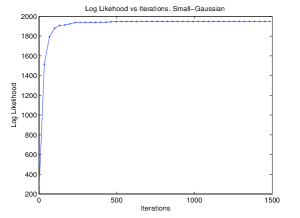
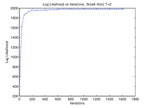
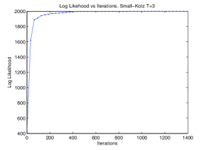
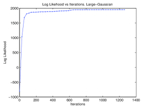
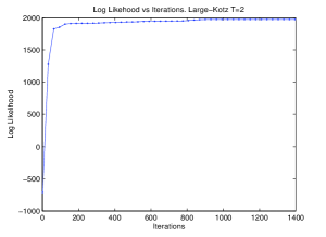
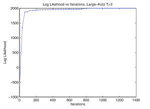
Figure 2: Behaviors of Log-Likelihood functions in terms of the iteration number of the fminsearch routine.

The computations were performed with a processor Intel(R) Corel(TM)2 Duo CPU, E7400@2.80GHz, and 2,96GB of RAM.

Figures 2 show the behavior of the maximum of the log likelihood when the number of iterations is increased. In this case we use a truncation of 160, and again, we note that the log likelihood is bounded for a very small number of iterations in each particular model.

According to the modified BIC criterion, we can order the models in the large and small groups as follows: (1) Kotz $T=3$, (2) Kotz $T=2$, (3) Gaussian.

This order can be seen in figure 3, which compares the log-likelihood of the two groups under the three models in terms of the algorithm iteration when the truncation is set in 160.

Modified $BIC^{*}$ of both groups shows a very strong difference (see table 1) between the best model (1) and the classical Gaussian (3).

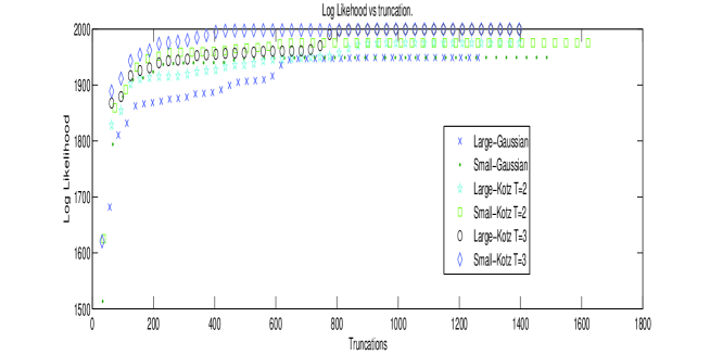
Figure 3: Comparison of Log-Likelihood in all models and groups in terms of the iteration number of the fminsearch routine.

In both cases, the true models of the data maybe have tails that are weighted more or less than Gaussian model or that the shape distribution present grater or smaller degree of kurtosis than the Gaussian model.

Remark 6.1.

We have used this example from the literature to illustrate the generalised shape theory; moreover, based on the modified $BIC^{*}$, we found that the Kotz distribution (with $T=3$) is the best model in this experiment. However, suppose the expert in the area of application knows that the landmarks have a Gaussian distribution, then we must apply the classical theory of shape (based on normality). Alternatively, if the expert in the application area suspects that the landmarks do not have a Gaussian distribution, so we can apply the generalized theory proposed here. In this case the expert has the necessary tools to choose an elliptical model (as an alternative to the Gaussian distribution), according to the characteristic of the sample which reveal and/or support a non Gaussian distribution, i.e. to select a distribution with more or less heavy tails, or more or less kurtosis than the Gaussian density; among many others possible characteristics.

Once the best models are selected for the small and large groups, we can test equality in mean shape between the two independent populations. In this experiment we have: two independent samples of 23 bones and 10 population shape parameters to estimate for each group. Namely, if $L(\boldsymbol{\mu}_{s},\boldsymbol{\mu}_{l})$ is the likelihood, where $\boldsymbol{\mu}_{s}$, $\boldsymbol{\mu}_{l}$, represent the mean shape parameters of the small and large group, respectively, then we want to test: $H_{0}:\boldsymbol{\mu}_{s}=\boldsymbol{\mu}_{l}$ vs $H_{a}:\boldsymbol{\mu}_{s}\neq\boldsymbol{\mu}_{l}$. Then $-2\log\Lambda=2\sup_{H_{1}}\log L(\boldsymbol{\mu}_{s},\boldsymbol{\mu}_{l})-2\sup_{H_{0}}\log L(\boldsymbol{\mu}_{s},\boldsymbol{\mu}_{l})$, and according to Wilk’s theorem $-2\log\Lambda\sim\chi^{2}_{10}$ under $H_{0}.$

Using fminsearch with a truncation of 160 we obtained that:

$$-2\log\Lambda=2(3999.1273)-2(3990.3601)=17.5344,$$

this is the same result when the series were truncated at 120 and 140. Since the p-value for the test is

$$P(\chi^{2}_{10}\geq 17.5344)=0.0633$$

we have some evidence that the small and large mouse vertebrae are different in mean shape. Mardia and Dryden (1989) studied this problem with a Gaussian model and Bookstein coordinates (see also Dryden and Mardia (1998)) and they obtained for the same test an approximate p-value of zero ($P(\chi^{2}_{8}\geq 127.75)$. Our test also rejects the equality of mean shape based on a better non Gaussian model but without an strong evidence as the Gaussian model suggests.

Note that the MLE’s given by tables 2-4 correspond to the matrix $\boldsymbol{\mu}$ in $\mathbf{Y}\sim\mathcal{E}_{N-1\times K}(\boldsymbol{\mu},\mathbf{\Sigma}\otimes\mathbf{I}_{K},h),$ we can use this information and the transformations

$$\mathbf{L}\mathbf{X}\mathbf{\Theta}^{-1/2}=\mathbf{L}\mathbf{Z}=\mathbf{Y}\Rightarrow\mathbf{V}=r\mathbf{W}=r\mathbf{W}(\mathbf{u}),$$

(with $\mathbf{V}=\mathbf{YY}^{\prime}$ and $\mathbf{W}=\mathbf{V}/r$) to estimate the different means at each step, i.e.: the original elliptical mean $\boldsymbol{\mu}_{\mathbf{X}}$, the size-and-shape mean $\boldsymbol{\mu}_{\mathbf{V}}$ and the shape mean $\boldsymbol{\mu}_{\mathbf{W}}$.

This example deserves a detailed study about some important facts, i.e. the distribution of $-2\log\Lambda$ for small samples, the truncation of the series, global optimisation methods, etc. These problems shall be considered in a subsequent work.

A final comment, for any elliptical model we can obtain the SVD reflection model, however a nontrivial problem appears, the $2t$-th derivative of the generator model, which can be seen as a partition theory problem. For the general case of a Kotz model ($s\neq 1$), and another models as Pearson II and VII, Bessel, Jensen-logistic, we can use formulae for these derivatives given by Caro-Lopera et al. (2009). The resulting densities have again a form of a generalised series of zonal polynomials which can be computed efficiently after some modification of existing works for hypergeometric series, see Koev and Edelman (2006), thus the inference over an exact density can be performed, avoiding the use of any asymptotic distribution, and the initial transformation avoids the invariant polynomials of Davis (1980), which at present are not computable for large degrees.

References

• Billingsley (1986) P. Billingsley, Probability and Measure, John Wiley & Sons, New York, 1986.
• Caro-Lopera et al. (2009) F. J. Caro-Lopera, J. A. Díaz-García and G. González-Farías, Noncentral elliptical configuration density, J. Multivariate Anal. 101(1) (2009), 32–43.
• Davis (1980) A. W. Davis, Invariant polynomials with two matrix arguments, extending the zonal polynomials, in: Multivariate Analysis V, (Krishnaiah, P. R. ed.), North-Holland, 1980.
• Díaz-García and Gutiérrez-Jáimez (1997) J. A. Díaz-García, and R. Gutiérrez-Jáimez, Proof of the conjectures of H. Uhlig on the singular multivariate beta and the jacobian of a certain matrix transformation, Ann. Statist., 25, (1997) 2018-2023.
• Díaz-García et al. (1997) J. A. Díaz-García, R. Gutiérrez-Jáimez, and K. V. Mardia, Wishart and Pseudo-Wishart distributions and some applications to shape theory, J. Multivariate Anal. 63 (1997) 73-87.
• Díaz-García and González-Farías (2005) J. A. Díaz-García and G. González-Farías, Singular random matrix decompositions: Distributions, J. Multivariate Anal. 194(1) (2005), 109–122.
• Díaz-García and Gutiérrez-Jáimez (2006) J. A. Díaz-García and R. Gutiérrez-Jáimez, Wishart and Pseudo-Wishart distributions under elliptical laws and related distributions in the shape theory context, J. Stat. Plan. Inference 136(12) (2006), 4176–4193.
• Dryden and Mardia (1998) I. L. Dryden and K.V. Mardia, Statistical shape analysis, John Wiley and Sons, Chichester, 1998.
• Fang and Zhang (1990) K. T. Fang, and Y. T. Zhang, Generalized Multivariate Analysis, Science Press, Springer-Verlag, Beijing, 1990.
• Goodall (1991) C. G. Goodall, Procustes methods in the statistical analysis of shape (with discussion), J. Roy. Statist. Soc. Ser. B, 53 (1991) 285-339.
• Goodall and Mardia (1993) C. R. Goodall, and K. V. Mardia, Multivariate Aspects of Shape Theory, Ann. Statist. 21 (1993) 848–866.
• Gupta and Varga (1993) A. K. Gupta, and T. Varga, Elliptically Contoured Models in Statistics, Kluwer Academic Publishers, Dordrecht, 1993.
• James (1964) A. T. James, Distributions of matrix variate and latent roots derived from normal samples, Ann. Math. Statist. 35 (1964) 475–501.
• Kass and Raftery (1995) R. E. Kass, and A. E. Raftery, Bayes factor, J. Amer. Statist. Soc. 90 (1995) 773–795.
• Khatri (1968) C. G. Khatri, Some results for the singular normal multivariate regression models, Sankhyā A 30 (1968) 267-280.
• Koev and Edelman (2006) P. Koev and A. Edelman, The efficient evaluation of the hypergeometric function of a matrix argument, Math. Comp. 75 (2006) 833–846.
• Le and Kendall (1993) H. L. Le, and D. G. Kendall, The Riemannian structure of Euclidean spaces: a novel environment for statistics, Ann.Statist. 21 (1993) 1225–1271.
• Mardia and Dryden (1989) K. V. Mardia and I. L. Dryden, The Statistical Analysis of Shape Data, Biometrika, 76(2) (1989) 271–281
• Muirhead (1982) R. J. Muirhead, Aspects of multivariate statistical theory, Wiley Series in Probability and Mathematical Statistics. John Wiley & Sons, Inc. 1982.
• Raftery (1995) A. E. Raftery, Bayesian model selection in social research, Sociological Methodology, 25 (1995) 111–163.
• Rao (1973) C. R. Rao, Linear Statistical Inference and its Applications (2nd ed.), John Wiley & Sons, New York, 1973.
• Rissanen (1978) J. Rissanen, Modelling by shortest data description, Automatica, 14 (1978) 465–471.
• Uhlig (1994) H. Uhlig, On singular Wishart and singular multivariate Beta distributions, Ann. Statist. 22 (1994) 395-405.
• Yang and Yang (2007) Ch. Ch. Yang and Ch. Ch. Yang, Separating latent classes by information criteria, J. Classification 24 (2007) 183–203.