Norm preserving stochastic field equation for an ideal Bose gas in a trap:
numerical implementation and applications

Abstract

Stochastic field equations represent a powerful tool to describe the thermal state of a trapped Bose gas. Often, such approaches are confronted with the old problem of an ultraviolet catastrophe, which demands a cutoff at high energies. In Hel09 we introduce a quantum stochastic field equation, avoiding the cutoff problem through a fully quantum approach based on the Glauber-Sudarshan $P$-function. For a close link to actual experimental setups the theory is formulated for a fixed particle number and thus based on the canonical ensemble. In this work the derivation and the non-trivial numerical implementation of the equation is explained in detail. We present applications for finite Bose gases trapped in a variety of potentials and show results for ground state occupation numbers and their equilibrium fluctuations. Moreover, we investigate spatial coherence properties by studying correlation functions of various orders.

I Introduction

The enormous progress in experimental and theoretical studies of ultracold quantum gases leads to a much deeper understanding of quantum many body physics Pet02 ; Pit03 ; Blo08 . In particular, Bose-Einstein condensation in traps enables us to investigate profoundly quantum statistical phenomena in finite systems. In more recent experiments, spatial and temporal coherences Blo00 ; Hel03 ; Foe05 ; Sch05 ; Oet05 of ultracold Bose gases are investigated in terms of correlation functions. Moreover, dynamics from nonequilibrium to equilibrium states Rit07 and the spatial dependence of equilibrium density fluctuations Est06 are considered. For a theoretical description of these phenomena it is desirable to consider nonzero temperature, finite size and – as no particle bath is present – a canonical description of the many-body quantum system. For most experiments, interaction between the atoms are of crucial importance. In systems with a Feshbach resonance, the interaction strength may even be tuned over a wide range – allowing to study ideal gases, too. In this article we deal almost exclusively with an ideal gas and comment on the interacting case briefly at the end of our paper.

It is clear that many properties of ultracold gases are sensitive to temperature not least due to the different size of the condensed fraction of the gas. Moreover, for these finite systems with a fixed number of particles, it is preferable to base a theoretical description on the canonical ensemble rather than the usual grand canonical ensemble. For an ideal gas, the best known example for the significance to choose the canonical ensemble is the fluctuation of the ground state occupation number $\langle N^{2}_{0}-\langle N_{0}\rangle^{2}\rangle$ Kac77 . Clearly, it approaches zero as temperature tends to zero in a canonical ensemble. Yet it is of the size of the average particle number $N$ in a grand canonical description. A detailed study of the fluctuations of the ground state particle number in the microcanonical and the canonical ensembles are given in Gro96 ; Pol96 ; Wil97 ; Gro97 ; Hol98 ; Koc00 . Spatial correlations are among other quantities of relevance for which a grand canonical formulation differs significantly from a canonical description Nar99 .

Recently, we presented a norm preserving stochastic field equation that describes the canonical state of an ideal Bose gas Hel09 . The resulting equation fully reflects quantum statistics and was given in Hel09 in a representation independent form. Therefore, it can be propagated in position space, meaning that it is not necessary to know eigenfunctions and -energies of the trapped atoms. While in Hel09 we simply state the equation and display a few applications, we here want to elaborate on its derivation, its numerical implementation and further applications in much more detail.

As we will show, spatial correlations and fluctuations can easily be calculated in position space. Due to the quantum framework, the equation – despite representing a c-number field – does not suffer from any cutoff problems which usually occur for classical field equations. Thus, numerical simulations can be performed with sufficient precision and reasonable effort.

Let us relate our approach to previous stochastic equations for the grand canonical ensemble. Note that most of these investigations are concerned with an interacting gas, while here, as a first step, we restrict ourselves to the case of the ideal gas. Since our theory can be formulated in position space, we clearly expect to be able to include interactions in a mean field sense in a next step.

Detailed discussions of different approaches to (interacting) ultracold gases in terms of stochastic field equations are given in Bra05 ; Pro08 . Exact methods based on the positive P-representation of the full density operator are used by Drummond and co-workers Dru04 . This theory brings about numerical challenges and is applied mainly to one-dimensional systems. More recently, also a 3D free gas at temperatures well below the transition temperature has been discussed Dru07 . Other approaches Sto97 ; Sto01 ; Dav01 ; Gar02 ; Bra05 can be seen as classical field methods, in which the lowly occupied energy levels must be treated in a different formalism or neglected, due to ultraviolet problems. Davis and co-workers apply a projection on a subspace of highly occupied energy levels, using a cutoff Dav01 , while Gardiner and co-workers separate the field operator in a highly and lowly occupied part Gar02 ; Bra05 . We see our approach more in the spirit of Stoof and co-worker, who start from a path integral approach and arrive at a functional Fokker-Planck equation for the Wigner functional of the thermal field Sto97 . After additional simplifications, in their work the corresponding Langevin equation takes the form of a classical stochastic field equation as given by Hohenberg and Halperin Hoh77 .

Apart from these grand canonical approaches, theories for a fixed particle number have also been presented more recently Xio02 ; Tri08 ; Tri082 ; Bar08 . Xu and co-workers describe Bose gases with first order perturbation theory and in a Bogoliubov approximation Xio02 . An exact phase-space description for a finite number of particles is worked out by Korsch and co-workers. Exact evolution equations for the Husimi-Q- and the Glauber-Sudarshan-P-distribution function based on a Bose-Hubbard Hamiltonian are derived Tri08 ; Tri082 . Stochastic methods in phase-space for the canonical ensemble of qubit and spin models have been presented by Drummond and co-workers Bar08 . While all these theories based on a canonical ensemble focus on different systems, e.g. lattices or spin models, we here aim to describe the full canonical thermal state of a Bose gas in any given trap.

Our novel equation presented in Hel09 has been found on the basis of the Glauber-Sudarshan-P-representation – being exact for an ideal gas. In this paper we aim to explain in more detail the derivation of the equation, its properties, its numerical implementation, and we show its power by discussing further applications. The paper is structured as follows: In the second section we show the theoretical background and the derivation of the stochastic field equation. The third section is devoted to the discussion of some crucial properties of the equation. In the fourth section we demonstrate how we propagate the equation in energy and in position space numerically. Results of these numerical applications are shown in the fifth section, before we draw conclusions in the final section.

II Stochastic field equation for the canonical ensemble

In order to derive a quantum stochastic field equation for the canonical ensemble of an ideal Bose gas, our first aim is to express quantum expectation values for a fixed particle number in terms of c-number integrals. The desired stochastic field equation should enable us to calculate these expectation values. We use the corresponding Fokker-Planck equation to demonstrate the equivalence of stochastic and canonical quantum ensemble mean.

We begin with the canonical density operator for $N$ particles

$$\hat{\rho}_{N}=\frac{1}{Z_{N}}e^{-\beta\hat{H}}P_{N}.$$ (1)

As usual, the Hamiltonian $\hat{H}=\sum\limits_{k}\epsilon_{k}\hat{a}^{\dagger}_{k}\hat{a}_{k}$ can be expressed in terms of occupation numbers of single-particle states ($\epsilon_{k}$ denotes the energy of single-particle state $k$). Furthermore, the canonical partition function is denoted by $Z_{N}$, with the usual $\beta=\frac{1}{kT}$ incorporating Boltzmann’s constant $k$ and temperature $T$. Crucially, a projector $P_{N}=\sum\limits_{\sum n_{k}=N}|\{n_{k}\}\rangle\langle\{n_{k}\}|$ on the $N$-particle subspace appears, with the usual number states $|\{n_{k}\}\rangle=\frac{1}{\sqrt{\prod\limits_{k}n_{k}!}}\prod\limits_{k}(\hat{a}^{\dagger}_{k})^{n_{k}}|0\rangle$. The operator $P_{N}$ projects the exponential $e^{-\beta\hat{H}}$ on a subspace of $N$ particles. In order to arrive at a c-number representation of quantum expectation values, one can express $e^{-\beta\hat{H}}$ from (1) as a mixture of coherent states using the (Glauber-Sudarshan) P-function representation Sch01

$$\frac{e^{-\beta\hat{H}}}{Z} = \frac{1}{\bar{n}}\int d\mu\{z\}\exp\left(-\sum\limits_{k}|z_{k}|^{2}(e^{\beta\epsilon_{k}}-1)\right)$$ (2)

$$\,\times|\{z\}\rangle\langle\{z\}|$$

$$= :\int d\mu\{z\}P(\{z\})|\{z\}\rangle\langle\{z\}|.$$

Here, we abbreviate the normalization factor with $\bar{n}=\prod\limits_{k}(e^{\beta{\epsilon_{k}}}-1)^{-1}$, and products of coherent states with $|\{z\}\rangle=|z_{0}\rangle|z_{1}\rangle\cdots|z_{n}\rangle\cdots$. The appropriate measure is $d\mu\{z\}=\prod\limits_{k}\left(\frac{d\{\text{Re}z_{k}\}d\{\text{Im}z_{k}\}}{\pi}\right)$.

Of particular interest are correlation functions of quantum field operators. Using the P-representation (2), we can determine canonical quantum expectation values with the help of $\langle\{z\}|P_{N}|\{z\}\rangle=\frac{1}{N!}(\sum\limits_{k}|z_{k}|^{2})^{N}e^{-\sum\limits_{k}|z_{k}|^{2}}$ (see Mol67 ) and obtain a weight function $W_{N}(\{z\})=\frac{1}{N!}\left(\sum\limits_{k}|z_{k}|^{2}\right)^{N}e^{\left(-\sum\limits_{k}|z_{k}|^{2}\right)}P(\{z\})$. With the latter, quantum expectation values can be written as integrals over c-numbers,

$$\langle\hat{a}^{\dagger}_{i}\hat{a}_{j}\rangle_{N}=\text{tr}\left(\hat{a}^{\dagger}_{i}\hat{a}_{j}\,\hat{\rho}_{N}\right)=\frac{1}{C}\int d\mu\{z\}z^{\ast}_{i}z_{j}W_{N-1}(\{z\})$$

(3)

with $C=\int d\mu\{z\}W_{N}(\{z\})$.

In this work we focus on spatial correlation functions. Therefore, we are interested in ensemble averages for the bosonic field operator $\hat{\psi}(x)=\sum\limits_{k}\langle x|\epsilon_{k}\rangle\hat{a}_{k}$ with $|\epsilon_{k}\rangle$ the single-particle eigenstate corresponding to energy $\epsilon_{k}$. First, the weight function is rewritten as $W_{N}(\{\psi\})=\frac{1}{N!}\left(\int dx\,|\psi(x)|^{2}\right)^{N}e^{\left(-\int dx\,|\psi(x)|^{2}\right)}P(\psi^{\ast},\psi)$ using $\psi(x)=\sum\limits_{k}z_{k}\langle x|\epsilon_{k}\rangle$ which is the eigenvalue of the field operator when applied to the coherent state $|\{z\}\rangle$, i.e. $\hat{\psi}(x)|\{z\}\rangle=\psi(x)|\{z\}\rangle$. Further, we obtain

$$\langle\hat{\psi}^{\dagger}(x)\hat{\psi}(x^{\prime})\rangle_{N} = \frac{1}{C}\int\,d\mu\{\psi\}\psi^{\ast}(x)\psi(x^{\prime})W_{N-1}(\{\psi\})$$

with the normalisation constant $C=\int d\mu\{\psi\}W_{N}(\{\psi\})$. It should be mentioned here that for quantum expectation values of second (or higher) order one has to use weight functions of different $N$. For $\langle\hat{\psi}^{\dagger}(x)\hat{\psi}^{\dagger}(x^{\prime})\hat{\psi}(x)\hat{\psi}(x^{\prime})\rangle$, for instance, the first order $W_{N-1}(\{\psi\})$ has to be replaced by $W_{N-2}(\{\psi\})$ – for higher orders the result changes accordingly (k-th order: chose $W_{N-k}(\{\psi\})$).

In order to calculate these expectation values we were able to construct a new, norm-preserving stochastic field equation Hel09 . The equivalence of quantum statistical and stochastic ensemble mean is based on the fact that the weight functions $W_{n}$ ($n=N,N-1,\ldots$) turn out to be stationary solutions of the corresponding Fokker-Planck equation.

In representation independent form ($\psi(x,t)=\langle x|\psi(t)\rangle$) and using Stratonovich calculus Gar83 it reads ($\hbar=1$ throughout)

$$\text{(S) }d|\psi\rangle=-\left((\Lambda+i)H-\Lambda\frac{\langle\psi|H|\psi\rangle}{\langle\psi|K|\psi\rangle}K\right)|\psi\rangle dt$$

$$+\sqrt{2\Lambda}\left(\sqrt{K}|d\xi\rangle-\frac{\langle\psi|\sqrt{K}|d\xi\rangle}{\langle\psi|K|\psi\rangle}K|\psi\rangle\right).$$ (5)

Here, the single particle Hamiltonian $H=\frac{p^{2}}{2m}+V(x)=\sum\limits_{k}\epsilon_{k}|\epsilon_{k}\rangle\langle\epsilon_{k}|$ appears, and a damping parameter $\Lambda$. Crucially, temperature enters through an operator

$$K=\frac{H}{e^{\beta H}-1}.$$ (6)

The noise increment $|d\xi\rangle$ is uncorrelated in space and time $\langle x|d\xi(t)\rangle\langle d\xi(t)|x^{\prime}\rangle=\delta(x-x^{\prime})dt$. Equation (II) is a norm preserving, non-linear stochastic equation that enables us to obtain canonical expectation values on average.

It is important to stress that the dependence of the stochastic fields $|\psi(t)\rangle$ on the particle number $N$ is indirectly given through their norm ${\cal N}=\langle\psi|\psi\rangle$ which is preserved during propagation and thus determined by the initial condition. One might expect ${\cal N}\approx N$ to be a reasonable choice; however, matters are more delicate and a distribution of norms ${\cal N}$ is required in order to obtain exact quantum expectation values. We devote the whole next Section III to the relation between norm ${\cal N}$ and particle number $N$.

Sometimes it useful to express (II) as an Ito-stochastic equation, reading

$$\text{(I) }d|\psi\rangle=-\left((\Lambda+i)H-\Lambda\frac{\langle\psi|H|\psi\rangle}{\langle\psi|K|\psi\rangle}K\right)|\psi\rangle dt$$

$$-\frac{\Lambda}{\langle\psi|K|\psi\rangle}\left(\text{tr}(K)-\frac{\langle\psi|K^{2}|\psi\rangle}{\langle\psi|K|\psi\rangle}\right)K|\psi\rangle dt$$

$$+\sqrt{2\Lambda}\left(\sqrt{K}|d\xi\rangle-\frac{\langle\psi|\sqrt{K}|d\xi\rangle}{\langle\psi|K|\psi\rangle}K|\psi\rangle\right).$$ (7)

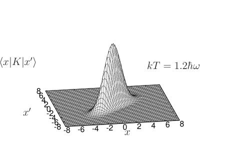
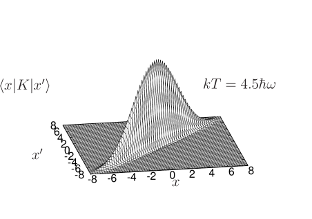
Figure 1: Correlation function $\langle x|K|x^{\prime}\rangle$ of the noise $|d\zeta\rangle=\sqrt{K}|d\xi\rangle$ of our stochastic field equation (II) for a harmonic potential. We show the correlation function for temperature $kT=1.2\hbar\omega$ (left) and for a higher temperature $kT=4.5\hbar\omega$ (right).

The novel stochastic field equation can be easily solved numerically and used in different representations. An implementation in the position representation is particularly useful as it can be applied to arbitrary external potentials $V(x)$. Based on the assumption of sufficient ergodicity, in applications the ensemble averages are replaced by a long time limit $\langle\hat{\psi}^{\dagger}(x)\hat{\psi}(x^{\prime})\rangle_{N}=\lim\limits_{t\rightarrow\infty}\frac{1}{t}\int\limits_{0}^{t}ds\,\{\psi^{\ast}(x,s)\psi(x^{\prime},s)\}$ over a single realization $\psi(x,s)$ of the stochastic field equation.

The term $(\Lambda+i)$ consists of a phenomenological damping term $\Lambda$, while ”$i$” describes ”real” dynamics. So, in a phenomenological manner, our equation can also be used to mimic the transition from a non-equilibrium to an equilibrium state.

It is important to point out the crucial role of the operator $K$. Its meaning becomes most apparent when we omit the nonlinear terms in our equation (II) and think of $H$ to represent $H-\mu$ which also affects the operator $K$. One obtains an equation which gives us the thermal state of the grand canonical ensemble Hel07

$$d|\psi\rangle=-(\Lambda+i)H|\psi\rangle dt+\sqrt{2\Lambda K}|d\xi\rangle.$$ (8)

with $\mu$ the chemical potential used to fix the average particle number $N$. It should be mentioned here that the canonical equation (II) is not merely a normalized version of the grand canonical equation. The linear equation (8) is closely related to the classical field equation for the thermal state of the grand canonical ensemble for any Hamiltonian energy functional ${\cal H}(\psi,\psi^{*})$ Hoh77

$$d\psi(x,t)=-(\Lambda+i)\frac{\delta{\cal H}}{\delta\psi^{*}}dt+\sqrt{2\Lambda kT}d\xi(x,t),$$ (9)

which has well-known ultraviolet problems. If one sets $\frac{\delta{\cal H}}{\delta\psi^{*}}=H\psi$, there is only one difference between classical (9) and quantum equation (8): the classical temperature $kT$ is substituted by the operator $K$. As discussed in Dav01 , for instance, the classical equation satisfies the equipartition theorem and therefore the infinite degrees of freedom of a field $\psi(x,t)$ lead to an ultraviolet catastrophe. This can also be seen in equ. (9) looking at a formulation in position space: the white noise term which is uncorrelated in position induces arbitrarily high momentum kicks. However, if we consider the operator $K=\frac{H}{e^{\beta H}-1}$ acting on the white noise $|d\xi\rangle$ in position space representation, the former white noise becomes spatially correlated, and we no longer get unphysical momentum. In other words, proper quantum statistics requires the replacement of spatially uncorrelated noise $\sqrt{kT}|d\xi\rangle$ in (9) by spatially correlated effective noise $|d\zeta\rangle=\sqrt{K}|d\xi\rangle$, as in (8). The correlation function of the effective noise $\langle x|d\zeta(t)\rangle\langle d\zeta(t)|x^{\prime}\rangle=\langle x|K|x^{\prime}\rangle\,dt$ is now a smooth function in position space and shown in Fig. 1 for two different temperatures.

In the low energy limit $H\ll kT$, indeed, the operator tends to the classical temperature $K\approx kT$. Yet in the case of high energies $H\gg kT$, the operator tends to zero $K\rightarrow 0$. We see that in the quantum equations (II, 8) the required cutoff is built in.

III Stochastic average and quantum expectation value

In this chapter we want to investigate the relationship between quantum expectation values of arbitrary order $\langle\hat{a}^{\dagger}_{i}...\hat{a}^{\dagger}_{j}\hat{a}_{k}...\hat{a}_{l}\rangle$ (3) and those obtained with the stochastic field equation (SFE) $\langle\langle z^{\ast}_{i}...z^{\ast}_{j}z_{k}...z_{l}\rangle\rangle_{\text{SFE}}$. For the following we introduce the norm ${\cal N}\equiv\sum\limits_{k}|z_{k}|^{2}=\langle\psi|\psi\rangle$ of the wavefunction. The stochastic equation keeps the norm fixed, while the integral of the quantum expectation values (3) extends over a range of values of the quantity $\sum\limits_{k}|z_{k}|^{2}$. The norm stays constant and for any stochastic method $\langle\langle 1\rangle\rangle_{\text{SFE}}=1$. Hence, we can write the first order expectation values we obtain from the stochastic equation as

$$\langle\langle z^{\ast}_{i}z_{j}\rangle\rangle_{\text{SFE}}({\cal N},\epsilon_{0})$$

$$\equiv\frac{\int d\mu\{z\}z^{\ast}_{i}z_{j}\delta({\cal N}-\sum\limits_{k}|z_{k}|^{2})W_{N-1}(\{z\})}{\int d\mu\{z\}\delta({\cal N}-\sum\limits_{k}|z_{k}|^{2})W_{N-1}(\{z\})}.$$ (10)

We find that this expression depends on the ground state energy $\epsilon_{0}$. It can be seen easily by a substitution $z\rightarrow ze^{\beta\epsilon_{0}/2}$ that the simple identity $e^{\beta\epsilon_{0}}\langle\langle z^{\ast}_{i}z_{j}\rangle\rangle_{\text{SFE}}({\cal N}e^{-\beta\epsilon_{0}},\epsilon_{0})=\langle\langle z^{\ast}_{i}z_{j}\rangle\rangle_{\text{SFE}}({\cal N},0)$ holds. The relation between the average values given by the stochastic field equation and quantum expectation values is now obvious

$$\langle\hat{a}^{\dagger}_{i}\hat{a}_{j}\rangle_{N} = \int d{\cal N}{\tilde{P}}({\cal N})\langle\langle z^{\ast}_{i}z_{j}\rangle\rangle_{\text{SFE}}({\cal N},\epsilon_{0}).$$ (11)

with the norm distribution

$${\tilde{P}}({\cal N})\equiv\frac{\int d\mu\{z\}\delta({\cal N}-\sum\limits_{k}|z_{k}|^{2})W_{N-1}(\{z\})}{\int d\mu\{z\}W_{N}(\{z\})}$$ (12)

in the integral (11).

Note that $\int d{\cal N}{\tilde{P}}({\cal N})=\int d\mu\{z\}W_{N-1}(\{z\})/\int d\mu\{z\}W_{N}(\{z\})\neq 1$. Therefore, and in order to get a better understanding of equ. (11), we have to investigate ${\tilde{P}}({\cal N})$ more closely. A lengthy calculation is given in appendix A, which results in

$${\tilde{P}}({\cal N})=\frac{1}{(N-1)!}\frac{{\cal N}^{(N-1)}\sum\limits_{k}c_{k}e^{-e^{\beta\epsilon_{k}}{\cal N}}}{\sum\limits_{k}c_{k}e^{-\beta\epsilon_{k}(N+1)}}.$$

with $c_{k}=\prod\limits_{\begin{array}[]{c}\scriptstyle l=0\scriptstyle\\ \scriptstyle l\neq k\end{array}}\left(e^{\beta\epsilon_{l}}-e^{\beta\epsilon_{k}}\right)^{-1}$. Well below the critical temperature it is sufficient to consider only the first term of the sum $\sum\limits_{k}c_{k}e^{-e^{\beta\epsilon_{k}}{\cal N}}$ because the remaining terms are smaller by a factor $e^{-(e^{\beta\epsilon_{k}}-e^{\beta\epsilon_{0}}){\cal N}}$. Numerical investigations of the factors $c_{k}$ showed that this approximation is justified in the temperature region considered here. Then our distribution ${\tilde{P}}({\cal N})$ is normalized to

$$\int\limits_{0}^{\infty}d{\cal N}{\tilde{P}}({\cal N})=\frac{\sum\limits_{k}c_{k}e^{-\beta\epsilon_{k}N}}{\sum\limits_{k}c_{k}e^{-\beta\epsilon_{k}(N+1)}}\approx e^{\beta\epsilon_{0}}.$$ (14)

Within this approximation we have a Poisson-like distribution

$${\tilde{P}}({\cal N})\sim{\cal N}^{(N-1)}\exp(-e^{\beta\epsilon_{0}}{\cal N}).$$ (15)

This distribution is centered around

$$\langle{\cal N}\rangle=\frac{\int\limits_{0}^{\infty}d{\cal N}{\tilde{P}}({\cal N}){\cal N}}{\int\limits_{0}^{\infty}d{\cal N}{\tilde{P}}({\cal N})}=Ne^{-\beta\epsilon_{0}}$$ (16)

and the standard deviation equals $\Delta{\cal N}=\sqrt{N}e^{-\beta\epsilon_{0}}$. For large $N$ the ratio of variance and mean goes to zero $\frac{\Delta{\cal N}}{\langle{\cal N}\rangle}\rightarrow 0$. Hence, in general it is sufficient to propagate equ. (II) with a single norm, i.e. we replace ${\tilde{P}}({\cal N})\approx e^{\beta\epsilon_{0}}\delta({\cal N}-Ne^{-\beta\epsilon_{0}})$. As a consequence, from (11) we get the simple relation $\langle\hat{a}^{\dagger}_{i}\hat{a}_{j}\rangle_{N}=e^{\beta\epsilon_{0}}\langle\langle z^{\ast}_{i}z_{j}\rangle\rangle_{\text{SFE}}(Ne^{-\beta\epsilon_{0}},\epsilon_{0})$ between canonical quantum correlation function and ensemble average of the stochastic field equation. As further elaborated upon in Section V, it is for very high precision only, that it is necessary to take into account the full norm distribution. Let us also remark that for higher order expectation values these considerations apply similarly.

It should be noted here that if the norm of our numerical simulation of the stochastic field equation ${\cal N}$ should correspond to the particle number $N$, we have to choose $\epsilon_{0}=0$. However, it is also possible to choose a norm different from the particle number according to (16). This freedom is useful for an easier numerical implementation, as shown in Section IV. It should also be mentioned that for temperatures above and near the critical temperature, the approximations leading to expression (14) are no longer valid and the exact norm distribution needs to be known. Still, using (14), for many quantities we observe satisfying results even in this temperature region.

IV Numerical implementation

In this section it is shown how one can solve the novel stochastic field equation numerically. The implementations can be done in different representations, whichever is convenient for a given trap potential. If the single particle eigenenergies are known (recall that we neglect interatomic interactions here) a propagation in energy space is the easiest way to solve our equation. In a box potential this is analogous to a propagation in momentum space. For a trap potential $V(x)$ with unknown energy spectrum, one can solve the equation in position space directly, using a split operator method based on Fast Fourier Transformation. This implementation is more challenging but the program can be easily adjusted to any trap just by changing the single line of code where the potential is defined.

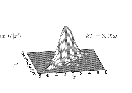
Figure 2: Correlation function $\langle x|K|x^{\prime}\rangle$ of the correlated noise of our stochastic field equation (II) for a harmonic potential at temperature $kT=3\hbar\omega$. We show the correlation function obtained from the noise in Wigner-Weyl approximation (left) compared to the exact result (right).

If the eigenvalues for the given trap potential are known, a numerical implementation in energy space does not contain any challenging aspects. As already explained above, it is more convenient to pass to position space, if we want to solve problems with arbitrary external potential, for which the eigenenergies are not known. We turn to a discretized formulation of equation (II) and use a position grid $\{x_{i}\}$ with some multi-index $i$. The part of the equation containing the single-particle Hamiltonian $H=\frac{p^{2}}{2m}+V(x)$ only can be propagated easily using standard Fast-Fourier transformation methods Fei82 .

The challenging aspect is the evaluation of matrix elements of the operator (6) appearing in (II), i.e. the determination of $\langle x_{i}|K|x_{j}\rangle=\left\langle x_{i}\left|\frac{\frac{p^{2}}{2m}+V(x)}{e^{\beta\left(\frac{p^{2}}{2m}+V(x)\right)}-1}\right|x_{j}\right\rangle$.

For an efficient implementation a Wigner-Weyl-approximation is helpful. The Wigner-Weyl correspondence Sch01 of the operator $K$ in $2D$-dimensional phase space is defined as

$$K(x,p)=\int d^{D}s\,e^{ips}\langle x+\frac{s}{2}|K|x-\frac{s}{2}\rangle,$$ (17)

with the help of which we can obtain the matrix elements as

$$\langle x_{i}|K|x_{j}\rangle=\frac{1}{(2\pi)^{D}}\int d^{D}p\,e^{ip(x_{i}-x_{j})}K\left(\frac{x_{i}+x_{j}}{2},p\right),$$

In order to simplify, we consider only zeroth order in $\hbar$, and find the classical expression

$$K(x,p)\approx\frac{\left(V(x)+\frac{p^{2}}{2}\right)}{e^{\beta\left(V(x)+\frac{p^{2}}{2}\right)}-1},$$ (19)

This approximation will be justified by comparing the approximated numerical result with exact numerical calculations.

Expanding the denominator in a geometric series we get

$$\langle x_{i}|K|x_{j}\rangle \approx \frac{1}{(2\pi)^{D}}\int d^{D}pe^{ip(x_{i}-x_{j})}\left(V\left(\frac{x_{i}+x_{j}}{2}\right)\right.$$ (20)

$$\left.\vphantom{\sum_{i=1}^{\lceil\frac{n}{2}\rceil}}+\frac{p^{2}}{2}\right)\sum\limits_{n=1}^{\infty}e^{-\beta n\left(V\left(\frac{x_{i}+x_{j}}{2}\right)+\frac{p^{2}}{2}\right)}$$

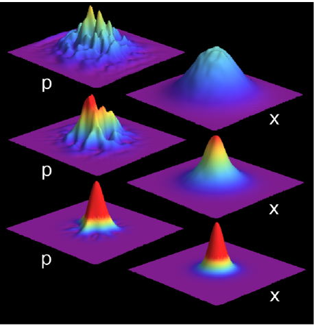
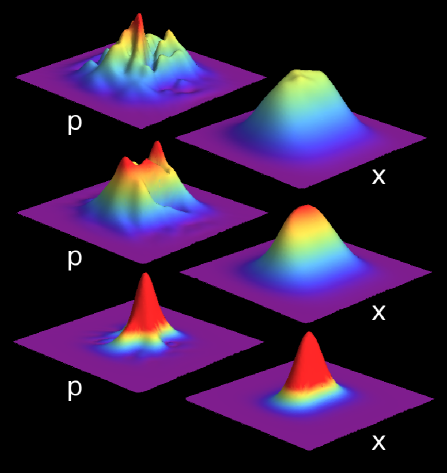
Figure 3: Wigner function of a Bose gas of $100$ particles trapped in a harmonic potential (left) and in the quartic potential $V(x,y,z)=x^{4}+y^{4}+z^{4}$ (right) above (top), at (middle), and below (bottom) the critical temperature. On the left hand side of both pictures we display a single realization with our stochastic field equation (II), on the right hand side a long-time average over 15000 time steps.
Top: almost a Boltzmann distribution for $T>T_{c}(N)$; middle: a peak develops for $T\approx T_{c}(N)$; bottom: almost all particles condense in the ground state, the Wigner function reflects the ground state Wigner function $T<T_{c}(N)$.

The momentum-integration can now be carried out without any difficulty which leads to the following expression:

$$\langle x_{i}|K|x_{j}\rangle \approx \frac{1}{(2\pi\beta)^{\frac{D}{2}}}\sum\limits_{n=1}^{\infty}e^{-\beta nV\left(\frac{x_{i}+x_{j}}{2}\right)}\left(V\left(\frac{x_{i}+x_{j}}{2}\right)\right.$$ (21)

$$\left.+\frac{D}{2\beta n}-\frac{(x_{i}-x_{j})^{2}}{2(\beta n)^{2}}\right)e^{\frac{-(x_{i}-x_{j})^{2}}{2\beta n}}.$$

It is important to note that the convergence of the geometric series in (20) very much depends on the minimum of the potential energy. Indeed, rapid convergence can be assured by adding some (physically irrelevant) constant to $V(x)$. However, as this shift also affects the ground state energy $\epsilon_{0}$, it also has a significant influence on the norm distribution of the wave function as can be witnessed in (16). Therefore, in practice one tries to identify some optimal shift that assures both, rapid convergence and a reasonable norm of the wave function.

An efficient generation of $\langle x_{i}|K|x_{j}\rangle$ is given in equ. (21). Now, in order to propagate equ. (II), it is necessary to think about the numerical implementation of the correlated noise $|d\zeta\rangle=\sqrt{K}|d\xi\rangle$, too. Obviously, the (discretized) noise $d\zeta_{i}=\langle x_{i}|d\zeta\rangle$ must be generated in a way that

$$d\zeta_{i}d\zeta_{j}^{*}=\langle x_{i}|K|x_{j}\rangle dt\\$$

holds. In order to find an efficient way to obtain the noise, we start with equ. (20). Based on the substitution $p\rightarrow\sqrt{n\beta}p$ we get

$$\langle x_{i}|K|x_{j}\rangle \approx \frac{1}{(2\pi\sqrt{n\beta})^{D}}\sum\limits_{n=1}^{\infty}e^{-\beta nV\left(\frac{x_{i}+x_{j}}{2}\right)}$$ (22)

$$\left(V\left(\frac{x_{i}+x_{j}}{2}\right)\int d^{D}pe^{i\frac{p(x_{i}-x_{j})}{\sqrt{n\beta}}}e^{-\frac{p^{2}}{2}}\right.$$

$$\left.\vphantom{\sum_{i=1}^{\lceil\frac{n}{2}\rceil}}+\frac{1}{n\beta}\int d^{D}p\frac{p^{2}}{2}e^{i\frac{p(x_{i}-x_{j})}{\sqrt{n\beta}}}e^{-\frac{p^{2}}{2}}\right).$$

For simplicity, the following derivation of an efficient noise generating method will be restricted to the one-dimensional case $D=1$. For higher dimensions, the strategy follows the very same lines.
The first integral $\int dpe^{i\frac{p(x_{i}-x_{j})}{\sqrt{n\beta}}}e^{-\frac{p^{2}}{2}}$ can be obtained from a Monte-Carlo integration of $\langle\!\langle e^{i\frac{\eta_{1}(x_{i}-x_{j})}{\sqrt{n\beta}}}\rangle\!\rangle$ over a normally distributed real random variable $\eta_{1}$. For the second momentum integral in (22), note that the integral $\int dp\frac{p^{2}}{2}e^{i\frac{p(x_{i}-x_{j})}{\sqrt{n\beta}}}e^{-\frac{p^{2}}{2}}$ can be seen as a radial integration in spherical coordinates according to

$$\int dp\frac{p^{2}}{2}e^{i\frac{p(x_{i}-x_{j})}{\sqrt{n\beta}}}e^{-\frac{p^{2}}{2}}=\int\limits_{0}^{\infty}dp\,p^{2}\cos\left(\frac{p(x_{i}-x_{j})}{\sqrt{n\beta}}\right)e^{-\frac{p^{2}}{2}}$$

$$=\frac{1}{4\pi}\int d^{3}{\bf p}\;\cos\left(\frac{\sqrt{p_{1}^{2}+p_{2}^{2}+p_{3}^{2}}(x_{i}-x_{j})}{\sqrt{n\beta}}\right)e^{-\frac{p_{1}^{2}+p_{2}^{2}+p_{3}^{2}}{2}}.$$

(23)

Obviously, now the integral in equ. (23) can be evaluated by a Monte-Carlo integration using three additional real Gaussian random numbers $\eta_{2},\eta_{3},$ and $\eta_{4}$. We arrive at the following representation of the correlation function as an average over four normally distributed real random variables $\eta_{1},\ldots,\eta_{4}$:

$$\langle x_{i}|K|x_{j}\rangle \approx \left\langle\frac{1}{(2\pi n\beta)^{\frac{1}{2}}}\sum\limits_{n=1}^{\infty}e^{-\beta nV\left(\frac{x_{i}+x_{j}}{2}\right)}\left(V\left(\frac{x_{i}+x_{j}}{2}\right)\right.\right.$$ (24)

$$\left.\times e^{i\frac{\eta_{1}(x_{i}-x_{j})}{\sqrt{n\beta}}}\right.$$

$$\left.+\frac{1}{2n\beta}\cos\left(\frac{\sqrt{\eta_{2}^{2}+\eta_{3}^{2}+\eta_{4}^{2}}x_{i}}{\sqrt{n\beta}}\right)\right.$$

$$\left.\cos\left(\frac{\sqrt{\eta_{2}^{2}+\eta_{3}^{2}+\eta_{4}^{2}}x_{j}}{\sqrt{n\beta}}\right)\right.$$

$$\left.+\frac{1}{2n\beta}\sin\left(\frac{\sqrt{\eta_{2}^{2}+\eta_{3}^{2}+\eta_{4}^{2}}x_{i}}{\sqrt{n\beta}}\right)\right.$$

$$\left.\left.\sin\left(\frac{\sqrt{\eta_{2}^{2}+\eta_{3}^{2}+\eta_{4}^{2}}x_{j}}{\sqrt{n\beta}}\right)\right)\right\rangle_{\eta}.$$

To proceed further we make use of the observation that the correlation function is very much concentrated along the diagonal $x=x^{\prime}$ (see Figs. 1,2). Based on this fact, we approximate $V\left(\frac{x_{i}+x_{j}}{2}\right)\approx\sqrt{V(x_{i})V(x_{j})}$ and $V\left(\frac{x_{i}+x_{j}}{2}\right)\approx\frac{V(x_{i})+V(x_{j})}{2}$, respectively, in order to achieve a factorization of the $x$-dependence on the right-hand-side in equ. (24). The final step is the introduction of a family of independent complex Wiener increments $d\kappa_{in}$ (with $i=1,2,3$ and $n=1,2,3,\ldots$), i.e. $d\kappa_{in}d\kappa^{*}_{jk}=\delta_{ij}\delta_{nk}dt$. With their help we achieve an explicit expression for the correlated noise in terms of independent Gaussian ($\eta$) and Wiener ($d\kappa$) random variables,

$$\langle x_{i}|\sqrt{K}|d\xi\rangle \approx \sum\limits_{n=1}^{\infty}\frac{e^{-\beta n\frac{V(x_{i})}{2}}}{(2n\beta\pi)^{\frac{1}{4}}}\left(\sqrt{V(x_{i})}d\kappa_{1n}e^{-i\frac{x_{i}\eta_{1}}{\sqrt{n\beta}}}\right.$$

$$\left.+\frac{1}{\sqrt{2n\beta}}\right.$$

$$\left.\times\left(d\kappa_{2n}\cos\left(\frac{x_{i}}{\sqrt{n\beta}}\sqrt{\eta_{2}^{2}+\eta_{3}^{2}+\eta_{4}^{2}}\right)\right.\right.$$

$$\left.\left.+d\kappa_{3n}\sin\left(\frac{x_{i}}{\sqrt{n\beta}}\sqrt{\eta_{2}^{2}+\eta_{3}^{2}+\eta_{4}^{2}}\right)\right)\right).$$

The good agreement of the correlation function of the noise in Wigner-Weyl approximation from (IV) and the exact correlation function can be seen in Fig. 2, where we show on the left an average over numerical realisations from (IV) and on the right the exact correlation function $\langle x_{i}|K|x_{j}\rangle$ for an isotropic harmonic oscillator at $kT=3\hbar\omega$.

To summarize this section, we are able to obtain the non-trivial noise and matrix elements of $K$ with reasonable effort. The other terms of the equation can be propagated using Fast-Fourier transformation. Thus, we are able to propagate the whole stochastic field equation in $D$ spatial dimensions. Results of such numerical simulations are presented in the following Section V.

V Results of numerical simulations

Our equation is here applied to a 3D Bose gas of fixed particle number trapped in various 3D potentials and different quantities are calculated. The results are obtained in energy or position representation. The applicability of our equation is first shown by determining the Wigner function $W(x,p)=\frac{1}{2\pi}\int dy\,e^{ipy}\langle\hat{\psi}^{\dagger}(x+\frac{y}{2})\hat{\psi}(x-\frac{y}{2})\rangle$ of a Bose gas. The propagation itself is performed in 3D position space, the figures show the Wigner function integrated over the remaining four phase space coordinates. As already explained in Section IV we use a Wigner-Weyl approximation for the simulation of (II).

In Fig. 3 we show the Wigner function for an ideal gas of $100$ particles for different temperatures and for an isotropic 3D harmonic potential (left) and the potential $V(x,y,z)=x^{4}+y^{4}+z^{4}$ (right). The left columns in both figures show a snapshot of a single realization, while the right columns display an averaged result over 15000 time steps. Clearly, to arrive at the equilibrium distribution, an average over many runs is required. The temperatures are chosen above, at, and below the critical temperature $T_{c}(N)$ (for the finite $N$ particle system). For the harmonic potential (left) one sees the expected qualitative properties; when applied to the potential $V(x,y,z)=x^{4}+y^{4}+z^{4}$ (right) we see that our implementation can be easily used for arbitrary trap potentials with an unknown energy spectrum.

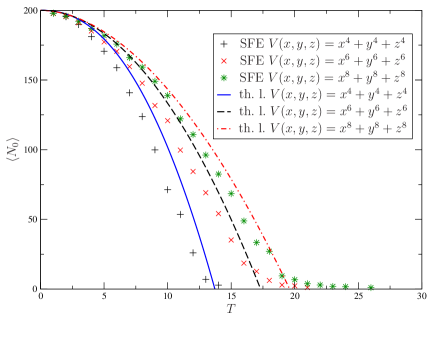
Figure 4: Ground state occupation as a function of temperature from a simulation of an ideal 3D Bose gas of 200 particles trapped in the potentials $V(x,y,z)=x^{4}+y^{4}+z^{4}$ (plus signs), $V(x,y,z)=x^{6}+y^{6}+z^{6}$ (crosses) and $V(x,y,z)=x^{8}+y^{8}+z^{8}$ (stars). We compare with the thermodynamic limit (full: $x^{4}$, dashed: $x^{6}$, dashed-dotted:$x^{8}$).

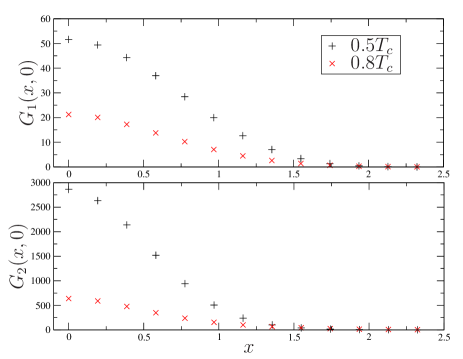
Figure 5: First and second order spatial correlations $G_{1}(x,0)$ (top) and $G_{2}(x,0)$ (bottom) obtained with our stochastic field equation for a Bose gas trapped in the potential $V(x,y,z)=x^{4}+y^{4}+z^{4}$ for different temperatures ($0.5T_{c}$: crosses, $0.8T_{c}$: stars).

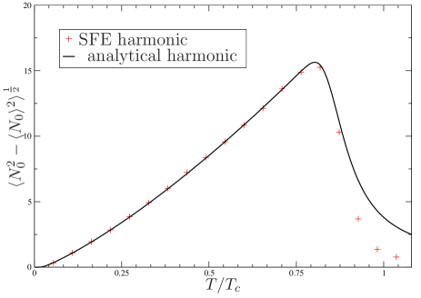
Figure 6: Simulation (plus signs) of the variance of the ground state occupation for a 3D ideal Bose gas in an isotropic harmonic potential compared to results from Koc00 (full line).

We next show that we also obtain good results quantitatively. First, we focus on the ground state occupation of the ideal gas. In Hel09 we showed the good agreement of our values with other canonical results for a box and a harmonic potential. In Fig. 4 results for the condensed fraction in potentials with higher powers than the harmonic case are shown. We use the 3D potentials $V(x,y,z)=x^{4}+y^{4}+z^{4}$ (plus signs), $V(x,y,z)=x^{6}+y^{6}+z^{6}$ (crosses) and $V(x,y,z)=x^{8}+y^{8}+z^{8}$ (stars) also to illustrate the flexibility of the numerical implementation of our equation. We compare with the results obtained in the thermodynamic limit (full line, dashed, dashed dotted); clearly, finite size effects are visible.

Spatial correlation functions are quantities which are often measured in experiments. In Hel09 we investigated second order correlation functions and their remarkable differences between a canonical and a grand canonical description. We also showed the good agreement of our values with corrected grand canonical results from Nar99 . Here we want to go beyond this well known results and show correlation functions for the potential $V(x,y,z)=x^{4}+y^{4}+z^{4}$. In Fig. 5 we present calculations of first $G_{1}(x,0)=\langle\hat{\psi}^{\dagger}(x)\hat{\psi}(0)\rangle$ and second order $G_{2}(x,0)=\langle\hat{\psi}^{\dagger}(x)\hat{\psi}^{\dagger}(0)\hat{\psi}(x)\hat{\psi}(0)\rangle$ correlation functions as they depend on the $x$-coordinate for a Bose gas of $200$ particles for temperatures below $T_{c}$ (plus signs, crosses).

The differences of the grand canonical and the canonical ensemble become very obvious when considering the fluctuations of the ground state occupation as a function of temperature. As already mentioned in the introduction, in a grand canonical description the variance for temperature near zero would be of the order of the particle number $N$. In Fig. 6 we display the ground state number fluctuations for a Bose gas of 200 particles in an isotropic harmonic potential in the canonical ensemble that clearly tend to zero as temperature lowers. We compare our calculation with the analytical canonical result of Koc00 which is based on the known eigenenergies for the harmonic potential.

So far, for the determination of the graphs in Figs. 3-5, is was sufficient to simulate with a single norm as elaborated upon in Sect. III. Now, we find that the number fluctuations are very sensitive with respect to slight errors of first $\langle N_{0}\rangle$ or second order $\langle N^{2}_{0}\rangle$ expectation values. Therefore, for this application, in order to reach the precision shown in Fig. 6, it is necessary to simulate with a distribution of norms. We use the simplified Poisson-type distribution from (15), which explains why near the critical temperature deviations from the exact result occur.

One can summarize our simulations by pointing out that with our stochastic field equation (II) in combination with the Wigner-Weyl approximation for the noise generation, one gets good numerical results for many different temperature dependent quantities in arbitrary potentials, also embracing the fixed particle number in these systems.

VI Conclusion and Outlook

In this paper we have discussed a novel stochastic field equation for a Bose gas with a finite and fixed particle number: our theory is based on the canonical ensemble referring to the conditions found in actual experiments with atomic gases in traps. The equation is exact for ideal gases. A generalization including atomic interactions appears possible on the basis of the inclusion of a mean-field interaction term in the potential.

Our approach to a numerical solution of the equation is explained in great detail. We focus on the implementation in position space, in which it is not necessary to know the single-particle eigenenergies of the system. By changing the specification of the external potential in the numerical code, we can easily determine equilibrium properties of the gas for many trap geometries. We can calculate correlation functions of arbitrary order and in principle obtain information about the full thermal canonical state. We show that it is possible to achieve results with satisfying precision for many different quantities of the ideal gas like first and second order correlation functions, ground state occupations and the variance of the ground state occupation.

VII Acknowledgement

We are grateful for inspiring discussions with Markus Oberthaler and Thimo Grotz. Sigmund Heller acknowledges support from the International Max Planck Research School for Dynamical Processes in Atoms, Molecules and Solids, Dresden.

Appendix A Calculation of the norm distribution ${\tilde{P}}({\cal N})$

In this appendix we derive expression (III) for the distribution of the norm,

$${\tilde{P}}({\cal N})=\frac{\int d\mu\{z\}\delta({\cal N}-\sum\limits_{k}|z_{k}|^{2})W_{N-1}(\{z\})}{\int d\mu\{z\}W_{N}(\{z\})},$$ (26)

with

$$W_{N-1}\{z\}=\frac{1}{(N-1)!}\left(\sum\limits_{i}|z_{i}|^{2}\right)^{N-1}e^{-\sum\limits_{i}e^{\beta\epsilon_{i}}|z_{i}|^{2}}.$$

which we use in Section III. Suppose the number of considered eigenstates equals $M$, which is arbitrary. We perform the transformation of variables: $|z_{i}|^{2}\rightarrow x_{i}$ and find

$$\tilde{P}({\cal N}) = \frac{2}{C}\int\limits_{0}^{\infty}d^{(M-1)}x\int\limits_{0}^{\infty}dx_{0}\delta(x_{0}-({\cal N}-\sum\limits_{i}x_{i}))$$ (28)

$$\frac{1}{(N-1)!}\left(\sum_{i}x_{i}\right)^{(N-1)}e^{-\sum\limits_{i}e^{\beta\epsilon_{i}}x_{i}}$$

$$= \frac{2}{C(N-1)!}{\cal N}^{(N-1)}e^{-e^{\beta\epsilon_{0}}{\cal N}}$$

$$\times\underbrace{\int\limits_{0<\sum\limits_{i=1}^{M-1}x_{i}<{\cal N}}d^{M-1}xe^{-\sum\limits_{i=1}^{M-1}(e^{\beta\epsilon_{i}}-e^{\beta\epsilon_{0}})x_{i}}}_{:=F_{M-1}}$$

with $C=\int d\mu\{z\}W_{N}(\{z\})$. First, we calculate the integral $F_{M}$.

$$F_{M} = \int\limits_{0}^{{\cal N}}dx_{1}\int\limits_{0<\sum\limits_{i=2}^{M-1}x_{i}<{\cal N}-x_{1}}dx_{2}...\int\limits_{0<x_{M}<{\cal N}-\sum\limits_{i=1}^{M-1}x_{i}}dx_{M}$$ (29)

$$\times e^{-\sum\limits_{i=1}^{M}(e^{\beta\epsilon_{i}}-e^{\beta\epsilon_{0}})x_{i}}.$$

Now we substitute $\tilde{x}_{1}=x_{1}$, $\tilde{x}_{2}=x_{2}+x_{1}$, $\tilde{x}_{3}=x_{3}+\tilde{x}_{2}$ etc. and rewrite the integral as

$$F_{M} = \int\limits_{0}^{{\cal N}}d\tilde{x}_{1}e^{-(e^{\beta\epsilon_{1}}-e^{\beta\epsilon_{2}})\tilde{x}_{1}}\int\limits_{\tilde{x}_{1}}^{{\cal N}}d\tilde{x}_{2}e^{-(e^{\beta\epsilon_{2}}-e^{\beta\epsilon_{3}})\tilde{x}_{2}}...$$ (30)

$$\int\limits_{\tilde{x}_{M-1}}^{{\cal N}}d\tilde{x}_{M}\,e^{-(e^{\beta\epsilon_{M}}-e^{\beta\epsilon_{0}})\tilde{x}_{M}}.$$

By considering a derivative with respect to ${\cal N}$ of equation (30) it can be seen that $F_{M}$ satisfies the differential equation

$$\frac{\partial F_{M}({\cal N})}{\partial{\cal N}}=e^{-(e^{\beta\epsilon_{M}}-e^{\beta\epsilon_{0}}){\cal N}}F_{M-1}({\cal N}).$$ (31)

We succeeded to find a solution with the ansatz

$$F_{M}({\cal N}) = \prod\limits_{k=1}^{M}\frac{1}{e^{\beta\epsilon_{k}}-e^{\beta\epsilon_{0}}}$$

$$+ \sum\limits_{k=1}^{M}\frac{g_{k}^{M}}{-e^{\beta\epsilon_{k}}+e^{\beta\epsilon_{0}}}e^{-(e^{\beta\epsilon_{k}}-e^{\beta\epsilon_{0}}){\cal N}}$$

with $g_{M}^{M}=\prod\limits_{k=1}^{M-1}\frac{1}{e^{\beta\epsilon_{k}}-e^{\beta\epsilon_{M}}}$ and $g_{k}^{M}=\frac{g_{k}^{M-1}}{-e^{\beta\epsilon_{k}}+e^{\beta\epsilon_{M}}}$. In this way we can obtain all coefficients $g_{k}^{M}$ iteratively. With a bit of analysis we find

$$F_{M}=\sum\limits_{k=0}^{M}\prod\limits_{\begin{array}[]{c}\scriptstyle l=0\scriptstyle\\ \scriptstyle l\neq k\end{array}}^{M}\frac{1}{(e^{\beta\epsilon_{l}}-e^{\beta\epsilon_{k}})}e^{-(e^{\beta\epsilon_{k}}-e^{\beta\epsilon_{0}}){\cal N}}.$$ (35)

Finally, we plug expression (35) into equation (28) and use $C=\int d\mu\{z\}W_{N}(\{z\})=\int d{\cal N}\int d\mu\{z\}\delta({\cal N}-\sum\limits_{k}|z_{k}|^{2})W_{N}(\{z\})$ to write the norm distribution in the form

$$\tilde{P}({\cal N})=\frac{1}{(N-1)!}\frac{{\cal N}^{(N-1)}\sum\limits_{k}c_{k}e^{-e^{\beta\epsilon_{k}}{\cal N}}}{\sum\limits_{k}c_{k}e^{-\beta\epsilon_{k}(N+1)}}.$$

with $c_{k}=\prod\limits_{\begin{array}[]{c}\scriptstyle l=0\scriptstyle\\ \scriptstyle l\neq k\end{array}}\frac{1}{(e^{\beta\epsilon_{l}}-e^{\beta\epsilon_{k}})}$, as it is written in equation (III) of Section III.

References

- (1) S. Heller and W. T. Strunz, J. Phys. B 42, 081001 (2009).
- (2) C. J. Pethick and H. Smith,Bose-Einstein Condensation In Dilute Gases (Cambridge University Press, Cambridge, 2002).
- (3) L. Pitaevskii and S. Stringari,Bose-Einstein Condensation(Oxford University Press, Oxford, 2003).
- (4) I. Bloch, J. Dalibard, and W. Zwerger, Rev. Mod. Phys. 80, 885 (2008).
- (5) I. Bloch, T. W. Hänsch and T. Esslinger, Nature 403, 166 (2000).
- (6) D. Hellweg, L. Cacciapuoti, M. Kottke, T. Schulte, K. Sengstock, W. Ertmer, and J. J. Arlt, Phys. Rev. Lett. 91, 010406 (2003).
- (7) S. Fölling, F. Gerbier, A. Widera, O. Mandel, T. Gericke, and I. Bloch, Nature 434, 481 (2005).
- (8) M. Schellekens, R. Hoppeler, A. Perrin, J. V. Gomes, D. Boiron, A. Aspect and C. I. Westbrook, Science 310, 648 (2005).
- (9) A. Öttl, S. Ritter, M. Köhl and T. Esslinger, Phys. Rev. Lett. 95, 090404 (2005).
- (10) S. Ritter, A. Öttl, T. Donner, T. Bourdel, M. Köhl and T. Esslinger, Phys. Rev. Lett. 98, 090402 (2007).
- (11) J. Esteve, J.B. Trebbia, T. Schumm,A. Aspect, C. I. Westbrook, and I. Bouchoule, Phys. Rev. Lett. 96, 130403 (2006).
- (12) M. Ziff, G. E. Uhlenbeck and M. Kac, Phys. Rep. 32, 169 (1977).
- (13) S. Grossmann, and M. Holthaus, Phys. Rev. E 54, 3495 (1996).
- (14) H. David Politzer, Phys. Rev. A 54, 5048 (1996).
- (15) M. Wilkens, and C. Weiss, J. Mod. Opt. 44, 1801 (1997).
- (16) S. Grossmann, and M. Holthaus, Phys. Rev. Lett. 79, 3557 (1997).
- (17) M. Holthaus, E. Kalinowski, and K. Kirsten, Ann. Phys. (N.Y.) 270, 198 (1998).
- (18) V. V. Kocharovsky, M. O. Scully, S.-Y. Zhu and M. S. Zubairy, Phys. Rev. A 61, 023609 (2000).
- (19) M. Naraschewski and R. Glauber, Phys. Rev. A 59, 4595 (1999).
- (20) A. S. Bradley, P. B. Blakies and C. W. Gardiner, J. Phys. B: At. Mol. Opt. Phys. 38, 4259 (2005).
- (21) N. P. Proukakis and B. Jackson, J. Phys. B 41, 203002 (2008).
- (22) P. D. Drummond, P. Deuar, and K. V. Kheruntsyan, Phys. Rev. Lett. 92, 040405 (2004); P. Deuar and P. D. Drummond, J. Phys. A 39, 1163 (2006); P. Deuar and P. D. Drummond, J. Phys. A 39, 2723 (2006); S. E. Hoffmann, J. F. Corney, and P. D. Drummond, Phys. Rev. A 78, 013622 (2008).
- (23) P. Deuar and P. D. Drummond, Phys. Rev. Lett. 98, 120402 (2007).
- (24) M. J. Davis, S. A. Morgan, and K. Burnett, Phys. Rev. Lett. 87, 160402 (2001); M. J. Davis, R. J. Ballagh, and K. Burnett, J. Phys. B: At. Mol. Opt. Phys. 34, 4487 (2001).
- (25) C. W. Gardiner, J. R. Anglin, and T. I. A. Fudge, J. Phys. B: At. Mol. Opt. Phys. 35, 1555 (2002).
- (26) H. T. C. Stoof, Phys. Rev. Lett. 78, 768 (1997);
- (27) R. A. Duine and H. T. C. Stoof, Phys. Rev. A 65, 013603 (2001).
- (28) P. Hohenberg and B. I. Halperin, Rev. Mod. Phys. 49, 435 (1977).
- (29) H. Xiong, S. Liu, G. Huang, and Z. Xu, Phys. Rev. A 65, 033609 (2002).
- (30) F. Trimborn, D. Witthaut, and H. J. Korsch, Phys. Rev. A 77, 043631 (2008).
- (31) F. Trimborn, D. Witthaut, and H. J. Korsch, Phys. Rev. A 79, 013608 (2009).
- (32) D. W. Barry and P. W. Drummond, Phys. Rev. A 78, 052108 (2008).
- (33) W. P. Schleich “Quantum Optics in Phase Space”, WILEY-VCH (2001).
- (34) B. R. Mollow, Phys. Rev. 168, 1896 (1967).
- (35) C. W. Gardiner “Handbook of Stochastical Methods”, Springer Verlag (1983).
- (36) S. Heller and W. T. Strunz, in “Path Integrals - new trends and perspectives” by W. Janke and A. Pelster (eds.), (World Scientific, Singapore, 2008).
- (37) M. D. Feit, F. A. Fleck, and A. Steiger, J. Comp. Phys., 47, 412 (1982).
- (38) K. Glaum, H. Kleinert and A. Pelster, Phys. Rev. A 76, 063604 (2007).