1 Introduction

A promising path for discoveries of TeV-scale particles to be produced at the LHC is through model-independent searches in which events can be classified in exclusive classes according to the number of identified high-$p_{T}$ objects (jets and leptons). In the case of heavy particles, with masses close to the TeV scale, the decay products undergo a significant Lorentz boost, and this leads to their partial or complete overlap. In the case of jets, this closes the opportunity of bump hunting in invariant-mass spectra using individual jets since the event signatures will be indistinguishable from those of the standard QCD-induced events.

Jet shapes are often discussed as a useful tool to disentangle events induced by the standard QCD processes from those containing jets as the results of decay products of TeV-scale particles. They are expected to be useful in reduction of the overwhelming rate of conventional QCD jets, thus opening the path to a direct observation of new states. [1, 2, 3, 4, 5, 6, 7, 8, 9, 10, 11, 12, 13, 14].

In this paper we extend the studies of jet shapes presented in [12] for the generic decay channel $X\to t\bar{t}\to hadrons$, with $X$ being a heavy particle with a mass close to the TeV scale. It is assumed that the mass of a particle $X$ is so heavy that the top quarks will form two energy deposits in cones around the top-quark directions. Thus, given the finite spacial resolution of a detector, the decay products of top quarks will be seen as monojets. It is hoped that shapes of such monojets will be different from those of the standard QCD jets, with direct implications for experimental searches of heavy particles.

While the approach presented in [12] was mainly based on two jet-shape variables, jet width and eccentricity derived using the principle-component analysis of jet constituents, in this paper we will propose a more intuitive approach which provides a significantly larger number of jet-shape characteristics. In fact, the approach proposed in this paper goes beyond the jet-shape identification and deals with a general problem of a dimensionality reduction, i.e. how to reduce the amount of information in the original multi-dimensional data keeping only a few parameters which catch the most basic spacial features of the original data. In the case of the jet-shape studies, we are interested not only in the extent of elongation of the jet shape characterized by the eccentricity, but also in a degrees of skewness of jet shapes which cannot be easily estimated using the techniques discussed before [12].

2 Jet shapes and jet masses

The jet-shape analysis performed in Ref. [12] included mass cuts and cuts on the jet shapes (the jet width and the eccentricity). The cut on the jet masses has by far the most rejection for QCD-jets. Indeed, the channel $X\to t\bar{t}\to hadrons$ features two monojets, each of which has a mass close to the top mass. Thus, selecting events with two jets with masses above some cut close to the top mass, one can reject a significant fraction of the standard QCD jets which have an exponentially decreasing mass spectra, unlike monojets from the top decays.

It has already been shown  [12] that there is a strong positive correlation between the jet mass and the jet width, thus applying cuts on jet mass and jet width at the same time may lead to unoptimized rejection factors. Therefore, in this paper we take a different approach and apply the mass cut before considering jet-shape variables. Table 1 shows the rejection factors after using the jet-mass cuts on two leading jets with $p_{T}>500$ GeV. The analysis was performed using the PYTHIA Monte Carlo model [15] included in the RunMC package [16] which interfaces FORTRAN Monte Carlo models with ROOT [17] and other C++ libraries. Jets and their shapes were reconstructed using the FastJet package [18]. The jets were reconstructed with the anti-$k_{T}$ algorithm [19] with a distance parameter of 0.6. Currently, this jet algorithm is the default for jet reconstruction at the ATLAS and CMS experiments. We simulated heavy-particle decays using $Z^{\prime}$ bosons as they are included in the PYTHIA model, forcing such states to decay to $t\bar{t}$ pairs. Both top quarks were set to decay hadronically. The PYTHIA parameters were set to the default ATLAS parameters tuned to describe multiple interactions [20]. The events were first generated and stored for easy processing.

Table 1 shows that the rejection factor after the jet-mass cut varies from $\sim 10$ to $\sim 400$ for the standard QCD events, while the mass cuts have a small effect on the events with TeV-scale particles, leading to a rejection between 1 and 2.3. For example, for the 70 GeV mass cut, the rejection factor for QCD events is roughly 9.9, while it is only a factor of $1.1$ for the 2 TeV signal events. Therefore, the ratio of the rejection factors for inclusive QCD and events with heavy states is about 9.

For the analysis of jet shapes in the next section, we will consider monojets with approximately similar masses, close to the top mass. We have chosen the jet-mass range $140<M(jet)<300$ GeV. With such a tight mass constraint, the jet shapes should mainly reflect the spacial distribution of jet constituents for kinematically similar jets (with similar transverse momenta and jet masses). Keeping this mass range in mind, we will attempt to find differences in jet shapes for QCD events and events originating from $X\to t\bar{t}\to hadrons$.

	$M(jet)>70$ GeV	$M(jet)>100$ GeV	$M(jet)>140$ GeV
$pp$	9.9	48	380
2 TeV	1.1	1.4	2.3
3 TeV	1.05	1.2	1.6
4 TeV	1.06	1.1	1.3

Table 1: Event rejection factors for inclusive $pp$ events and events with TeV-scale particles $Z^{\prime}\to t\bar{t}\to 6q$, where $Z^{\prime}$ has a mass ranging from 2 TeV to 4 TeV. The rejection factors were calculated by applying the cuts $70$, $100$ or $140$ GeV on the mass of two leading in $p_{T}$ jets.

3 Jet shapes using linear-regression analysis

To characterize jet shapes in two-dimensions, say in $\eta$ (pseudorapidity) and $\phi$ (azimuthal angle), we propose a new approach which is significantly different from the principle-component analysis considered in Ref. [12]. Being more intuitive, this method will also allow us to construct a significant number of jet-shape variables sensitive to the jet size in the transverse and longitudinal directions, as well as the degree to which the jet constituents form skewed shapes.

Let us consider a jet constituent (hadron, calorimeter cluster, etc.) defined by its position in $\eta$ (pseudorapidity) and $\phi$ (azimuthal angle) with respect to the beam-line and interaction-point, as well as by its energy $e$. In this case, each particle is represented by a point ($\eta$ and $\phi$) and a weight ($e$), making the shape effectively three-dimensional. If it is assumed that the jet in this phase space is a conic section (roughly elliptical), then we can define several shape variables, including the major axis length, minor axis length, ellipse eccentricity, and others (to be discussed below). The first task is thus to define the axes and lengths of the ellipse.

Figure 1: Sketch of two approaches for analyzing an approximately elliptical composite object. Each point represents a jet constituent, with the size representing its weight. The geometric major axis is defined by an unweighted linear regression, the geometric minor is by definition perpendicular to the major axis, through the geometric mean. In the non-quadrant method (left figure), weighted centers P[N] ($N=1,\ldots,4$) are defined for the regions above or below the major and minor axes. In the quadrant-method (right figure), each weighted center P[N] is uniquely associated with one of four quadrants shown with dashed lines and denoted as (1)-(4). In both methods, the weighted centers do not need to be located on the axes.

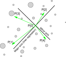
First, a linear regression analysis in two-dimensions is performed to define the direction of geometrical elongation in $\eta$ and $\phi$. The linear regression was performed using the least squares approach by minimizing the sum of the squares of the vertical distances of the points from the line. At this stage, all data points are assumed to have exactly the same weights. The linear regression defines the best-fit values of the slope and intercept of the major axis. In the calculations, a geometric mean of all constituents is found first (P[0] in Fig. 1) and then a linear regression is performed. The major axis is given by the fit, while the minor axis is defined to be perpendicular to the major axis and passing through the geometric mean.

With the axis-lines of the ellipse defined, the next step is to calculate the axis length. We identified two main classes of length definition: the quadrant method and the non-quadrant method. We will discuss each of these methods respectively.

3.1 Quadrant Method (QM)

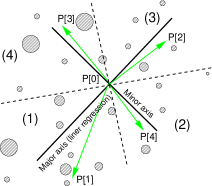
In the quadrant method (QM), the $\eta-\phi$ space is first divided into four quadrants centered at the ellipse geometric center, each of which corresponds to one of the ellipse semi-axes (Fig. 1 (right)). This is done by taking the major and minor axis lines (from linear regression) and rotating them by $45^{o}$, putting each semi-axis in one of the quadrants, as this shown using dashed lines in Fig. 1(right). The length of each semi-axis is defined by finding the weighted center of each quadrant; that is, all constituent points are separated by the quadrant in which they lie and the weighted mean of each quadrant is found independently, without consideration of points in other quadrants. Each data point is uniquely associated with each quadrant. The length of the semi-axis is thus the length between the global geometric center and the quadrant center.

The semi-axes are sensitive to spacial positions of jet constituents in 3D (where the third component, the constituent weight, is given by energy), since the geometrical axes are defined using unweighted regression, while the semi-axes are calculated using weights.

3.2 Non-Quadrant Method (NQM)

In the non-quadrant method (NQM), the major and minor axis themselves define the areas where the weighted means are calculated; the major axis-line defines two semi-planes (the part above and the part below), as does the minor axis-line, see Fig. 1(left). In this way, each point is in two of four semi-planes rather than a single exclusive quadrant. The weighted means above and below the major axis-line are the weighted centers defining the lengths of the minor semi-axes, while the means above and below the minor axis define the lengths of the major semi-axes.

As example, the point P[3] in Fig. 1(left) shows a weighted mean of the area above the major axis, while P[4] defines the same but for the plane below the major axis. Similarly, [P1] and P[2] show the weighted means for the plane below and above the minor axis. It is important to note that all four centers are defined using weights (i.e. jet constituent energies), which increase the sensitivity to data in 3D. The distances between the points P[1] and P[0] (P[2] and P[0]) define major semi-axes. Analogously, the distances between the points [P3] and P[0] ([P4] and P[0]) define the minor semi-axes.

The main difference between the QM and NQM is different sensitivity to spacial topology: Each point in the NQM contributes to both major and minor semi-axes. Thus, the NQM is more sensitive to a shape of elongated distribution, since all points from both sides of the major axis contribute to the (semi)-minor length. For example, a shape with roughly the same width along the major axis (a pencil-like shape) indicates a very small minor length.

For the QM method, points are uniquely associated with each quadrant and can contribute either to the minor or the major semi-axis. In the example with a pencil-like shape discussed above, only a small fraction of phase space close to the geometrical center can contribute to the minor axis. Adding an extra point in the region of $45^{o}$ from one side of the major axis will have a strong impact on the minor semi-axis, without contribution to the major semi-axis (unlike the NQM definition).

3.3 Definition of Variables

The geometrical major and minor axes from the linear-regression analysis were only necessary to define the regions with four positions of semi-axes which are used for calculations of actual major and minor vectors and jet-shape variables based on these vectors. Each variable can be defined either in QM or NQM.

• Major length, $|\vec{L}_{MJ}|$, a distance between major semi-axis centers (P[1] and P[2]) which defines the size of longitudinal elongation (which includes 2D geometry and weights given by the energies of constituents). It can be composed into two semi-axes from each side of the minor axis. By definition, $\vec{L}_{MJ}=\vec{L}_{MJ}^{(1)}-\vec{L}_{MJ}^{(2)}$ and $|\vec{L}_{MJ}^{(1)}|>|\vec{L}_{MJ}^{(2)}|$, where $|\vec{L}_{MJ}^{(1)}|$ is the longest and $|\vec{L}_{MJ}^{(2)}|$ shortest length of the semi-axis.

• Minor length, $|\vec{L}_{MI}|$, a distance between minor semi-axis centers (P[3] and P[4]) which defines the size of the transverse elongation. It can be decomposed into two semi-axes from each side of the major axis. By definition, $\vec{L}_{MI}=\vec{L}_{MI}^{(1)}-\vec{L}_{MI}^{(2)}$ and $|\vec{L}_{MI}^{(1)}|>|\vec{L}_{MI}^{(2)}|$, where $\vec{L}_{MI}^{(1)}$ is the longest and $|\vec{L}_{MI}^{(2)}|$ the shortest length of the minor semi-axis.

• Eccentricity, $ECC$, defined as

  $$ECC=1-\frac{|\vec{L}_{MI}|}{|\vec{L}_{MJ}|}$$

  with the range $[0,1]$. This variable measures the degree to which the ellipse fails to be circular. $ECC=0$ is for a perfect circle, and 1 for an infinitely elongated object. For the QM, this parameter emphasizes the relative width of an elongated object due to contributions of points closer to the geometrical center, while the same parameter in the NQM is more sensitive to the contribution of points away from the center.

• Major eccentricity, $ECC_{MJ}$:

  $$ECC_{MJ}=1-\frac{|\vec{L}_{MJ}^{(2)}|}{|\vec{L}_{MJ}^{(1)}|},$$

  where $|\vec{L}_{MJ}^{(1)}|$ and $|\vec{L}_{MJ}^{(2)}|$ are the lengths of the major semi-axes as defined above. This is a measure of the degree to which the ellipse is skewed to one side of the minor axis. A large value signifies a large difference between lengths of the major semi-axes. For the QM, it is sensitive to skewness due to points close to the geometrical center, while for the NQM it is more sensitive to points at the shape edges.

• Minor eccentricity, $ECC_{MI}$:

  $$ECC_{MI}=1-\frac{|\vec{L}_{MI}^{(2)}|}{|\vec{L}_{MI}^{(1)}|},$$

  where $|\vec{L}_{MI}^{(1)}|$ and $|\vec{L}_{MI}^{(2)}|$ are the lengths of the minor semi-axes. This is a measure of the degree to which the ellipse is ’skewed’ to one side of the major direction. A large value signifies a large difference between lengths of the minor semi-axes. As before, the value of $ECC_{MI}$ is in the range [0,1]. The differences between the QM and NQM methods are as for the $ECC_{MJ}$.

The above variables can be defined using either the QM or NQM. As mentioned above, the QM is sensitive to the asymmetries in the shape close to the geometrical center of the entire distribution, while the NQM is more sensitive to asymmetry at the edges.

Figure 2: Several examples illustrating the concept of the shape-variables in the linear-regression approach. 400 points in $\eta$ and $\phi$ phase space are distributed randomly using two overlapping Gaussian distributions: (1) the mean positions of the Gaussian distributions are the same; (2) two Gaussian distributions are shifted by 3 (arbitrary) in $\eta$-direction; (3) the same as before, but a new point was added with the weight 50 (open circle); (4) the heavy-weight point was moved closer to the major axis. The thick (red) line shows the linear regression which defines the major axis, while thin black line is the minor axis. The eccentricities are calculated using the NQM and QM as described in the text.

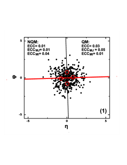
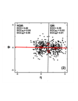
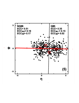
To illustrate the concept of the linear-regression approach, numerical tests were performed by distributing random points in 2D using two Gaussian distributions, see Fig. 2. The thick (red) line shows the linear regression which defines the geometric major axis, while the thin black line is the geometric minor axis. The eccentricities were calculated using the NQM and QM. The following situations were considered: (1) the mean positions of the Gaussian distributions were set to be the same. (all eccentricities are close to zero); (2) the centers of two Gaussian distributions were shifted by 3 units in $\phi$-direction. This leads to non-zero global eccentricities, and the eccentricities which reflect skewness ($ECC_{MJ}$ and $ECC_{MI}$) are close to zero. When a new point is added with the weight 50 (open circle) (see Fig. 2(3)), this impacts the values of $ECC_{MI}$. Moving this point closer to the major axis (Fig. 2(4)) changes the value of $ECC_{MJ}$.

Figure 3 shows the variables for the signal and background events for the leading in $p_{T}$ jet, after the mass cuts at $140$ GeV as discussed in Sect. 2. For a better shape comparison, all distributions are normalized to unity. It should be stressed that, in reality, the cross sections for QCD events can be three orders of magnitude larger than those for the signal events. We will discuss this point later; at this stage we are only interested in the shape comparison.

As it can be seen from Figure 3, the mass cut is essential for the TeV-scale particle searches: in addition to the fact that it is strongest for separation of background events, the differences between jet shapes for the signal and background events significantly depend on the applied mass cut. Similarly, Fig. 4 shows the same variable but for the second jet.

Arrows on Figures 3 and 4 show possible cuts designed to reject QCD events in $pp$ collisions. The mass cut is applied for all shape distributions. It should be noted that cuts on the shape variables are applied after using the other cuts (indicated on the figure). We did not apply the cuts on the eccentricities in the NQM approach since a cut on the $|\vec{L}_{MI}^{NQM}|$ is already sufficient to make sure that only asymmetric events are accepted. It can be seen that the jet-shape cuts should be tightened for 3 and 4 TeV particles to obtain the largest possible rejection for QCD jet events.

Figure 3: Jet mass and jet-shape variables for the leading in $p_{T}$ jet in inclusive $pp$ collisions (filled histograms) simulated with the PYTHIA model. The jet shapes are shown after using the jet-mass cut $M(jet)>140$ GeV. Also shown are the shape variables for $X\to t\bar{t}\to W^{+}b_{1}W^{-}b_{2}$, with $W$ bosons decaying hadronically into two jets. The state $X$ was simulated using a $Z^{\prime}$ particle with a mass of $2$, $3$ and $4$ TeV (solid and dashed lines, respectively). Events were selected with at least one jet with $p_{T}>500$ GeV using the anti-$k_{T}$ jet algorithm. The vertical lines show the cuts applied to reject inclusive QCD events.

Figure 4: Same as Fig. 3, but for the second leading in $p_{T}$ jet.

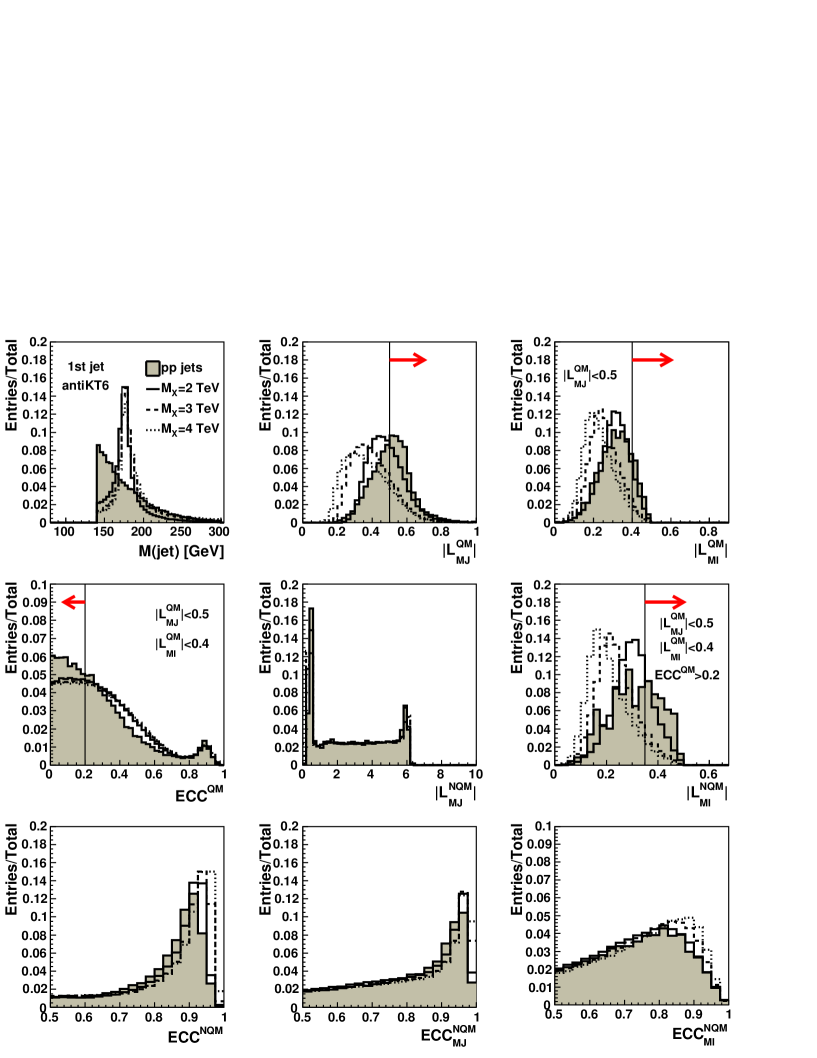
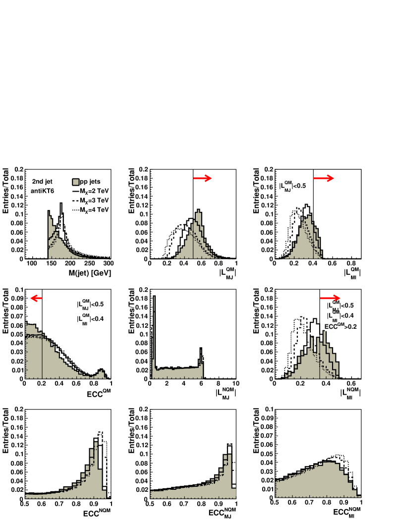
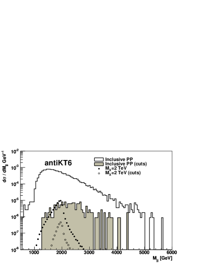
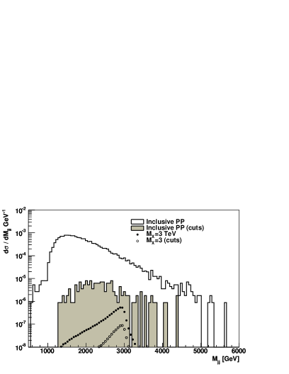
Figure 5 shows the expected differential cross sections for the jet-jet invariant mass $M_{jj}$ after the mass cut $M(jet)>140$ GeV. The distributions are shown before and after the applied jet-shape cuts indicated with the arrays in Fig. 3 and 4. It can be seen that after the jet-shape cuts, the expected signal (open dots) is a factor of ten smaller than the QCD background level (the filled histograms), while it is much larger for the jet-mass cut alone (filled dots and the open histogram). Certainly, the conclusion about the relative size of the signal compared to QCD background depends on the underlying model, which, in this case, was chosen to be the $Z^{\prime}$. The relative size of the signal compared to QCD background does not change much with increase of $M_{X}$, which is mainly due to the fact that no readjustments of the jet-shape cuts were done going to higher masses.

Let us give numerical estimates. The rejection factor $r(QCD)$ for QCD events in the mass range $1.5-2.5$ TeV is roughly $100$, while it is a factor $25$ for the 2 TeV signal. Therefore, the ratio of the rejection factors for inclusive QCD and events with heavy states is about $3.7$,

$$\frac{r(QCD)}{r(X(2TeV))}\simeq 3.7.$$ (1)

The rejection factor for QCD events for $M_{jj}\sim 2$ TeV is $44$, while it is only a factor $7.4$ for 3 TeV particles. Therefore, the ratio of the rejection factors for inclusive QCD and events with 3 TeV states is larger:

$$\frac{r(QCD\>\>jets)}{r(X(2\>\>TeV))}\simeq 6.$$ (2)

For the 4 TeV signal events, the rejection can be as high as 8 after adjusting the cuts on the shape variables. Generally, it is expected that the relative rejection factor will be even larger for higher masses and roughly follows:

$$\frac{r(QCD\>\>jets)}{r(X(M\>\>TeV))}\propto M,$$ (3)

where $M$ is a mass (in TeV) of a heavy particle. At this stage, it is difficult to verify the exact functional dependence on $M$ since this depends on the chosen jet-shape cuts. We only can offer an approximate dependence which qualitatively follows from Figs. 3 and 4.

Using the jet-shape rejection rates, now it is easy to calculate the global rejection factor including the jet-mass cut. We will make our estimates for the 3 TeV exotic particles. According to Table 1, the relative rejection factor for 140 GeV mass cut is 380/1.6=237. The rejection factor only weakly depends on the mass of heavy particles after using the jet-mass cut to consider only jets with masses close to the nominal top mass. This rejection factor should be multiplied by the factor Eq. (2) from the use of jet-shape variables. Thus, the overall relative rejection factor is above 1400.

For an arbitrary TeV-scale mass $M$ of a heavy state decaying to $t\bar{t}$, the total relative rejection factor follows this empirical expression:

$$\frac{r_{tot}(QCD\>\>jets)}{r_{tot}(X(M\>\>TeV))}\simeq C\cdot(A+M),$$ (4)

where an $C$ is a rejection factor which significantly depends on the mass cuts as shown in Table 1, but relatively independent of the heavy-state mass. The second factor, $A+M$ (with $A$ being a constant) originates from the jet-shape selection and explicitly depends on the mass of a heavy state.

Figure 5: The differential cross section for the jet-jet invariant mass after the mass cut $M(jet)>140$ GeV before (open histograms and filled symbols) and after (filled histogram and open symbols) the jet-shape cuts. We used the PYTHIA model for the simulation of $Z^{\prime}$ particles with 2, 3 and 4 TeV masses. The relative size of the signal compared to the QCD background level increases after applying the jet-shape cuts. See the text for more detailed numerical estimates.

The efficiency of the selection of new states significantly depends on the applied cuts and the mass of such states. For the example discussed above, the overal efficiency including the applied mass cuts is roughly $8\%$ for a $X$ state with the mass 3 TeV.

Since the anti-$k_{T}$ jet algorithm turns out to produce circular shapes [19], it is likely that the use of other jet algorithms may lead to different rejection factors obtained using the jet shapes. In particular, we expect that the standard $k_{T}$ algorithm [23] with a larger cone size (0.8-1.0) will be more suitable for the jet-shape reconstruction. It should also be noted that a full detector simulation may change the results.

A comparison of different approaches for QCD background rejection using jet shapes has been discussed in [12]. Usually, a rejection factor 100 for QCD inclusive events is considered as a good starting point for boosted-object searches in the $t\bar{t}$ channel. This rejection heavily depends on the jet-mass cut (the closer the mass cut to the nominal top mass, the larger QCD-event rejection). In this article we have disentangled the mass cut from jet-shape cuts, showing that a relative jet-shape rejection can be as large as 8 for 4 TeV states, while the relative rejection factor for QCD events after the mass cut can be above a hundred for $M(jet)>140$ GeV (i.e. 380/1.3, see Table. 1). Therefore, the overall relative rejection factor for 4 TeV particles can be close to a thousand.

4 Conclusions

The approach proposed in this paper allows to characterize jet shapes beyond the simple jet-shape characteristics considered in the previous publications [1, 2, 3, 4, 5, 6, 7, 8, 9, 10, 11, 12, 13, 14]. In particular, the current method is sensitive to various degrees of skewness of jet shapes in the longitudinal (along the major axis) and the transverse (along the minor axis) directions. This can be useful for searches of $X(\sim TeV)\to t\bar{t}$ states which typically have unbalanced jet profiles due to hadronic top decays with the presence of $b$-quark decays. It was shown that the rejection power for QCD jets using the jet-shape characteristics alone can be as high as 8 for 4 TeV particles for the $X(\sim TeV)\to t\bar{t}$ decay channel.

It should be noted that this approach is rather general and can be used for any channel with unbalanced energy flows inside a jet due to asymmetric decays. It can also be used for decays where the selection of events with known jet masses (as in the case of $X\to t\bar{t}$) may not be possible.

References

- [1] K. Agashe, A. Belyaev, T. Krupovnickas, G. Perez, J. Virzi, Phys. Rev. D77 (2008) 015003
- [2] B. Lillie, L. Randall, L.-T. Wang, JHEP 09 (2007) 074
- [3] J. M. Butterworth, J. R. Ellis, A. R. Raklev, JHEP 05 (2007) 033
- [4] L. G. Almeida, S. J. Lee, G. Perez, I. Sung, J. Virzi, Phys. Rev. D79 (2009) 074012
- [5] L. G. Almeida, et al., Phys. Rev. D79 (2009) 074017
- [6] D. E. Kaplan, K. Rehermann, M. D. Schwartz, B. Tweedie, Phys. Rev. Lett. 101 (2008) 142001
- [7] G. H. Brooijmans, High pT Hadronic Top Quark Identification. Published in ”A Les Houches Report. Physics at Tev Colliders 2007 – New Physics Working Group”, Preprint hep-ph/0802.3715, 2008
- [8] J. M. Butterworth, et al., Discovering baryon-number violating neutralino decays at the LHC, Preprint CERN-PH-TH/2009-073, hep-ph/0906.0728, 2009
- [9] S. D. Ellis, C. K. Vermilion, J. R. Walsh, Phys. Rev. D80 (2009) 051501
- [10] ATLAS Collaboration, Reconstruction of High Mass Resonances in the Lepton+Jets Channel, Technical Report ATL-PHYS-PUB-2009-081. ATL-COM-PHYS-2009-255, CERN, Geneva, May 2009
- [11] CMS Collaboration, A Cambridge-Aachen (C-A) based Jet Algorithm for boosted top-jet tagging, Technical Report CMS-PAS-JME-09-001, Jul 2009
- [12] S. Chekanov, J. Proudfoot, Phys. Rev. D81 (2010) 114038
- [13] L. G. Almeida, S. J. Lee, G. Perez, G. Sterman, I. Sung, Phys. Rev. D82 (2010) 054034
- [14] C. Hackstein, M. Spannowsky, Boosting Higgs discovery - the forgotten channel, 2010, hep-ph:1008.2202
- [15] T. Sjostrand, S. Mrenna, P. Z. Skands, JHEP 05 (2006) 026
- [16] S. Chekanov, Comput. Phys. Commun. 173 (2005) 175. Available on http://projects.hepforge.org/runmc/
- [17] I. Antcheva, et al., Comput. Phys. Commun. 180 (2009) 2499
- [18] M. Cacciari, G. Salam, G. Soyez, FastJet. A C++ library for the algorithm, available on http://www.lpthe.jussieu.fr/~salam/fastjet/
- [19] M. Cacciari, G. P. Salam, G. Soyez, JHEP 04 (2008) 063
- [20] ATLAS Collaboration, A. Moraes, Modeling the underlying event: Generating predictions for the LHC. ATL-PHYS-PROC-2009-045
- [21] S. Chekanov, jHepWork. A multiplatform data-analysis framework, available on http://jwork.org/jhepwork/
- [22] S. Chekanov, Scientific data analysis using Jython Scripting and Java. Springer-Verlag, London, 2010. ISBN 978-1-84996-286-5, e-ISBN 978-1-84996-287-2
- [23] S. Catani, Y. L. Dokshitzer, M. H. Seymour, B. R. Webber, Nucl. Phys. B406 (1993) 187
- [24] S. D. Ellis, D. E. Soper, Phys. Rev. D48 (1993) 3160.