Fast conservative and entropic numerical methods for the Boson Boltzmann equation

Abstract

In this paper we derive accurate numerical methods for the quantum Boltzmann equation for a gas of interacting bosons. The schemes preserve the main physical features of the continuous problem, namely conservation of mass and energy, the entropy inequality and generalized Bose-Einstein distributions as steady states. These properties are essential in order to develop schemes that are able to capture the energy concentration behavior of bosons. In addition we develop fast algorithms for the numerical evaluation of the resulting quadrature formulas which allow the final schemes to be computed only in $O(N^{2}\log_{2}N)$ operations instead of $O(N^{3})$.

Key words: Boson Boltzmann equation, condensation, quadrature formulas, fast algorithms.

AMS Subject classification: 82C10, 76P05, 65D32, 65T50

1 Introduction

We consider a gas of interacting bosons, which are trapped by a confining potential $V=V(x)$ with $\min V(x)=0$. We denote the total energy of a boson with momentum $p$ and position $x$ (after an appropriate non-dimensionalization) by

$$\varepsilon(x,p)=\frac{|p|^{2}}{2}+V(x).$$ (1)

Let $F=F(p,x,t)\geq 0$ be the phase-space density of bosons. Assuming a boson distribution which only depends on the total energy $\varepsilon$ we write

$$F(x,p,t)=f\left(\frac{|p|^{2}}{2}+V(x),t\right),$$ (2)

where $f=f(\varepsilon,t)\geq 0$ is the boson density in energy space.

1.1 The Boson Boltzmann equation

Following [16],[17],[18],[19],[20] we write a Boltzmann-type equation (referred to as boson Boltzmann equation in the sequel) in energy space

$$\rho(\varepsilon)\frac{\partial f}{\partial t}=Q(f)(\varepsilon),\quad t>0,$$ (3)

with the collision integral

$$Q(f)(\varepsilon) = \int_{\mathbb{R}_{+}^{3}}\delta(\varepsilon+\varepsilon_{*}-\varepsilon^{\prime}-\varepsilon_{*}^{\prime})S(\varepsilon,\varepsilon_{*},\varepsilon^{\prime},\varepsilon_{*}^{\prime})[f^{\prime}f_{*}^{\prime}(1+f)(1+f_{*})$$

$$- ff_{*}(1+f^{\prime})(1+f_{*}^{\prime})]\,d\varepsilon_{*}d\varepsilon^{\prime}d\varepsilon_{*}^{\prime},$$

where $S\geq 0$ is a given function.

We denoted the density of states by

$$\rho(\varepsilon)=\int_{\mathbb{R}^{6}}\delta\left(\varepsilon-\left(\frac{|p|^{2}}{2}+V(x)\right)\right)dp\,dx,$$ (5)

and

$$f^{\prime}=f(\varepsilon^{\prime},t),\quad f_{*}^{\prime}=f(\varepsilon_{*}^{\prime},t),\quad f=f(\varepsilon,t),\quad f_{*}=f(\varepsilon_{*},t).$$ (6)

As usual $\varepsilon$ and $\varepsilon_{*}$ are the pre-collisional energies of two interacting bosons and $\varepsilon^{\prime}$ and $\varepsilon^{\prime}_{*}$ are the post-collisional ones.

The positive measure

$$\delta(\varepsilon+\varepsilon_{*}-\varepsilon^{\prime}-\varepsilon_{*}^{\prime})S(\varepsilon,\varepsilon_{*},\varepsilon^{\prime},\varepsilon_{*}^{\prime})$$ (7)

denotes the energy transition rate, i.e. $Sd\varepsilon^{\prime}\,d\varepsilon^{\prime}_{*}$ is the transition probability per unit volume and per unit time that two bosons with incoming energies $\varepsilon$, $\varepsilon_{*}$ are scattered with outgoing energies $\varepsilon^{\prime}$, $\varepsilon^{\prime}_{*}$.

A simple computation shows that the phase-space density $F=F(x,p,t)$ satisfies the momentum-position space Boltzmann equation

$$\frac{\partial F}{\partial t}+p\cdot\nabla_{x}F-\nabla_{x}V(x)\cdot\nabla_{p}F={\tilde{Q}}(F),$$ (8)

with the scattering integral

$${\tilde{Q}}(F)(x,p)=\frac{Q(F)\left({|p|^{2}}/{2}+V(x)\right)}{\rho\left({|p|^{2}}/{2}+V(x)\right)}.$$ (9)

Note that (9) does not correspond to the physical Boltzmann operator for bosons except in the homogeneous case $V(x)=0$ and $F$ independent of $x$, where we set

$$\rho(\varepsilon)=\int_{\mathbb{R}^{3}}\delta\left(\varepsilon-\frac{|p|^{2}}{2}\right)dp$$ (10)

and compute

$$\rho(\varepsilon)=4\pi\sqrt{2\varepsilon}.$$ (11)

Then equation (8) is formally identical to the Boson Boltzmann equation considered in [6],[7]

$$\frac{\partial F}{\partial t} = \int_{\mathbb{R}^{9}}\delta(p+p_{*}-p^{\prime}-p_{*}^{\prime})\delta(\varepsilon+\varepsilon_{*}-\varepsilon^{\prime}-\varepsilon_{*}^{\prime})W(p,p_{*},p^{\prime},p_{*}^{\prime})$$

$$[F^{\prime}F_{*}^{\prime}(1+F)(1+F_{*})-FF_{*}(1+F^{\prime})(1+F_{*}^{\prime})]\,dp_{*}dp^{\prime}dp_{*}^{\prime},$$

with $\varepsilon(p)=|p|^{2}/2$ and $W$, $S$ are related by

$$\int_{S^{2}\times S^{2}\times S^{2}}\delta(p+p_{*}-p^{\prime}-p_{*}^{\prime})W(p,p_{*},p^{\prime},p_{*}^{\prime})\,d\sigma_{*}d\sigma^{\prime}d\sigma_{*}^{\prime}$$

$$= \frac{S\left({|p|^{2}}/{2},{|p_{*}|^{2}}/{2},{|p^{\prime}|^{2}}/{2},{|p_{*}^{\prime}|^{2}}/{2}\right)}{\rho({|p|^{2}}/{2})|p_{*}||p^{\prime}||p^{\prime}_{*}|}.$$

Here we denoted $p_{*}=|p_{*}|\sigma_{*}$, $p^{\prime}=|p^{\prime}|\sigma^{\prime}$, $p=|p|\sigma$, and $p_{*}^{\prime}=|p_{*}^{\prime}|\sigma_{*}^{\prime}$. In particular for $W\equiv 1$ we have

$$S(\varepsilon,\varepsilon_{*},\varepsilon^{\prime},\varepsilon_{*}^{\prime})={\rm const}\,\rho(\varepsilon_{\min}),$$ (13)

where (see [6])

$$\varepsilon_{\min}=\min(\varepsilon,\varepsilon_{*},\varepsilon^{\prime},\varepsilon_{*}^{\prime}).$$ (14)

Even in the non-homogeneous case $V(x)\neq 0$ the equation (3) is formally identical to the isotropic version of the homogeneous bosonic Boltzmann equation (LABEL:eq1:mpqbe2) (after the introduction of $|p|^{2}/2$ as new independent variable). However, the density of states is computed by formula (5) in the non homogeneous case instead of (10) in the space homogeneous case.

In the physical literature the equation (3), usually referred to as ergodic approximation of the Boltzmann equation, is derived in the nonhomogeneous case as approximation of the phase-space Boltzmann equation by a projection technique [18],[9].

For a mathematical analysis of the bosonic Boltzmann equation in the space homogeneous isotropic case we refer to [10],[11],[6],[7]. We remark that already the issue of giving mathematical sense to the collision operator $Q(f)$ is highly nontrivial (particularly for scattering rates without cutoff or if positive measures $f$ are allowed, as required by a careful analysis of the equilibrium states).

1.2 Physical properties

A simple calculation gives the weak form of the collision operator. Let $\phi=\phi(\varepsilon)$ be a test function. Then, at least formally

$$\int_{0}^{\infty}Q(f)\phi d\varepsilon = \frac{1}{2}\int_{\mathbb{R}_{+}^{4}}\delta(\varepsilon+\varepsilon_{*}-\varepsilon^{\prime}-\varepsilon_{*}^{\prime})S(\varepsilon,\varepsilon_{*},\varepsilon^{\prime},\varepsilon_{*}^{\prime})[f^{\prime}f_{*}^{\prime}(1+f)(1+f_{*})$$

$$- ff_{*}(1+f^{\prime})(1+f_{*}^{\prime})][\phi+\phi_{*}-\phi^{\prime}-\phi_{*}^{\prime}]d\varepsilon d\varepsilon_{*}d\varepsilon^{\prime}d\varepsilon_{*}^{\prime}.$$

Here we used the micro-reversibility property, i.e. the fact that each collision is reversible and that each pair of interacting bosons represents a closed physical system. Mathematically this amounts to the requirement [6]

$$S(\varepsilon,\varepsilon_{*},\varepsilon^{\prime},\varepsilon_{*}^{\prime})=S(\varepsilon_{*},\varepsilon,\varepsilon^{\prime},\varepsilon_{*}^{\prime})=S(\varepsilon^{\prime},\varepsilon_{*}^{\prime},\varepsilon,\varepsilon_{*}).$$ (16)

The symmetry properties (16) immediately imply the analogous properties for the energy transition rate (7) and the weak form (LABEL:eq1:qbewc) follows from the variable substitution in the integral using these symmetries.

As a consequence we have the following collision invariants

1. $$\phi(\varepsilon)\equiv 1\quad\Rightarrow\quad\int_{0}^{\infty}Q(f)(\varepsilon)\,d\varepsilon=0,$$ (17)

2. $$\phi(\varepsilon)\equiv\varepsilon\quad\Rightarrow\quad\int_{0}^{\infty}Q(f)(\varepsilon)\varepsilon\,d\varepsilon=0.$$ (18)

Consider now the IVP (3) supplemented by the initial condition

$$f(\varepsilon,t=0)=f_{0}(\varepsilon)\geq 0,\quad\varepsilon>0.$$ (19)

Then (17) implies mass conservation

$$\int_{0}^{\infty}\rho(\varepsilon)f(\varepsilon,t)\,d\varepsilon=\int_{0}^{\infty}\rho(\varepsilon)f_{0}(\varepsilon)\,d\varepsilon,\quad\forall\,t>0,$$ (20)

and (18) energy conservation

$$\int_{0}^{\infty}\rho(\varepsilon)f(\varepsilon,t)\varepsilon\,d\varepsilon=\int_{0}^{\infty}\rho(\varepsilon)f_{0}(\varepsilon)\varepsilon\,d\varepsilon,\quad\forall\,t>0.$$ (21)

The H-theorem for (3) is derived by setting $\phi(\varepsilon)=\ln(1+f(\varepsilon))-\ln f(\varepsilon)$ in (LABEL:eq1:qbewc).

We calculate

$$\int_{0}^{\infty}Q(f)(\varepsilon)(\ln(1+f(\varepsilon))-\ln f(\varepsilon))d\varepsilon$$

$$= \frac{1}{2}\int_{\mathbb{R}_{+}^{4}}\delta(\varepsilon+\varepsilon_{*}-\varepsilon^{\prime}-\varepsilon_{*}^{\prime})S(\varepsilon,\varepsilon_{*},\varepsilon^{\prime},\varepsilon_{*}^{\prime})e(f)d\varepsilon d\varepsilon_{*}d\varepsilon^{\prime}d\varepsilon_{*}^{\prime}:=D[f],$$

where

$$e(f)=z(ff_{*}(1+f^{\prime})(1+f^{\prime}_{*}),f^{\prime}f^{\prime}_{*}(1+f)(1+f_{*}))$$ (23)

and

$$z(x,y)=(x-y)(\ln x-\ln y).$$ (24)

Since the integrand of the entropy dissipation $D[f]$ is non-negative, we deduce the following H-theorem, obtained by multiplying (3) by $\phi(\varepsilon)=\ln(1+f(\varepsilon))-\ln f(\varepsilon)$

$$\frac{d}{dt}S[f]=D[f],$$ (25)

which implies that the entropy

$$S[f]:=\int_{0}^{\infty}\rho(\varepsilon)((1+f)\ln(1+f)-f\ln f)d\varepsilon,$$ (26)

is increasing along trajectories of (3). We remark that trivially the third physical conservation law, namely momentum conservation, also holds. Clearly the phase-space density $F$ of (2) satisfies

$$\int_{\mathbb{R}^{3}}pF(x,p,t)dx\equiv 0,\quad\forall t\geq 0.$$ (27)

We now turn to the issue of steady states of (3). The problem of equilibrium distributions for bosons has a very long history, going back to Bose and Einstein in the twenties of the last century (see [1],[4],[5]), who noticed that the class of ’regular’ Bose-Einstein distributions

$$f_{\infty}(\varepsilon)=\frac{1}{e^{\alpha\varepsilon+\beta}-1},\quad\alpha>0,\beta>0$$ (28)

is not sufficient to assume all arbitrarily large values of equilibrium mass

$$M_{\infty}=\int_{0}^{\infty}\rho(\varepsilon)f_{\infty}(\varepsilon)d\varepsilon,$$ (29)

and arbitrarily small values of equilibrium energy

$$E_{\infty}=\int_{0}^{\infty}\rho(\varepsilon)\varepsilon f_{\infty}(\varepsilon)d\varepsilon,$$ (30)

such that Dirac distributions centered in zero energy have to be included in the set of equilibrium states. In [6] it was shown that for every pair $(M_{\infty},E_{\infty})\in\mathbb{R}^{2}_{+}$ there exist $\alpha\geq 0$, $\beta\in\mathbb{R}$ such that the generalized Bose-Einstein distribution defined by

$${\rho(\varepsilon)}f_{\infty}(\varepsilon)=\frac{{\rho(\varepsilon)}}{e^{\alpha\varepsilon+\beta_{+}}-1}+{|\beta_{-}|}\delta(\varepsilon),$$ (31)

is an equilibrium state of (3) (in the sense of maximizing the entropy, see [6] for analytical details) satisfying (29)-(30). Here we denoted $\beta_{+}=\max(\beta,0)$ and $\beta_{-}=-\max(-\beta,0)$. The value $M_{\infty,cond}=|\beta_{-}|$ represents the mass of particles which are condensed in equilibrium, i.e. in their quantum mechanical ground state with $\varepsilon=0$.

Off course, it is analytically nontrivial to define the nonlinearities in the entropy (dissipation) and in the collision operator, in particular for measures which are singular with respect to the Lebesgue measure, as required for the equilibrium states. For details we refer to the references [6] and [10], here we only mention that an approximation argument shows that the singular part of a measure $f$ does not contribute to the entropy $S[f]$. For appropriate scattering rates (with unphysical cut-off) in the homogeneous case an existence/uniqueness theory for integrable and for measure solutions can be set up. So far, it is not clear how the cut-off assumption can be removed.

In the following sections we shall use

$$S(\varepsilon,\varepsilon_{*},\varepsilon^{\prime},\varepsilon^{\prime}_{*})=\rho(\varepsilon_{\min}).$$ (32)

Notice that the condensation is fully localized in phase space, i.e. it may only occur at $p=0$ (vanishing momentum) and at those points in position space, where the potential assumes its minimum value $0$. The reason for this is the form (2) of the phase space distribution and a semiclassical limit process which leads to the Boson Boltzmann equation (3).

The purpose of this paper is to derive an accurate discretization of the IVP (3), (19), which maintains the basic analytical and physical features of the continuous problem, namely

• Mass and energy conservation

• Entropy growth

• Generalized Bose-Einstein equilibrium distribution

To this aim we shall derive first and second order accurate quadrature formulas for $Q(f)$. These schemes due to their ’direct’ derivation from the continuous operator possess all the desired physical properties at a discrete level. In addition we show that with the choice (32) the computations can be performed with a fast algorithms reducing the $O(N^{3})$ cubic cost to $O(N^{2}\log_{2}N)$. For the sake of completeness we mention the recent works [2],[8],[12],[14],[15] in which fast methods for Boltzmann equations were derived using different techniques like multipole methods, multigrid methods and spectral methods.

The rest of the paper is organized as follows. In the next Section we discuss the details of our numerical schemes, together with the issues of consistency and computational complexity. In Section 3 several numerical tests are performed. The results confirm the expected accuracy of the schemes and in particular show the ability of the methods to capture the concentration behavior of bosons. Finally we concluded the paper with some remarks in Section 4.

2 Fast, conservative and entropic methods

We consider the IVP for the quantum boson Boltzmann equation

$$\rho(\varepsilon)\frac{\partial f}{\partial t} = Q(f)(\varepsilon),\quad t>0,$$ (33)

$$f(\varepsilon,t=0) = f_{0}(\varepsilon)\geq 0.$$ (34)

Here the independent variable $\varepsilon>0$ represents the kinetic energy, $\rho=\rho(\varepsilon)\geq 0$ is the (given) density of states and the boson collision operator now reads

$$Q(f)(\varepsilon) = \int_{\mathbb{R}_{+}^{3}}\delta(\varepsilon+\varepsilon_{*}-\varepsilon^{\prime}-\varepsilon_{*}^{\prime})\rho(\varepsilon_{\min})[f^{\prime}f_{*}^{\prime}(1+f)(1+f_{*})$$

$$- ff_{*}(1+f^{\prime})(1+f_{*}^{\prime})]\,d\varepsilon_{*}d\varepsilon^{\prime}d\varepsilon_{*}^{\prime}.$$

Obviously the equation (33) maintains a minimum principle such that solution of (33), (34) satisfy $f(\varepsilon,t)\geq 0$ for $\varepsilon\geq 0,t>0$ if $f_{0}(\varepsilon)\geq 0$ for $\varepsilon>0$.

2.1 Reduction on a bounded domain

Our starting point in the development of a numerical scheme for (LABEL:eqn:qbes) is the definition of a bounded domain approximation of the collision operator $Q$.

Let $f$ be defined for $\varepsilon\in[0,R]$ and denote

$$Q_{R}(f)(\varepsilon) = \int_{[0,R]^{3}}\delta(\varepsilon+\varepsilon_{*}-\varepsilon^{\prime}-\varepsilon_{*}^{\prime})\rho(\varepsilon_{\min})[f^{\prime}f_{*}^{\prime}(1+f)(1+f_{*})$$

$$- ff_{*}(1+f^{\prime})(1+f_{*}^{\prime})]\psi(\varepsilon\leq R)\,d\varepsilon_{*}d\varepsilon^{\prime}d\varepsilon_{*}^{\prime}$$

where $\psi(I)$ is the indicator function of the set $I$. Then, at least formally

$$\int_{0}^{\infty}Q_{R}(f)\phi d\varepsilon = \frac{1}{2}\int_{[0,R]^{4}}\delta(\varepsilon+\varepsilon_{*}-\varepsilon^{\prime}-\varepsilon_{*}^{\prime})\rho(\varepsilon_{\min})[f^{\prime}f_{*}^{\prime}(1+f)(1+f_{*})$$

$$- ff_{*}(1+f^{\prime})(1+f_{*}^{\prime})][\phi+\phi_{*}-\phi^{\prime}-\phi_{*}^{\prime}]d\varepsilon d\varepsilon_{*}d\varepsilon^{\prime}d\varepsilon_{*}^{\prime}$$

for any test function $\phi=\phi(\varepsilon)$. The proof follows the lines of the corresponding weak form of $Q$ discussed in Section 1.

Consider now the approximate IVP

$$\rho(\varepsilon)\frac{\partial f_{R}}{\partial t} = Q_{R}(f_{R})(\varepsilon),\quad t>0,$$ (38)

$$f_{R}(\varepsilon,t=0) = f_{0,R}(\varepsilon)\geq 0.$$ (39)

Then the weak formulation (LABEL:eqn:qbewc) of $Q_{R}$ implies mass and energy conservation

$$\int_{0}^{R}\rho(\varepsilon)f_{R}(\varepsilon,t)\,d\varepsilon=\int_{0}^{R}\rho(\varepsilon)f_{0,R}(\varepsilon)\,d\varepsilon,\quad\forall\,t>0,$$ (40)

$$\int_{0}^{R}\rho(\varepsilon)f_{R}(\varepsilon,t)\varepsilon\,d\varepsilon=\int_{0}^{R}\rho(\varepsilon)f_{0,R}(\varepsilon)\varepsilon\,d\varepsilon,\quad\forall\,t>0.$$ (41)

Also the entropy inequality

$$\frac{d}{dt}S_{R}[f_{R}]\geq 0,$$ (42)

holds with the entropy

$$S_{R}[f_{R}]:=\int_{0}^{R}\rho(\varepsilon)((1+f_{R})\ln(1+f_{R})-f_{R}\ln f_{R})d\varepsilon.$$ (43)

These properties are in full analogy with the corresponding ones of the IVP (3), (19).

2.2 Discretization and main properties

Let us now introduce the set of discrete energy grid points $\varepsilon_{1}\leq\varepsilon_{2}\leq\ldots\leq\varepsilon_{N}$ in $[0,R]$. A general quadrature formula for (LABEL:eqn:qbec) is given by

$$Q_{R}(f)(\varepsilon_{i})\approx{\tilde{Q}}_{R}(f)(\varepsilon_{i}) = \sum_{j,k,l=1}^{N}w_{ij}^{kl}\,\delta_{ij}^{kl}\,\rho(\varepsilon_{\min})[f_{k}f_{l}(1+f_{i})(1+f_{j})$$

$$- f_{i}f_{j}(1+f_{k})(1+f_{l})]\psi(\varepsilon_{i}\leq R),$$

where now $f_{i}=f(\varepsilon_{i})$ and $\varepsilon_{\min}=\min\{\varepsilon_{i},\varepsilon_{j},\varepsilon_{k},\varepsilon_{l}\}$. The quantities $w_{ij}^{kl}$ are the weights of the quadrature formula and $\delta_{ij}^{kl}$ a suitable discretization of the $\delta$-function on the grid.

In order to maintain the conservation properties on the discrete level it is of paramount importance that the discretized $\delta$-function will reduce the points in the sum to a discrete index set which satisfies the relation $i+j=k+l$. Thus it is natural to restrict to equally spaced grid points which satisfy exactly the aforementioned relation on the computational grid.

We will further simplify the quadrature formula by considering product quadrature rules with equal weights for which $w_{ij}^{kl}=w_{j}w_{k}w_{l}=w^{3}$ with $w=R/N$ and

$$\int_{0}^{R}f(\varepsilon)\,d\varepsilon\approx w\sum_{i=1}^{N}f(\varepsilon_{i}).$$

We now consider the set of ODEs which originates from the energy discretization of the IVP (38), (39)

$$\rho(\varepsilon_{i})\frac{df_{i}}{dt} = \tilde{Q}_{R}(f)(\varepsilon_{i}),\quad t>0,$$ (45)

$$f_{i}(t=0) = f_{0,R}(\varepsilon_{i})\geq 0.$$ (46)

and prove

Proposition 2.1

If we define

$$\delta_{ij}^{kl}=\left\{\begin{array}[]{cc}1/w&i+j=k+l\\ 0&{\rm otherwise}\end{array}\right.$$ (47)

the solutions of the IVP (45), (46) satisfy the following discrete conservation properties and entropy principle

$$w\sum_{i=1}^{N}\rho(\varepsilon_{i})\frac{df_{i}}{dt}\phi(\varepsilon_{i})=0,\qquad\phi(\varepsilon)=1,\quad\phi(\varepsilon)=\varepsilon,$$ (48)

$$w\sum_{i=1}^{N}\rho(\varepsilon_{i})\frac{dh(f_{i})}{dt}\geq 0,\qquad h(f_{i})=(1+f_{i})\log(1+f_{i})-f_{i}\log f_{i}.$$ (49)

Proof:

Due to the definition of $\delta_{ij}^{kl}$ we have the quadrature formula

$${\tilde{Q}}_{R}(f)(\varepsilon_{i}) = w^{2}\sum_{{j,l=1}\atop{1\leq k=i+j-l\leq N}}^{N}\,\rho(\varepsilon_{\min})[f_{k}f_{l}(1+f_{i})(1+f_{j})$$

$$- f_{i}f_{j}(1+f_{k})(1+f_{l})].$$

In particular, for any test function $\phi$, formula (LABEL:eqn:qbed1) admits the following discrete analogous of the corresponding weak identity for the collision operator

$$w\sum_{i=1}^{N}{\tilde{Q}}_{R}(f)(\varepsilon_{i})\phi(\varepsilon_{i}) = \frac{1}{2}w^{3}\sum_{{i,j,k,l=1}\atop{i+j=k+l}}^{N}\,\rho(\varepsilon_{\min})[f_{k}f_{l}(1+f_{i})(1+f_{j})$$

$$- f_{i}f_{j}(1+f_{k})(1+f_{l})][\phi_{i}+\phi_{j}-\phi_{k}-\phi_{l}],$$

where $\phi_{i}=\phi(\varepsilon_{i})$. The equations (48) are obtained taking $\phi(\varepsilon)=1$, and $\phi(\varepsilon)=\varepsilon$. The discrete entropy inequality can be derived choosing $\phi(\varepsilon)=h^{\prime}(f(\varepsilon))=\ln(1+f(\varepsilon))-\ln f(\varepsilon)$. In fact, as in the continuous case, we find

$$w\sum_{i=1}^{N}\rho(\varepsilon_{i})\frac{dh(f_{i})}{dt}=\frac{1}{2}w^{3}\sum_{{i,j,k,l=1}\atop{i+j=k+l}}^{N}\,\rho(\varepsilon_{\min})[f_{k}f_{l}(1+f_{i})(1+f_{j})$$

$$- f_{i}f_{j}(1+f_{k})(1+f_{l})][h^{\prime}(f_{i})+h^{\prime}(f_{j})-h^{\prime}(f_{k})-h^{\prime}(f_{l})]\geq 0,$$

since

$$h^{\prime}(f_{i})+h^{\prime}(f_{j})-h^{\prime}(f_{k})-h^{\prime}(f_{l})=\log((1+f_{i})(1+f_{j})f_{k}f_{l})-\log((1+f_{k})(1+f_{l})f_{i}f_{j}),$$

and the function $z(x,y)=(x-y)(\log x-\log y)\geq 0$ for $x,y\in\mathbb{R}^{+}$.

$\square$

Remark 1

It is easy to check by direct verification using (LABEL:eq:weekd) that these schemes admits ’regular’ discrete Bose-Einstein equilibrium states of the form

$$f_{\infty}(\varepsilon_{i})=\frac{1}{e^{\alpha\varepsilon_{i}+\beta}-1},\quad\alpha>0,\beta\in\mathbb{R}.$$ (53)

More delicate is the question of ’generalized’ discrete Bose-Einstein equilibrium which will be discussed later on.

Remark 2

Clearly one may use other product quadrature rules with different weights. However then the definition of a consistent discrete $\delta$-function which satisfies the aforementioned conservation laws and entropy principle becomes very difficult. On the other hand it is shown in the next section that the choice of quadrature (LABEL:eqn:qbed1) includes numerical methods up to second order accuracy.

2.3 First and second order methods

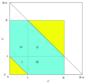
Let us rewrite for $\varepsilon\in[0,R]$ the collision integral (LABEL:eqn:qbec) as

$$Q_{R}(f)(\varepsilon)=\int_{0}^{R}\int_{S(\varepsilon,\varepsilon^{\prime})}^{D(\varepsilon,\varepsilon^{\prime})}\rho(\varepsilon_{\min})F(\varepsilon,\varepsilon^{\prime},\varepsilon^{\prime}_{*})\,d\varepsilon_{*}^{\prime}d\varepsilon^{\prime},$$ (54)

where $F(\varepsilon,\varepsilon^{\prime},\varepsilon^{\prime}_{*})=[f^{\prime}f_{*}^{\prime}(1+f)(1+f_{*})-ff_{*}(1+f^{\prime})(1+f_{*}^{\prime})]$, with $\varepsilon_{*}=\varepsilon^{\prime}+\varepsilon_{*}^{\prime}-\varepsilon$, and $S(\varepsilon,\varepsilon^{\prime})=\max\{\varepsilon-\varepsilon^{\prime},0\}$, $D(\varepsilon,\varepsilon^{\prime})=\min\{\varepsilon-\varepsilon^{\prime}+R,R\}$. The integration domain for a fixed value of $\varepsilon$ in the $(\varepsilon^{\prime},\varepsilon_{*}^{\prime})$ plane is shown in figure 1.

Figure 1: The computational domain (dark gray region) in the $(\epsilon^{\prime},\epsilon_{*}^{\prime})$ plane for a fixed $\varepsilon$

We need the following

Lemma 2.1

We have

$$\rho(\varepsilon_{\min})=\left\{\begin{array}[]{cc}\rho(\varepsilon_{*})&\quad(\varepsilon^{\prime},\varepsilon_{*}^{\prime})\in{\rm I}\\ \rho(\varepsilon)&\quad(\varepsilon^{\prime},\varepsilon_{*}^{\prime})\in{\rm II}\\ \rho(\varepsilon_{*}^{\prime})&\quad(\varepsilon^{\prime},\varepsilon_{*}^{\prime})\in{\rm III}\\ \rho(\varepsilon^{\prime})&\quad(\varepsilon^{\prime},\varepsilon_{*}^{\prime})\in{\rm IV}\end{array}\right.$$ (55)

where the regions I, II, III, IV represent a partition of the computational domain and are shown in figure 1.

Proof:

Region I is characterized by $0\leq\varepsilon_{*}^{\prime}\leq\varepsilon$ and $0\leq\varepsilon^{\prime}\leq\varepsilon$ with $\varepsilon^{\prime}+\varepsilon^{\prime}_{*}\geq\varepsilon$. Thus $\varepsilon_{*}=\varepsilon_{*}^{\prime}+\varepsilon^{\prime}-\varepsilon\leq\varepsilon$, $\varepsilon_{*}=\varepsilon_{*}^{\prime}+\varepsilon^{\prime}-\varepsilon\leq\varepsilon^{\prime}$, $\varepsilon_{*}=\varepsilon_{*}^{\prime}+\varepsilon^{\prime}-\varepsilon\leq\varepsilon_{*}^{\prime}$ and hence $\varepsilon_{\min}=\varepsilon_{*}$.

Region II is characterized by $\varepsilon^{\prime}\geq\varepsilon$ and $\varepsilon^{\prime}_{*}\geq\varepsilon$ with $\varepsilon^{\prime}+\varepsilon^{\prime}_{*}\leq R+\varepsilon$. Thus $\varepsilon_{*}=\varepsilon^{\prime}+\varepsilon^{\prime}_{*}-\varepsilon\geq\varepsilon$ and hence $\varepsilon_{\min}=\varepsilon$.

Region III is characterized by $R\geq\varepsilon^{\prime}\geq\varepsilon$ and $0\leq\varepsilon^{\prime}_{*}\leq\varepsilon$. Thus $\varepsilon_{*}=\varepsilon^{\prime}+\varepsilon^{\prime}_{*}-\varepsilon\geq\varepsilon^{\prime}_{*}$ and hence $\varepsilon_{\min}=\varepsilon^{\prime}_{*}$.

Region IV is characterized by $R\geq\varepsilon_{*}^{\prime}\geq\varepsilon$ and $0\leq\varepsilon^{\prime}\leq\varepsilon$. Thus $\varepsilon_{*}=\varepsilon^{\prime}+\varepsilon^{\prime}_{*}-\varepsilon\geq\varepsilon^{\prime}$ and hence $\varepsilon_{\min}=\varepsilon^{\prime}$.

$\square$

Using the previous lemma the integral (54) over the four regions can be decomposed as

$$Q_{R}(f)(\varepsilon)=I_{1}(\varepsilon)+I_{2}(\varepsilon)+I_{3}(\varepsilon)+I_{4}(\varepsilon),$$ (56)

with

$$I_{1}(\varepsilon) = \int_{0}^{\varepsilon}\int_{\varepsilon-\varepsilon^{\prime}}^{\varepsilon}\rho(\varepsilon^{\prime}+\varepsilon_{*}^{\prime}-\varepsilon)F(\varepsilon,\varepsilon^{\prime},\varepsilon^{\prime}_{*})\,d\varepsilon_{*}^{\prime}d\varepsilon^{\prime},$$ (57)

$$I_{2}(\varepsilon) = \int_{\varepsilon}^{R}\int_{\varepsilon}^{R+\varepsilon-\varepsilon^{\prime}}\rho(\varepsilon)F(\varepsilon,\varepsilon^{\prime},\varepsilon^{\prime}_{*})\,d\varepsilon_{*}^{\prime}d\varepsilon^{\prime},$$ (58)

$$I_{3}(\varepsilon) = \int_{\varepsilon}^{R}\int_{0}^{\varepsilon}\rho(\varepsilon_{*}^{\prime})F(\varepsilon,\varepsilon^{\prime},\varepsilon^{\prime}_{*})\,d\varepsilon_{*}^{\prime}d\varepsilon^{\prime},$$ (59)

$$I_{4}(\varepsilon) = \int_{0}^{\varepsilon}\int_{\varepsilon}^{R}\rho(\varepsilon^{\prime})F(\varepsilon,\varepsilon^{\prime},\varepsilon^{\prime}_{*})\,d\varepsilon_{*}^{\prime}d\varepsilon^{\prime}.$$ (60)

A similar decomposition holds for the quadrature formula (LABEL:eqn:qbed1)

$${\tilde{Q}}_{R}(f)(\varepsilon_{i})={\tilde{I}}_{1}(\varepsilon_{i})+{\tilde{I}}_{2}(\varepsilon_{i})+{\tilde{I}}_{3}(\varepsilon_{i})+{\tilde{I}}_{4}(\varepsilon_{i}),$$ (61)

with

$${\tilde{I}}_{1}(\varepsilon_{i}) = w^{2}\sum_{k=1}^{i}\sum_{l=i-k+1}^{i}\,\rho(\varepsilon_{k}+\varepsilon_{l}-\varepsilon_{i})F(\varepsilon_{i},\varepsilon_{k},\varepsilon_{l}),$$ (62)

$${\tilde{I}}_{2}(\varepsilon_{i}) = w^{2}\sum_{k=i+1}^{N}\sum_{l=i}^{N+i-k}\,\rho(\varepsilon_{i})F(\varepsilon_{i},\varepsilon_{k},\varepsilon_{l}),$$ (63)

$${\tilde{I}}_{3}(\varepsilon_{i}) = w^{2}\sum_{k=i+1}^{N}\sum_{l=1}^{i}\,\rho(\varepsilon_{l})F(\varepsilon_{i},\varepsilon_{k},\varepsilon_{l}),$$ (64)

$${\tilde{I}}_{4}(\varepsilon_{i}) = w^{2}\sum_{k=1}^{i}\sum_{l=i+1}^{N}\,\rho(\varepsilon_{k})F(\varepsilon_{i},\varepsilon_{k},\varepsilon_{l}).$$ (65)

From the point of view of accuracy we can state

Theorem 2.1 (Consistency)

Let the function $f$ and $\rho$ be $C^{m}([0,R])$, $m=1$ or $m=2$, then the quadrature formula (LABEL:eqn:qbed1) satisfies

$$|Q_{R}(f)(\varepsilon_{i})-{\tilde{Q}}_{R}(f)(\varepsilon_{i})|\leq R^{2}C_{m}(\Delta\varepsilon)^{m}M_{m},\qquad\Delta\varepsilon=R/N,$$ (66)

where $M_{m}$ is a constant that depends on $f$ and $\rho$ and their derivatives up to the order $m$ and if $\varepsilon_{i}=(i-1)\Delta\varepsilon$, $i=1,\ldots,N$ (rectangular rule) then $m=1$ and $C_{m}=1/2$, whereas if $\varepsilon_{i}=(i-1/2)\Delta\varepsilon$, $i=1,\ldots,N$ (midpoint rule) $m=2$ and $C_{m}=1/24$.

Proof:
First let us recall the following basic estimate for a composite product quadrature rule with equal weights (see [3] for example)

$$\left|\int_{a}^{b}\int_{c}^{d}g(x,y)dxdy-\Delta x\Delta y\sum_{i=1}^{N_{x}}\sum_{j=1}^{N_{y}}g(x_{i},y_{j})\right|\leq$$

(67)

$${(b-a)(d-c)}C_{m}\left[(\Delta x)^{m}M_{x,m}+(\Delta y)^{m}M_{y,m}\right],$$

where $\Delta x=(b-a)/N_{x}$, $\Delta y=(d-c)/N_{y}$, $M_{x,m}$ and $M_{y,m}$ are two constants such that

$$|\frac{\partial^{m}g}{\partial x^{m}}|\leq M_{x,m},\quad|\frac{\partial^{m}g}{\partial y^{m}}|\leq M_{y,m},$$

on $[a,b]\times[c,d]$ and if $x_{i}=(i-1)\Delta x$, $y_{i}=(i-1)\Delta y$ then $m=1$, $C_{m}=1/2$, whereas if $x_{i}=(i-1/2)\Delta x$, $y_{i}=(i-1/2)\Delta y$ then $m=2$, $C_{m}=1/24$.

Now, since the integrands which appear in $I_{i}$ satisfy the required regularity conditions and approximations given by ${\tilde{I}}_{i}$ are the corresponding generalized composite product quadrature rules, each error $|I_{i}-{\tilde{I}}_{i}|$ can be estimated similarly to (67). More precisely we have

$$|I_{1}(\varepsilon_{i})-{\tilde{I}}_{1}(\varepsilon_{i})| \leq {(\varepsilon_{i})^{2}}C_{m}(\Delta\varepsilon)^{m}[M^{1}_{\varepsilon^{\prime},m}(\varepsilon_{i})+M^{1}_{\varepsilon_{*}^{\prime},m}(\varepsilon_{i})],$$

$$|I_{2}(\varepsilon_{i})-{\tilde{I}}_{2}(\varepsilon_{i})| \leq {(R-\varepsilon_{i})^{2}}C_{m}(\Delta\varepsilon)^{m}[M^{2}_{\varepsilon^{\prime},m}(\varepsilon_{i})+M^{2}_{\varepsilon_{*}^{\prime},m}(\varepsilon_{i})],$$

$$|I_{3}(\varepsilon_{i})-{\tilde{I}}_{3}(\varepsilon_{i})| \leq {\varepsilon_{i}(R-\varepsilon_{i})}C_{m}(\Delta\varepsilon)^{m}[M^{3}_{\varepsilon^{\prime},m}(\varepsilon_{i})+M^{3}_{\varepsilon_{*}^{\prime},m}(\varepsilon_{i})],$$

$$|I_{4}(\varepsilon_{i})-{\tilde{I}}_{4}(\varepsilon_{i})| \leq {\varepsilon_{i}(R-\varepsilon_{i})}C_{m}(\Delta\varepsilon)^{m}[M^{4}_{\varepsilon^{\prime},m}(\varepsilon_{i})+M^{4}_{\varepsilon_{*}^{\prime},m}(\varepsilon_{i})],$$

where the constants $M^{i}_{\varepsilon^{\prime},m}(\varepsilon)$ and $M^{i}_{\varepsilon_{*}^{\prime},m}(\varepsilon)$ are suitable bounds of the partial derivatives of order $m$ of the integrand functions.

Summing up the errors we get

$$|Q_{R}(f,f)(\varepsilon_{i})-{\tilde{Q}}_{R}(\varepsilon_{i})|\leq{R^{2}}C_{m}(\Delta\varepsilon)^{m}M_{m},$$ (68)

where $M_{m}(\varepsilon)=\max_{i,k}\{M^{i}_{\varepsilon^{\prime},m}(\varepsilon_{k})+M^{i}_{\varepsilon_{*}^{\prime},m}(\varepsilon_{k})\}$.

$\square$

2.4 Fast algorithms

Finally we will analyze the problem of the computational cost of the quadrature formula (LABEL:eqn:qbed1). A straightforward analysis shows that the evaluation of the double sum in (LABEL:eqn:qbed1) at the point $\varepsilon_{i}$ requires $(2(i-1)(N-i+1)+N^{2})/2$ operations. The overall cost for all $N$ points is then approximatively $2N^{3}/3$. However using transform techniques and the decomposition (61) this $O(N^{3})$ cost can be reduced to $O(N^{2}\log_{2}N)$.

In order to do this let us set $h=k+l=i+j$ in (LABEL:eqn:qbed1) and rewrite

$${\tilde{Q}}_{R}(\varepsilon_{i}) = w^{2}\sum_{h=2}^{2N}\sum_{k=1}^{N}\,\rho(\varepsilon_{\min})[f_{k}f_{h-k}(1+f_{i})(1+f_{h-i})$$

$$- f_{i}f_{h-i}(1+f_{k})(1+f_{h-k})]\Psi_{h-i}^{[1,N]}\Psi_{h-k}^{[1,N]},$$

where we have set

$$\Psi_{i}^{[s,d]}=\left\{\begin{array}[]{cc}1&s\leq i\leq d\\ 0&{\rm otherwise}\end{array}\right.$$ (70)

In (LABEL:eqn:qbed1f) we assume that the function $f_{i}$ is extended to $i=1,\ldots,2N$ by padding zeros for $i>N$.

The sum (LABEL:eqn:qbed1f) can be split into sum over the four regions which characterize $\rho(\varepsilon_{\min})$. We shall give the details of the fast algorithm only for region I, the other regions can be treated similarly. We have

$${\tilde{I}}_{1}(\varepsilon_{i}) = w^{2}\sum_{h=2}^{2N}\sum_{k=1}^{i}\,\rho(\varepsilon_{h-i})[f_{k}f_{h-k}(1+f_{i})(1+f_{h-i})$$

$$- f_{i}f_{h-i}(1+f_{k})(1+f_{h-k})]\Psi_{h-i}^{[1,i]}\Psi_{h-k}^{[1,i]},$$

or equivalently

$${\tilde{I}}_{1}(\varepsilon_{i}) = w^{2}\sum_{h=2}^{2N}\rho(\varepsilon_{h-i})(1+f_{i})(1+f_{h-i})\Psi_{h-i}^{[1,i]}\sum_{k=1}^{i}\,f_{k}f_{h-k}\Psi_{h-k}^{[1,i]}$$

$$- w^{2}\sum_{h=2}^{2N}\rho(\varepsilon_{h-i})f_{i}f_{h-i}\Psi_{h-i}^{[1,i]}\sum_{k=1}^{i}\,(1+f_{k})(1+f_{h-k})\Psi_{h-k}^{[1,i]}$$

$$= w^{2}\sum_{h=2}^{2N}\rho(\varepsilon_{h-i})(1+f_{i})(1+f_{h-i})\Psi_{h-i}^{[1,i]}S^{1}_{h}(i)$$

$$- w^{2}\sum_{h=2}^{2N}\rho(\varepsilon_{h-i})f_{i}f_{h-i}\Psi_{h-i}^{[1,i]}S^{2}_{h}(i),$$

where we have set

$$S^{1}_{h}(i)=\sum_{k=1}^{i}\,f_{k}f_{h-k}\Psi_{h-k}^{[1,i]},\quad S^{2}_{h}(i)=\sum_{k=1}^{i}\,(1+f_{k})(1+f_{h-k})\Psi_{h-k}^{[1,i]}.$$ (72)

Now the two sums $S^{1}_{h}(i)$ and $S^{2}_{h}(i)$ are discrete convolutions and can be evaluated for all $h$ and $i$ using the FFT algorithm in $O(N^{2}\log_{2}N)$ operations. This can be easily done rewriting them in the form

$$S_{h}(i)=\sum_{k=1}^{N}\,g_{k}g_{h-k}\Psi_{h-k}^{[1,i]}\Psi_{k}^{[1,i]},$$ (73)

for a suitable choice of the discrete function $g_{i}$. It is well known that for $N=2^{\alpha}$ with $\alpha$ integer the sum (73) can be computed for each $i$ via FFT in $O(N\log_{2}N))=O(2^{\alpha}\alpha)$ operations. The total cost to compute $S_{h}(i)$ for all $i$ is then $O(N^{2}\log_{2}N)$.

A better algorithm can be obtained if we rewrite the sums $S^{1}_{h}(i)$ and $S^{2}_{h}(i)$ in the form

$$S_{h}(i)=\sum_{k=1}^{2^{\beta_{i}}}\,g_{k}g_{h-k}\Psi_{h-k}^{[1,i]}\Psi_{k}^{[1,i]},$$ (74)

where

$$\beta_{i}=\left\{\begin{array}[]{cc}[[\log_{2}(i-1)]]+1&\quad i>1\\ 0&\quad i=1\end{array}\right.$$ (75)

and $[[\cdot]]$ denotes the integer part.

For each $i$ the convolution sum (74) now can be computed in $O(2^{\beta_{i}}\beta_{i})$ operations. The total cost will be approximatively reduced by one half since $O(\sum_{i=1}^{N}i\log_{2}i)\approx O(\frac{1}{2}N^{2}\log_{2}(N))$.

Clearly once expressions $S^{1}_{h}(i)$ and $S^{2}_{h}(i)$ have been computed the remaining two sums are of the type

$$g_{i}\sum_{h=2}^{2N}g_{h-i}\Psi_{h-i}^{[1,i]}S_{h}(i),$$ (76)

which can be computed directly with $O(N^{2})$ operations. Thus the final cost for the computation of ${\tilde{I}}_{1}(\varepsilon_{i})$ for all $i$ is $O(N^{2}\log_{2}N+N^{2})=O(N^{2}\log_{2}N)$.

Remark 3

In the case of constant $\rho$ it is easy to show that expression (LABEL:eqn:qbed1f) reduces to a double convolution sum which can be evaluated using the FFT in only $O(N\log_{2}N)$ operations instead of $O(N^{2}\log_{2}N)$.

Figure 2: The relative $L_{1}$ error for scheme QBF1 (left) and QBF2 (right) computed with $N=20$ (solid line), $N=40$ (dotted line), $N=80$ (dash-dot line) points for $t\in[0,2.5]$.

Figure 3: Convergence rates for scheme QBF1 (left) and QBF2 (right) computed with $N=20,40$ (solid line), $N=40,80$ (dotted line) points for $t\in[0,2.5]$.

3 Numerical tests and applications

In this section we test the performance of the proposed schemes by considering their behavior in different physical and mathematical situations. We shall refer to the first and second order fast schemes developed in the previous section by QBF1 and QBF2 respectively. The time integration is performed with standard first and second order explicit Runge-Kutta schemes after dividing equation (45) by $\rho(\varepsilon_{i})$ and thus rewriting the semidiscrete schemes as

$$\frac{\partial f_{i}}{\partial t} = w^{2}\sum_{{j,l=1}\atop{1\leq k=i+j-l\leq N}}^{N}\,\frac{\rho(\varepsilon_{\min})}{\rho(\varepsilon_{i})}[f_{k}f_{l}(1+f_{i})(1+f_{j})$$

$$- f_{i}f_{j}(1+f_{k})(1+f_{l})].$$

In all our numerical tests the density of states is given by

$$\rho(\varepsilon)=\frac{\varepsilon^{2}}{2},$$ (78)

which corresponds to an harmonic potential $V(x)$.

Note that $0\leq{\rho(\varepsilon_{\min})}/{\rho(\varepsilon_{i})}\leq 1$ for $\varepsilon_{i}\neq 0$ and that as $\varepsilon_{i}\to 0$ we have ${\rho(\varepsilon_{\min})}/{\rho(\varepsilon_{i})}\to 1$. Furthermore since $\rho(0)=0$ the values of the distribution function at $\varepsilon_{i}=0$ does not affect the discrete conservation of mass and energy.

The schemes were implemented using the fast algorithm described in Section 2.4.

3.1 Accuracy analysis

The first test case has been used to check the numerical convergence of our quadrature formulas by neglecting the time discretization error (as usual this can be achieved either using very small time steps or sufficiently accurate time discretizations). The initial datum is a Gaussian profile centered at $R/2$

$$f=\exp(-4(\varepsilon-R/2)^{2}),$$ (79)

with $R=10$. The final integration time is $T=2.5$. We report in Figure 2 the relative errors in the $L_{1}-$norm obtained with the different schemes for $N=20,40,80$ grid points. As a reference solution we used the numerical result obtained with a fine grid of $N=160$ points.

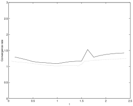
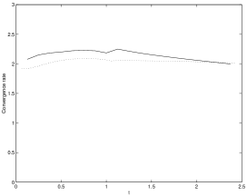
In Figure 3 the corresponding convergence rates of the schemes are reported. As usual given two error curves $E_{N}$ and $E_{2N}$ corresponding to $N$ and $2N$ grid points the convergence rate is computed as

$$\log_{2}\left(\frac{E_{N}}{E_{2N}}\right).$$

The results confirm the expected first order and second order degree of accuracy of the methods.

Remark 4

Since the midpoint rule, similarly to the trapezoidal rule, admits an Euler-MacLaurin expansion we can in principle increase the order of the method by extrapolation techniques. Unfortunately with this approach it is difficult to keep conservations as well as entropy inequality.

3.2 Bose-Einstein equilibrium

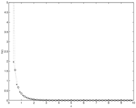
Next we consider the same initial data as in the previous section and compute the large time behavior of the schemes for $N=40$. The stationary solution at $t=10$ is given in Figure 4 for both schemes together with the numerically computed entropy growth. As observed the methods converge to the same stationary state given by a ’regular’ discrete Bose-Einstein distribution.

Figure 4: Stationary discrete Bose-Einstein equilibrium and entropy growth for scheme QBF1 ($\circ$) and QBF2 ($\times$) computed with $N=40$ points.

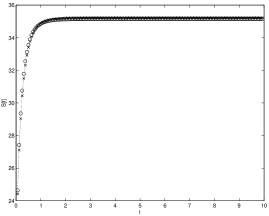
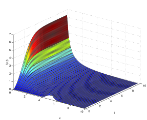
The trend to equilibrium in time for the two schemes is reported in Figures 5. Note that although the two schemes agree very well there is a remarkable resolution difference in proximity of the point $\varepsilon=0$ due to the staggered grids of the schemes.

Figure 5: Trend to equilibrium in time for scheme QBF1 (left) and QBF2 (right) computed with $N=40$ points.

However since the value of $f$ at $\varepsilon=0$ does not affect the macroscopic quantities and the entropy we can adopt a suitable extrapolation strategy to recover a better resolution of scheme QBF2 near $\varepsilon=0$. Since we are mostly interested in the large time behavior of the solution we can recover the value at the zero energy level by a steady state extrapolation. This corresponds to assume $f$ of the form (53) and consequently to assign

$$f(0)=\frac{1}{e^{\beta}-1},\quad\beta=\log\left(\frac{f_{2}+1}{f_{2}}\right)+\frac{1}{\Delta\varepsilon}\log\left(\frac{f_{2}(f_{2}+1)}{f_{1}(f_{1}+1)}\right).$$ (80)

In Table 1 we compare the extrapolated results at the final computation time of scheme QBF2 for different extrapolation methods with scheme QBF1 and with the “exact” steady state solution. We remark that the values of $\alpha$ and $\beta$ for the stationary state can be computed by inverting numerically the equations (29)-(30) for $f_{\infty}$ given by (28). The marked improvement in the resolution given by scheme QBF2 with steady state extrapolation is evident.

Exact	QBF1	QBF2 with extrapolation
		Steady state	Exponential	Cubic	Linear
7.144	6.335	7.217	6.449	6.323	5.994

Table 1: Values of $f(0)$ at $t=10$ with $N=40$ points.

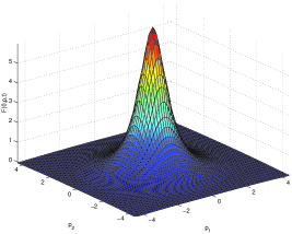
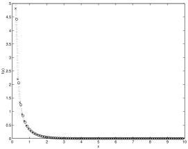
In Figure 6 we present the corresponding result for scheme QBF2 with steady state extrapolation at $\varepsilon=0$ (as we shall always do from now on with QBF2). In the same figure we also report the final “steady” solution at $t=10$ for the phase-space density reconstructed at $x=0$ and $p=(p_{1},p_{2},0)$.

Figure 6: Trend to equilibrium in time for scheme QBF2 (left) and stationary phase-space density reconstructed at $x=0$ and $p=(p_{1},p_{2},0)$ (right) with steady state extrapolation at $\varepsilon=0$.

3.3 Condensation

In this test we consider the process of condensation of bosons. It is a fundamental results of quantum statistics of bosons that above a critical density/below a critical energy particles enter the ground state, i.e. a Bose-Einstein condensate forms (see [19],[20],[18],[16],[17]) and the equilibrium distribution $f_{\infty}$ is of the form (31) with $\beta_{-}\neq 0$.

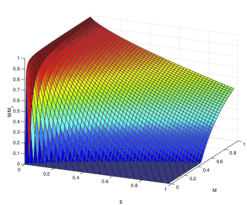
In general the evaluation of the condensate fraction as a function of time is a challenging problem from the computational viewpoint. If we assume the density function $f$ to be of the form (31), which corresponds to the long time behavior, we can use the following method to identify if condensation will occur and compute the equilibrium condensate mass for a given mass energy pair $(M,E)$.

First solve numerically for $\alpha$ the equation

$$E=\int_{0}^{\infty}\frac{\rho(\varepsilon)\varepsilon}{\exp(\alpha\varepsilon)-1}\,d\varepsilon.$$ (81)

Then compute

$$I_{\alpha}=\int_{0}^{\infty}\frac{\rho(\varepsilon)}{\exp(\alpha\varepsilon)-1}\,d\varepsilon.$$ (82)

If $I(\alpha)<M$ the mass entropy pair is critical and condensation will take place. The condensate mass fraction in equilibrium can then be computed

$$\frac{M_{c}}{M}=1-\frac{I_{\alpha}}{M}.$$ (83)

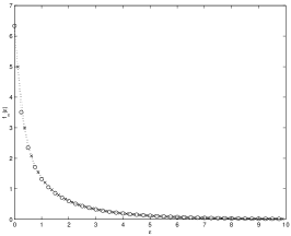
We report in Figure 7 the condensate mass fraction computed with the previous method for $(M,E)\in[0,1]\times[0,1]$.

Figure 7: Mass fraction of the condensate in the mass-energy plane at the stationary state.

A related challenging problem is the computation of the critical time at which the condensate starts to form. In order to do this we consider two different numerical indicators.

We recall that for the second order method, unlike the first order one, due to the midpoint quadrature, we have $\varepsilon_{i}\neq 0$ for all gridpoints. This makes scheme QBF2 more suitable to treat situations where the solution is close to be singular at $\varepsilon=0$. In particular, in such cases, it is impossible to extrapolate the value $f(0)$ with a positive $\beta$. Thus whenever steady state extrapolation is impossible we can assume to have formation of condensate at $\varepsilon=0$.

For the scheme QBF1 we expect the value of $f(0)$ to increase dramatically when formation of condensate takes place. In this case we can use as an indicator of the formation of condensate the expression [13]

$$C_{F}=\frac{\Delta\varepsilon f_{0}}{\Delta\varepsilon\sum_{i}f_{i}}.$$ (84)

For the numerical test we choose the initial distribution in the energy interval $[0,R]$ with $R=10$ to be[16],[17]

$$f(\epsilon)=\frac{2\bar{f}}{\pi}\arctan(e^{\Gamma(1-\epsilon/\epsilon_{0})}),$$ (85)

with $\Gamma=5$ and $\epsilon_{0}=R/8$. At values of $\bar{f}$ larger than a critical $\bar{f}^{*}$ the formation of a condensate occurs (see [16],[17] for similar results in the homogeneous case). We choose $\bar{f}=1$, which turns on to be supercritical. In this case the mass energy pair is approximatively $(0.42,0.50)$ which corresponds to a condensate mass fraction of $\approx 0.3$ at the stationary state (see Figure 7). Using $N=320$ points and scheme QBF2 with steady state extrapolation the condensate formation in finite time at $t_{c}\approx 4.2$ is observed.

Figure 8: Estimation of the critical time using the numerical indicator $C_{F}$ in time for $N=80,160,320$ for scheme QBF1 (left) and scheme QBF2 with steady state extrapolation (right).

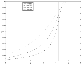
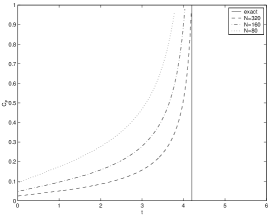
We report in Figure 8 the time evolution of the indicator (84) for scheme QBF1 and for scheme QBF2 with steady state extrapolation before the critical time. The vertical line correspond to the critical time at which the steady state extrapolation fails. The results indicate the numerical convergence of the approximation (84).

Figure 9: Distribution of bosons at different times in logarithmic scale before the critical time for scheme QBF1 (left) and scheme QBF2 with steady state extrapolation (right) for $N=320$.

Figure 10: Magnified view of the distribution of bosons after the critical time of condensation with scheme QBF1 ($\circ$) and scheme QBF2 ($\times$) with $N=40$ (left) and $N=80$ (right) points at time $t=15$.

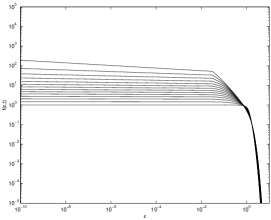
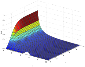
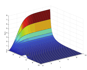
The distribution of bosons at different times in logarithmic scale before the critical time is shown in Figure 9 for scheme QBF1 (left) and scheme QBF2 with steady state extrapolation (right) .

A magnified view of the numerical solutions obtained with $N=40$ and $N=80$ points at $t=15$ shows that away from the singularity the two schemes are still in good agreement (see Figure 10).

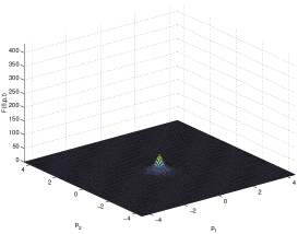
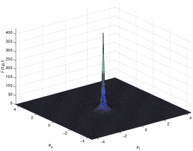
Finally in Figure 11 we also report the phase-space density reconstructed at $x=0$ and $p=(p_{1},p_{2},0)$ at two different times before the critical time. The corresponding solution has been obtained for $N=80$ with scheme QBF2 and steady state extrapolation.

Figure 11: Phase-space density reconstructed at $x=0$ and $p=(p_{1},p_{2},0)$ for scheme QBF2 with steady state extrapolation at $\varepsilon=0$ at $t=3.4$ (left) and $t=3.75$ (right).

4 Conclusions

We have developed first and second order fast solvers for the Boson Boltzmann equation assuming a boson distribution which only depends on the total energy. The methods preserve all the relevant physical properties (conservation of mass and energy, entropy inequality and steady states). The performance of the schemes has been tested for both Bose-Einstein and generalized Bose-Einstein steady states. The numerical methods have shown the capability to describe well the challenging phenomenon of condensation of bosons.

We remark that, to our knowledge, this is the first example of accurate, conservative and fast deterministic numerical method for a Boltzmann equation. Previous results were available in the literature for Fokker-Planck-Landau type equations (see [2],[8],[14]) or using some suitable approximations of the Boltzmann equation (see the recent review [12] and the references therein).

Note that the present numerical methods can be applied directly even to the case of the energy dependent quantum Boltzmann equation for Fermions as well as the classical Boltzmann equation of rarefied gas dynamics.

We hope to extend in the future these ideas to time dependent potentials [13].

Acknowledgement

The authors are grateful to Dieter Jaksch for stimulating discussions and physical explanations on the subject of this work. We also thank the anonymous referee for constructive suggestions.

References

- [1] S.N. Bose, Plancks Gesetz and Lichtquantenhypothese, Z. Phys., 26, 178–181, (1924).
- [2] C. Buet, S. Cordier, P. Degond and M. Lemou, Fast algorithms for numerical, conservative, and entropy approximations of the Fokker-Planck equation, J. Comp. Phys., 133, 310-322, (1997).
- [3] P.J.Davis, P.Rabinowitz, Methods of numerical integration, Academic Press, (1975).
- [4] A.Einstein, Quantentheorie des einatomingen idealen gases, Stiz. Presussische Akademie der Wissenshaften Phys-math. Klasse, Sitzungsberichte, 23, 1–14, (1925).
- [5] A.Einstein, Zur quantentheorie des idealen gases, Stiz. Presussische Akademie der Wissenshaften Phys-math. Klasse, Sitzungsberichte, 23, 18–25, (1925).
- [6] M.Escobedo, S.Mischler, M.A.Valle, Homogeneous Boltzmann equation for quantum and relativistic particles, Electron. J. Diff. Eqns., Monograph 04 (2003), 85 pages.
- [7] M.Escobedo, S.Mischler, On a quantum Boltzmann equation for a gas of photons, J. Math. Pures Appl., 9 80, 471–515, (2001).
- [8] M.Lemou, Multipole expansions for the Fokker-Planck-Landau operator, Numerische Mathematik, 78, 597–618, (1998).
- [9] O.J.Luiten, M.W.Reynolds, J.T.M.Walraven, Kinetic theory of evaporative cooling, Phys. Rev. A, 53, 381–389, (1996).
- [10] X.Lu, On spatially homogeneous solutions of a modified Boltzmann equation for Fermi-Dirac particles, J. Statist. Phys., 105, 353–388, (2001).
- [11] X.Lu, A modified Boltzmann equation for Bose-Einstein particles: isotropic solutions and long-time behavior, J. Statist. Phys., 98, 1335–1394, (2000).
- [12] L. Pareschi, Computational methods and fast algorithms for Boltzmann equations, Lecture Notes on the discretization of the Boltzmann equation, Chapter 7, Series on Advances in Mathematics for Applied Sciences, Vol. 63, World Scientific, (2003).
- [13] L.Pareschi, D.Jaksch, P.Markowich, M.Wenin, P.Zoller, Increasing phase-space density by varying the trap potential in Bose-Einstein condensation, preprint (2004).
- [14] L. Pareschi, G. Russo and G. Toscani, Fast spectral methods for the Fokker-Planck-Landau collision operator, J. Comp. Phys, 165, 1–21, (2000).
- [15] L. Pareschi, G.Toscani and C. Villani, Spectral methods for the non cut-off Boltzmann equation and numerical grazing collision limit, Numerische Mathematik, 93, pp.527-548, (2003).
- [16] D.V.Semikoz, I.I.Tkachev, Kinetics of Bose condensation, Physical Review Letters, 74, 3093–3097, (1995).
- [17] D.V.Semikoz, I.I.Tkachev, Condensation of bosons in the kinetic regime, Physical Review D, 55, 489–502, (1997).
- [18] C.W.Gardiner, D.Jaksch, P.Zoller, Quantum kinetic theory II, Phys. Rev. A, 56, 575, (1997)
- [19] C.W.Gardiner, P.Zoller, Quantum kinetic theory, Phys. Rev. A, 55, 2902, (1997),
- [20] C.W.Gardiner, P.Zoller, Quantum kinetic theory III, Phys. Rev. A, 58, 536, (1998)