Weak Lensing Peak Finding: Estimators, Filters, and Biases

Abstract

Large catalogs of shear-selected peaks have recently become a reality. In order to properly interpret the abundance and properties of these peaks, it is necessary to take into account the effects of the clustering of source galaxies, among themselves and with the lens. In addition, the preferred selection of lensed galaxies in a flux- and size-limited sample leads to fluctuations in the apparent source density which correlate with the lensing field (lensing bias). In this paper, we investigate these issues for two different choices of shear estimators which are commonly in use today: globally-normalized and locally-normalized estimators. While in principle equivalent, in practice these estimators respond differently to systematic effects such as lensing bias and cluster member dilution. Furthermore, we find that which estimator is statistically superior depends on the specific shape of the filter employed for peak finding; suboptimal choices of the estimator+filter combination can result in a suppression of the number of high peaks by orders of magnitude. Lensing bias generally acts to increase the signal-to-noise $\nu$ of shear peaks; for high peaks the boost can be as large as $\Delta\nu\approx 1-2$. Due to the steepness of the peak abundance function, these boosts can result in a significant increase in the abundance of shear peaks. A companion paper (Rozo et al., 2010a) investigates these same issues within the context of stacked weak lensing mass estimates.

1. Introduction

The abundance of rare massive objects (clusters) in the Universe has emerged as a powerful probe of cosmology (Vikhlinin et al., 2009; Rozo et al., 2010b; Mantz et al., 2009; Henry et al., 2009; Vanderlinde et al., 2010). Many different techniques can be used to find these clusters, such as optical identification, X-rays, Sunyaev-Zeldovich effect, and gravitational lensing. Among these, lensing stands out as being the least sensitive to the complicated baryonic physics that govern galaxy formation and the non-thermal processes that affect the dynamics of the intra-cluster medium. Consequently, the lensing signal is expected to be the easiest to predict, a fact that has fostered great interest in developing weak lensing cluster finders (Schneider, 1996; Hennawi and Spergel, 2005; Hamana et al., 2004), and has even lead to the publication of several lensing selected cluster samples (Miyazaki et al., 2007; Wittman et al., 2006; Gavazzi and Soucail, 2007). In practice, lensing selection suffers from significant projection effects: the lensing signal of a cluster can be enhanced by a favorable projection of a triaxial halo; by associated mass distributions (substructure filaments); or by the chance superposition of large-scale structure along the line of sight. Fortunately, such superpositions can be calibrated by relying on numerical simulations, and weak lensing peak statistics remain a promising probe for cosmological physics (Wang et al., 2009; Dietrich and Hartlap, 2009; Kratochvil et al., 2009; Marian et al., 2010).

Weak lensing shear measurements use the shapes of distant galaxies in order to statistically extract the lensing signal. To date, most work has assumed that source galaxies are randomly distributed, whereas in practice we know galaxies are clustered. The apparent clustering receives two contributions: one from intrinsic (physical) clustering of the galaxies, henceforth referred to as source clustering; the other from fluctuations in the galaxy density induced by lensing itself, via lensing bias (also known as magnification bias; Broadhurst et al., 1995; Schmidt et al., 2009a). The intrinsic clustering of source galaxies acts to increase the noise in the shear measurement, while the lensing-induced fluctuations can bias the shear measurement if they are not properly accounted for. In fact, lensing bias can be seen as a probe of weak gravitational lensing in its own right (Schneider et al., 2000; Van Waerbeke et al., 2010, Rozo and Schmidt, in preparation).

In a companion paper (Rozo et al., 2010a, henceforth referred to as paper I), we study similar issues for stacked weak lensing analyses of groups and clusters. The two papers are highly complementary, as paper I focuses on high signal-to-noise weak lensing mass calibration of objects that have been previously identified and then stacked, whereas in this work we focus on identifying shear peaks in the low signal-to-noise regime.

Following paper I, we discuss two possible filtered shear estimators, which differ in the way the estimator is normalized. The first estimator uses a fixed normalization (e.g., Maturi et al. (2005); Wang et al. (2009)), and is therefore sensitive to the overall modulation of the source density field by the lensing signal. The second estimator uses an individual normalization for each point in the sky (e.g., Miyazaki et al. (2007)). In this approach, the fluctuations in the density of background galaxies are partially canceled out, which reduces noise, but also shrinks the extra signal due to magnification. Moreover, a location-based normalization estimator can lead to dilution of the lensing signal if the source population is contaminated by cluster galaxies (see paper I for a more detailed discussion).

Throughout, we adopt a fiducial flat $\Lambda$CDM cosmology with $h=0.7$, $\Omega_{m}=0.28$, $n_{s}=0.96$, and a power spectrum normalization of $\sigma_{8}=0.85$ at $z=0$. All masses are defined as $M_{200m}$, i.e. enclosing an average density of 200 times the mean matter density. The source galaxies are assumed to follow the redshift distribution expected for the Dark Energy Survey (DES),

$$\frac{dN}{dz}\propto z^{2}\exp\left[-(z/z_{0})^{\beta}\right]$$ (1)

with $z_{0}=0.5$ and $\beta=1.4$, and we assumed a density of $\bar{n}=20$ arcmin^-2. This source density is slightly larger than that expected for DES, but smaller than that of other future surveys such as Hyper Suprime-Cam or the Large Synoptic Survey Telescope (LSST).

Section 2 presents the shear estimators, and discusses how lensing bias impacts each of these estimators in turn. We also discuss the choice of filter function and optimal filter scale. Section 3 presents the results on the statistics of lensing peaks. We conclude in Section 4. Details on the lensing calculations, and two derivations regarding the variance of smoothed shear filters have been relegated to the appendix.

2. Smoothed Shear Estimators

In this section, we focus on estimators of the form

$$\hat{A}(\vec{\theta})=\frac{1}{\bar{n}}\sum_{i}e_{i}W(\vec{\theta}_{i}-\vec{\theta}).$$ (2)

where the sum is over all galaxies, $\bar{n}$ is the mean source galaxy density, $e_{i}$ is the tangential component of the ellipticity of galaxy $i$ (with respect to the relative position $\vec{\theta}_{i}-\vec{\theta}$), and $W$ is an arbitrary filter which we assume is unity-normalized,

$$\int d^{2}\theta\>W(\vec{\theta})=1.$$ (3)

For the time being, we leave the filter unspecified. The estimator Eq. (2) has a fixed normalization. We consider the alternative choice of a varying normalization in Section 2.3.

In order to derive the statistical properties of $\hat{A}$, we proceed as follows: first, we divide the sky into infinitesimal pixels of area $\Delta\Omega$ such that the number of galaxies in each pixel is either $0$ or $1$. Letting $n(\vec{\theta})$ be the galaxy density field on the sky, we can rewrite Eq. (2) as

$$\hat{A}(\vec{\theta})=\frac{1}{\bar{n}}\sum_{i}n_{i}e_{i}W_{i}\Delta\Omega.$$ (4)

where the sum is now over all pixels, and the index $i$ denotes that the quantity of interest is evaluated at $\vec{\theta}_{i}$. For example, $n_{i}=n(\vec{\theta}_{i})$. We now set

$$n_{i}=\bar{n}(1+\delta_{i})$$ (5)

where $\delta_{i}$ is the galaxy density fluctuation (in this section, we assume the fluctuations are purely Poisson). Assuming $\langle e_{i}\rangle=g_{i}$ where $g=\gamma/(1-\kappa)$ is the reduced (tangential) shear, we find that the expectation value of $\hat{A}$ is given by

$$\langle\hat{A}(\vec{\theta})\rangle=\sum_{i}g_{i}W_{i}\Delta\Omega=\int d^{2}\theta^{\prime}g(\vec{\theta}^{\prime})W(|\vec{\theta}-\vec{\theta}^{\prime}|).$$ (6)

For the second equality, we have let $\Delta\Omega\rightarrow 0$ (continuum limit), and correspondingly replaced $\sum_{i}\Delta\Omega$ with $\int d^{2}\theta$. Further, we have assumed that the source galaxy overdensity $\delta$ is uncorrelated with the shear. In the following discussion, we will set $\vec{\theta}=0$ without loss of generality. We can compute the variance of $\hat{A}$ in a similar fashion. In particular, using Eq. (4) and Eq. (5) we find

$$\hat{A}^{2}=\sum_{ij}(1+\delta_{i}\delta_{j})e_{i}e_{j}W_{i}W_{j}(\Delta\Omega)^{2}$$ (7)

where have ignored terms proportional to $\delta$ since these will go to zero upon taking the expectation value. Neglecting any clustering of the source galaxies for the moment, we have

$$\langle\delta_{i}\delta_{j}\rangle=\frac{1}{\bar{n}\Delta\Omega}\delta_{ij},$$ (8)

while the expectation value of the galaxy ellipticities takes the form (recall that $e_{i}$ stands for the tangential component of the ellipticity)

$$\langle e_{i}e_{j}\rangle=g_{i}g_{j}+\frac{\sigma_{e}^{2}}{2}\delta_{ij}.$$ (9)

Here, $\sigma_{e}$ denotes the RMS (intrinsic) galaxy ellipticity of the sample. Using these expressions, taking the expectation value of Eq. (7), and subtracting off $\langle\hat{A}\rangle^{2}$, we find

$${\rm Var}(\hat{A})=\frac{1}{\bar{n}}\int d^{2}\theta\ W^{2}(\vec{\theta})\left(\frac{\sigma_{e}^{2}}{2}+g^{2}(\vec{\theta})\right).$$ (10)

In many cases, $|g|\ll\sigma_{e}\sim 0.3$ and the term $g^{2}(\vec{\theta})$ in Eq. (10) is often neglected. In that case,

$${\rm Var}(\hat{A})=\frac{\sigma_{e}^{2}}{2\bar{n}}\int d^{2}\theta\>W^{2}(\vec{\theta})=\frac{\sigma_{e}^{2}}{2\bar{n}}\frac{1}{4\pi\Theta^{2}},$$ (11)

where for the second equality we have assumed a Gaussian shear filter of width $\Theta$ [Eq. (12)], which is the standard result for the variance of $\hat{A}$ (van Waerbeke, 2000).

2.1. Filter Functions

A variety of smoothing kernels have been proposed for averaging the shear, including top-hat, aperture mass (Schneider et al. (1997)), and matched filters (Maturi et al. (2005); Marian and Bernstein (2006)). Some differences in the filters are due to the various goals they were designed to achieve; for example, to reduce contributions from small scales, or large scales, or the mass-sheet degeneracy present in shear measurements.

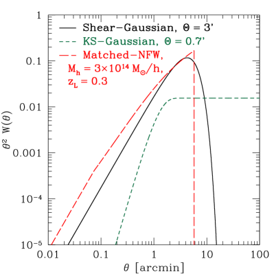
Figure 1.— Shear filter functions considered in this paper, as a function of angular separation: Gaussian-smoothed shear filter; Gaussian-smoothed convergence filter using the method of Kaiser and Squires (1993); and matched NFW filter (Marian and Bernstein, 2006).

In this paper, we will discuss three commonly used or proposed filters, which are shown in Fig. 1. It is instructive to compare this figure with Fig. 8 in the appendix, which shows the angular scales contributing to the lensing signal. Our first and perhaps simplest choice is a Gaussian shear filter,

$$W(\theta)=\frac{1}{2\pi\>\Theta^{2}}\exp\left(-\frac{\theta^{2}}{2\Theta^{2}}\right),$$ (12)

where $\Theta$ denotes the filter scale, which can be chosen to maximize signal-to-noise for a given lens mass and redshift. This filter is also similar in shape to the filter presented in Maturi et al. (2005) designed to reduce the contribution from unassociated large-scale structure.

Another choice is a filter constructed using the method of Kaiser and Squires (1993) to yield an estimator of the Gaussian-smoothed convergence $\kappa$ (“KS-Gaussian”). This is equivalent to searching for peaks in smoothed convergence maps (e.g., Hamana et al., 2004; Wang et al., 2009, but see caveats below). The shear filter function is given by:

$$W(\theta)=\frac{1}{\pi\theta^{2}}\left[1-\left(1+\frac{\theta^{2}}{2\Theta^{2}}\right)\exp\left(-\frac{\theta^{2}}{2\Theta^{2}}\right)\right],$$ (13)

where $\Theta$ is the width of the Gaussian convergence filter. This filter is usually used by pixelizing the sky in patches of a few arcmin² area, and measuring the average shear in each pixel. The resulting shear map is then convolved with the KS-Gaussian filter. While we do not explicitly consider pixelized estimators here, under certain conditions the globally-normalized estimator Eq. (2) is equivalent to a pixelized estimator: this is the case if either the shear in each pixel is estimated with a global normalization (such as in Eq. (2)), and pixels are weighted equally; or if the shear in a pixel is measured with a local normalization, and each pixel is then inverse-variance weighted, i.e. weighted by the number of galaxies in the pixel, in the further analysis.

Note that this filter is not normalizable through Eq. (3). Instead, the normalization is defined through the convergence filter. Due to the non-local relationship between shear and convergence, this filter is quite different from the Gaussian shear filter. As shown in Fig. 1, small scales are downweighted, while in principle arbitrarily large scale scales are weighted equally ($\theta^{2}\,W\sim$ const). This is a consequence of the mass-sheet degeneracy present in the shear, which can only be broken by including very large scales. We will see that due to these differences, a shear estimator using the KS-Gaussian filter behaves quite differently than an estimator using the other filters discussed here.

Finally, one can choose a filter matched to the expected signal of a Navarro-Frenk-White (NFW, Navarro et al. (1996)) lensing halo. Following Marian and Bernstein (2006), we choose

$$W(\theta)=C\>g(\theta),$$ (14)

where $g$ is the reduced shear profile of an NFW halo (see Appendix A), and the constant is determined from the normalization constraint Eq. (3). Note that as written, the filter is optimal for uniform noise and in the absence of lensing bias; it can easily be generalized to take into account the effects discussed in this paper. In Marian and Bernstein (2006), the filter was truncated at the scale corresponding to the virial radius (or $R_{200}$) of the halo (i.e. $W=0$ for $\theta>\theta_{\rm max}$); in general, one can vary the truncation scale of the filter. Fig. 1 shows that the matched-NFW filter (with truncation at $R_{200}$) is in fact quite similar to the Gaussian shear filter.

We will return to the choice of filter and optimal filter scale $\Theta$ in Section 2.5.

2.2. Lensing bias and Source Clustering

In the presence of foreground lensing matter, the number density of a flux- and size-limited sample of background galaxies is affected by two effects: galaxies get pushed over the flux and/or size threshold by lensing magnification, and their density is diluted because the observed patch of sky is stretched (Broadhurst et al. (1995)). These two effects combine in such a way that the observed source galaxy density field is related to the unlensed background density field via

$$n_{\rm obs}(\vec{\theta})=\bar{n}[1+\delta_{g}(\vec{\theta})]\mu(\vec{\theta})^{q/2}$$ (15)

where the magnification $\mu$ is given by

$$\mu(\vec{\theta})=\frac{1}{(1-\kappa)^{2}-|\gamma|^{2}}=1+2\kappa+3\kappa^{2}+|\gamma|^{2}+\dots,$$ (16)

and $q$ characterizes the contributions from magnification and size bias (Schmidt et al. (2009a, b)). Specifically, the parameter $q$ is given in terms of $\beta_{f}$ and $\beta_{r}$, the logarithmic slopes of the flux and size distributions, as:

$$q=2\beta_{f}+ \beta_{r}-2$$ (17)

$$\beta_{f}\equiv-\frac{d\ln n_{\rm obs}}{d\ln f}\Big{|}_{f=f_{\rm min}},\quad \beta_{r}\equiv-\frac{d\ln n_{\rm obs}}{d\ln r}\Big{|}_{r=r_{\rm min}}.$$ (18)

Here $f$ denotes flux and $r$ stands for apparent size of the galaxies. For definiteness, we assume a value of $q=1.5$, in the middle of the range estimated by Schmidt et al. (2009a). Consider now the expectation value of $\hat{A}$ in the presence of lensing bias. Inserting Eq. (15) into Eq. (4) and taking the expectation value we find

$$\langle\hat{A}\rangle=\int d^{2}\theta\ \mu^{q/2}(\vec{\theta})g(\vec{\theta})W(\vec{\theta})\\$$ (19)

where we have assumed the lensing field does not correlated with the source density field $\delta_{g}$. We see that the increase in the number of background sources (assuming $q>0$) leads to a higher signal, as expected.

We turn now to estimating the variance of $\hat{A}$ in the presence of magnification bias and source clustering. We assume that a weak lensing shear peak occurs when $\hat{A}$ is evaluated at the center of a lensing halo. For now, we assume that there is no contribution to the lensing shear and magnification from other matter along the line of sight. The clustering of the source population which we neglected in Section 2 is an additional noise contribution to $\hat{A}$. Using Eq. (15), we have

$$\langle\delta_{i}\delta_{j}\rangle=\frac{1}{\bar{n}\>\mu^{q/2}\Delta\Omega}\delta_{ij}+\xi_{ij}$$ (20)

where $\xi_{ij}=\xi(|\vec{\theta}_{i}-\vec{\theta}_{j}|)$ is the source galaxy angular correlation function. Here, we neglect higher moments of the angular distribution of source galaxies, which can become relevant on very small scales. In order to calculate $\xi$, we make another approximation: we assume that galaxies follow the matter distribution with a linear bias of $\sim 1$, and use the fitting formula of Smith et al. (2003) for the non-linear matter power spectrum together with the redshift distribution Eq. (1) (see also appendix of paper I). Note that $\xi$ is the observed correlation function, which in principle is also modified by lensing bias induced by large-scale structure (Matsubara, 2000; Hui et al., 2007). Since this is a small ($<10$%) correction to a usually subdominant noise contribution, we neglect this lensing bias here given our rough approximations for $\xi$. However, we do take into account that magnification modifies the source density through lensing bias, and correspondingly affects the shot noise.

The mean and variance of source ellipticities remain unchanged by lensing bias, so that as before $\langle e_{i}\rangle=g_{i}$ and $\langle e_{i}e_{j}\rangle=\frac{\sigma_{e}^{2}}{2}\delta_{ij}+g_{i}g_{j}$.

Putting everything together and plugging into Eq. (7) we find

$${\rm Var}(\hat{A}) = V_{\rm shot}+V_{\rm src}$$ (21)

$$V_{\rm shot} = \frac{1}{\bar{n}}\int d^{2}\theta\ \mu^{q/2}(\vec{\theta})W^{2}(\vec{\theta})\left(\frac{\sigma_{e}^{2}}{2}+g^{2}(\vec{\theta})\right)\ \$$ (22)

$$V_{\rm src} = \int d^{2}\theta\int d^{2}\theta^{\prime}\ S\>S^{\prime}\>\xi(|\vec{\theta}-\vec{\theta}^{\prime}|),$$ (23)

where

$$S(\vec{\theta})=\mu^{q/2}(\vec{\theta})g(\vec{\theta})W(\vec{\theta}),$$ (24)

and primed and un-primed variables are evaluated at $\vec{\theta}^{\prime}$ and $\vec{\theta}$ respectively. We have split the variance of $\hat{A}$ into a shot-noise contribution $V_{\rm shot}$, and a contribution from source clustering $V_{\rm src}$. Comparing Eq. (21) with Eq. (10) we see that lensing bias increases the shot noise in $\hat{A}$ due to the increased source density (but not as fast as it increases the value of $\hat{A}$ itself). In addition, the clustering of source galaxies adds to the variance of $\hat{A}$.

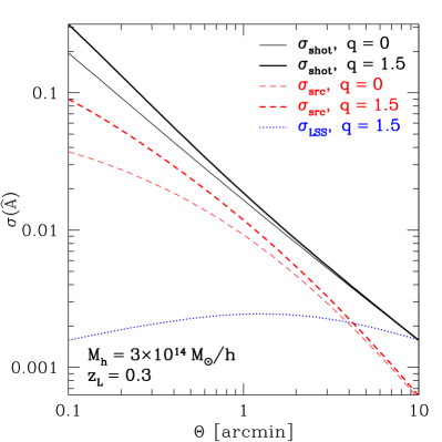
Figure 2.— Contributions to the variance of smoothed shear estimators as a function of filter scale $\Theta$ for a Gaussian shear filter: shot noise $\sigma_{\rm shot}=\sqrt{V_{\rm shot}}$ [Eq. (22)], source clustering noise $\sigma_{\rm src}=\sqrt{V_{\rm src}}$ [Eq. (23)], and large-scale structure variance $\sigma_{\rm LSS}$ (Appendix B). $\sigma_{\rm shot}$ and $\sigma_{\rm src}$ are shown with (thick lines; $q=1.5$) and without (thin lines; $q=0$) lensing bias, while $\sigma_{\rm LSS}$ is only shown including the very small lensing bias correction (again for $q=1.5$).

Fig. 2 shows the two contributions to the variance of $\hat{A}$ for a Gaussian filter [Eq. (12) in Section 2.1] as function of the filter scale $\Theta$. The thick lines show results including lensing bias ($q=1.5$), while the thin lines are without lensing bias. For the results with lensing bias, we have assumed that the estimator is centered on an NFW lensing halo of mass $3\times 10^{14}\ \,M_{\odot}/h$ at redshift $z_{L}=0.3$. We see that source clustering is subdominant compared to shot noise for an average source density of $\bar{n}=20$ arcmin^-2. For higher source densities, source clustering will become important. We also see that lensing bias increases both sources of noise, with $V_{\rm src}$ being affected more strongly.

Finally, we consider one more source of variance for shear estimators: that from the lensing field induced by large-scale structure itself. Generally, massive dark matter halos or density peaks reside on average in overdense regions. This associated large-scale structure (LSS) can add to or subtract from the lensing signal of the halo itself. Unfortunately, calculating this contribution properly is only possible using N-body simulations (especially when taking into account lensing bias). What we can calculate however is the estimated variance of $\hat{A}$ induced by uncorrelated large-scale structure, $\sigma_{\rm LSS}$, as detailed in Appendix B (see also Hoekstra, 2001). The result is shown as dotted line in Fig. 2, again for the Gaussian shear filter. Clearly, large scale structure noise is subdominant for this filter as long as $\Theta$ is not very large; still, for $\Theta\gtrsim 3$ arcmin, it cannot be neglected. Furthermore, the magnitude of $\sigma_{\rm LSS}$ depends on the type of filter chosen: for the KS-Gaussian filter, the large-scale structure noise is much more significant, at the percent level for $\Theta\lesssim 1$ arcmin.

2.3. Another Shear Estimator

An alternative to Eq. (2) as choice of smoothed shear estimator uses a location-based normalization:

$$\hat{B}(\vec{\theta})=\frac{\sum_{i}e_{i}W(\vec{\theta}_{i}-\vec{\theta})}{\sum_{i}W(\vec{\theta}_{i}-\vec{\theta})},$$ (25)

where both sums run over all galaxies. The normalizing denominator removes some of the fluctuations in the source galaxy density (which can be intrinsic or survey-specific, such as varying depth of the observations). We can write Eq. (25) as

$$\hat{B}(\vec{\theta}) = \frac{\hat{A}(\vec{\theta})}{\hat{N}(\vec{\theta})},$$ (26)

$$\hat{N}(\vec{\theta}) = \frac{1}{\bar{n}}\sum_{i}n_{i}W_{i}\Delta\Omega$$ (27)

$$= \int d^{2}\vec{\theta}^{\prime}\mu^{q/2}(\vec{\theta}^{\prime})[1+\delta(\vec{\theta}^{\prime})]W(\vec{\theta}-\vec{\theta}^{\prime}),$$

where in the last line we have employed the continuum limit.

It is worth pointing out some differences between $\hat{A}$ and $\hat{B}$ and their response to systematic effects due to source clustering. For instance, fluctuations in the number density of galaxies behind the lens are canceled out in $\hat{B}$, while they contribute to $\hat{A}$. On the other hand, if there is an overdensity of galaxies associated with the lens or in the foreground (present in the sample for example due to uncertainties in photometric redshifts), these galaxies systematically reduce the value of $\hat{B}$ since they contribute zero shear to the numerator in $\hat{B}$, despite being included in the denominator. This so-called dilution (Bernardeau, 1998; Medezinski et al., 2007) does not directly affect the estimator $\hat{A}$. A detailed discussion of the different systematics induced in both estimators by photometric redshift uncertainties can be found in paper I.

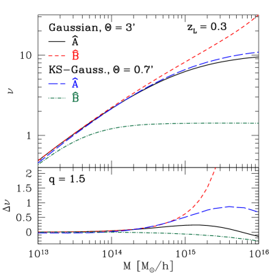
Figure 3.— Top panel: signal-to-noise of estimators $\hat{A}$ and $\hat{B}$ without lensing bias for a lens halo of mass $M$ at $z_{L}=0.3$, using a Gaussian shear filter and a KS-Gaussian filter (see Section 2.1). Bottom panel: Change in signal-to-noise of $\hat{A}$ and $\hat{B}$ induced by lensing bias, for the same filters and lensing halo.

When calculating the statistics of $\hat{B}$, we face the problem that $\langle\hat{A}/\hat{N}\rangle\neq\langle\hat{A}\rangle/\langle\hat{N}\rangle$ (see also paper I). However, we can employ this approximation if the effective number of galaxies used in the shear estimator, $\sim\bar{n}\Theta^{2}$ where $\Theta$ is the filter scale, is much larger than unity. In this case, we have for the expectation value

$$\langle\hat{B}\rangle=\frac{\langle\hat{A}\rangle}{\langle\hat{N}\rangle}=\frac{\int d^{2}\theta\>g(\vec{\theta})\mu^{q/2}(\vec{\theta})W(\vec{\theta})}{\int d^{2}\theta\>\mu^{q/2}(\vec{\theta})W(\vec{\theta})},$$ (28)

where we have again assumed that the shear is uncorrelated with source density. We see that the effect of lensing bias on $\hat{B}$ is partially canceled by the denominator, and therefore the expectation value for $\hat{B}$ is only weakly dependent on lensing bias corrections. In the absence of lensing bias and systematics, $\langle\hat{B}\rangle=\langle\hat{A}\rangle$.

When calculating the variance of $\hat{B}$ however, it is necessary to take into account the covariance between numerator and denominator. The full expression for ${\rm Var}(\hat{B})$ is derived in Appendix C, and is given in equation C4. The gist of it is that fluctuations in the number of source galaxies, due to both shot noise and source clustering, are partially canceled out (but see below). This becomes especially important for high masses, where the source clustering contribution to the variance begins to dominate. Finally, the large-scale structure variance is the same for both estimators, assuming that it is dominated by the weak lensing regime (lowest order in $\kappa$, $\gamma$).

The top panel of Fig. 3 shows the average expected signal-to-noise $\nu$, defined as $\nu=\langle\hat{A}\rangle/[{\rm Var}(\hat{A})]^{1/2}$ for both $\hat{A}$ and $\hat{B}$, as a function of halo mass. We have again assumed an NFW lensing halo, and we show results both for a Gaussian shear filter of width $\Theta=3^{\prime}$ and a KS-Gaussian filter with $\Theta=0.7^{\prime}$ (the choices of $\Theta$ will be justified in Section 2.5). Further, we have ignored lensing bias for the moment. For the Gaussian filter, we find that $\hat{B}$ is superior to $\hat{A}$ in terms of signal-to-noise for massive halos. For lower mass halos, where $g^{2}\ll\sigma_{e}^{2}$, both estimators are equivalent. Similar conclusions hold for the NFW-optimized filter.

The KS-Gaussian filter shows a very different behavior: here, $\hat{B}$ has significantly less signal-to-noise than $\hat{A}$ at all relevant masses (in fact, $\nu(\hat{B})$ never exceeds $\sim 1.4$), while $\hat{A}$ performs very similarly to the corresponding Gaussian estimator. The reason is that the covariance between the numerator and denominator of $\hat{B}$, which leads to the partial cancelation of fluctuations for the other shear filters, is strongly suppressed for a KS-Gaussian filter. This is a consequence of the inclusion of very large scales in the filter (see Appendix C). Without significant covariance between numerator and denominator, $\hat{B}$ is just the ratio of two noisy quantities, and not surprisingly has less signal-to-noise than $\hat{A}$. However, as mentioned in Section 2.1, this filter is commonly used on a pixelized shear map, rather than on the galaxies directly. Hence, Eq. (25) is actually not used with the KS-Gaussian filter in practice. Nevertheless, this result illustrates an important point: the choice of estimator (e.g., $\hat{A}$ vs $\hat{B}$) and filter function $W$ has to be done jointly, as the two are interrelated.

2.4. Impact of Lensing Bias

We now turn to the impact of lensing bias on $\hat{A}$ and $\hat{B}$. Lensing bias changes both the value (signal) of smoothed shear estimators, as well as the signal-to-noise. The latter effect is shown in the bottom panel of Fig. 3. Let us discuss the Gaussian filter first. We see that for $M\lesssim 3\times 10^{15}\,M_{\odot}/h$, lensing bias tends to increase the signal-to-noise in both estimators, an effect which increases with mass. The effect is in fact greater for $\hat{B}$ than for $\hat{A}$, even though the effect on the value of $\hat{B}$ is smaller. This is because lensing bias acts to decrease the variance of $\hat{B}$ in two ways: first, the increased source density reduces shot noise; second, lensing bias increases the covariance between numerator and denominator, improving the cancelation of fluctuations in the galaxy number above that without lensing bias. In case of $\hat{A}$, we see a reversal of the effect at very high masses: lensing bias in fact reduces the signal-to-noise of very high peaks for $\hat{A}$. This is because for very high halo masses (which are necessary to produce this high signal-to-noise), source clustering takes over as the dominant source at this filter scale. While the source clustering noise scales similarly with the lensing quantities as the signal itself ($\propto\mu^{q/2}g$), it is weighted by $W^{2}$ rather than $W$; this weighting favors smaller radii where the lensing magnification is stronger (see Fig. 8 in Appendix A), thus boosting the noise more than the signal. Note however that for such halos the optimal filter scale is significantly larger than the assumed 3 arcmin. On the other hand, fluctuations due to source clustering are largely canceled out in $\hat{B}$, and we do not see this reversal for this estimator. Instead, the boost in signal-to-noise grows strongly towards larger halo masses.

Again, the KS-Gaussian filter behaves differently: a significant increase in $\nu(\hat{A})$ is seen, while the effect on $\nu(\hat{B})$ is a small decrease. The causes for the differences are, for $\hat{A}$, that source clustering is somewhat smaller for the KS-Gaussian filter than for the Gaussian filter, and for $\hat{B}$, that lensing bias increases the variance of the estimator slightly faster than it increases the value of $\hat{B}$ itself.

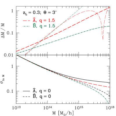
Figure 4.— Estimated mass bias when neglecting lensing bias (top) and relative error (bottom) on the mass measurement using filtered shear estimators $\hat{A}$ and $\hat{B}$. In the top panel, the thick lines show the mass bias expected if the signal itself is used to estimate the halo mass (thick lines), and if the signal-to-noise is used for the estimate (thin lines). In all cases, we have assumed a lens redshift of $z_{L}=0.3$, and a Gaussian shear filter with $\Theta=3^{\prime}$.

It is also interesting to consider what impact lensing bias has on the mass that one would assign to each shear peak. Assuming one can predict a relation $\hat{A}=\hat{A}(M)$, then from the amplitude of the shear peak one can estimate its mass. If, however, one fails to account for the boost in signal due to lensing bias, one will systematically overestimate the corresponding halo mass. The systematic mass offset is approximately given by

$$\frac{\Delta M_{\rm vir}}{M_{\rm vir}}=\frac{d\ln M}{d\ln\hat{A}}\frac{\Delta\hat{A}}{\hat{A}},$$ (29)

where the logarithmic slope $d\ln\hat{A}/d\ln M\approx 0.5-0.7$ depending on mass, and correspondingly for $\hat{B}$. The top panel of Fig. 4 (thick lines) shows the relative bias $\Delta M/M$ obtained with a Gaussian filter with $\Theta=3^{\prime}$. Clearly, for the most massive halos biases as large as tens of percent are possible. Note that the bias in $\hat{B}$ is smaller than that of $\hat{A}$. This is because we are only relying on the amplitude of $\hat{B}$ to estimate a cluster’s mass, and as we have seen, the amplitude of $\hat{B}$ is less affected than that of $\hat{A}$. The thin lines in the top panel of Fig. 4 show the expected bias if one would instead use the signal-to-noise of a lensing peak to estimate the halo mass, calculated using a similar relation to Eq. (29), but for $\nu(\hat{A}),\nu(\hat{B})$ instead $\hat{A},\hat{B}$. Here, the situation is reversed at high masses: the mass bias is larger for $\hat{B}$ than for $\hat{A}$, reaching order unity at $M\approx 10^{15}\,M_{\odot}/h$. Moreover, the bias in $\hat{A}$ changes sign at very high masses (for a fixed filter scale). This reflects the behavior of the lensing bias effect on $\nu$ seen in Fig. 3.

Turning now to the statistical uncertainty in the recovered mass, we have seen that lensing bias helps increase the signal-to-noise of a given halo. Thus, we expect properly accounting for lensing bias will reduce the statistical error in cluster mass estimates. The expected error in log-mass can be estimated as

$$\sigma_{\ln M}=\frac{d\ln M}{d\ln\hat{A}}\frac{1}{\nu_{A}}.$$ (30)

This is shown in the bottom panel of Fig. 4. Again, the improvement in mass resolution becomes relevant at the high-mass end. We also see how the better statistical performance of $\hat{B}$ over $\hat{A}$ for this filter reflects in the smaller mass uncertainty at the high-mass end. Note that this should only be seen as rough estimate; in practice, halo triaxiality and projection effects will increase the error in the recovered masses significantly.

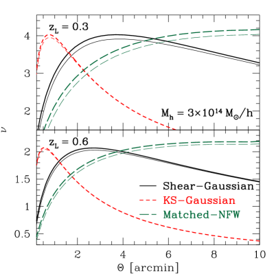
Figure 5.— Signal-to-noise of the estimator $\hat{A}$ as function of filter scale for different filter shapes (truncation scale in case of the matched NFW filter), for a $3\times 10^{14}\,M_{\odot}/h$ halo at two different redshifts: $z_{L}=0.3$ (top panel) and $z_{L}=0.6$ (bottom panel). The thin lines show results without lensing bias, while the thick lines include lensing bias ($q=1.5$).

2.5. Choice of Filter Scale

In order to optimize the filter shape, one has to adopt a metric with which different filtrs can be compared. In the following, we will focus on the goal of maximizing the signal-to-noise for a given lensing halo, which is most directly relevant to shear peak counts.

In order to test the relative performance of the different filters, we show the signal-to-noise $\nu$ for a $3\times 10^{14}\,M_{\odot}/h$ lensing halo at fixed lens redshifts of $z_{L}=0.3,\;0.6$ in Fig. 5, as a function of the filter scale $\Theta$. In case of the matched-NFW filter, $\Theta=\theta_{\rm max}$ is the truncation scale of the filter. We use $\hat{A}$ in all cases. The optimal signal-to-noise is determined by a balance between the signal $\hat{A}$, which decreases with increasing filter size, and the noise which also decreases. We see that all three filters peak at roughly the same signal-to-noise for $\hat{A}$, though the filter scale at which this peak is reached is very different. For the Gaussian filter, the optimal case is around $\Theta\approx 3^{\prime}$, which we have thus adopted as default value of the filter scale. For the KS-Gaussian, the optimal value is $\Theta\approx 0.7^{\prime}$. Note that these values depend on the mass and redshift of the lens.

The relative importance of the three noise contributions, shot noise, source clustering, and LSS noise, depends on the filter shape. In case of the KS-Gaussian filter, the LSS noise is much more significant, a factor of $\sim 10$ higher at the optimal filter scale than for the other two filters. Again, this is a consequence of the inclusion of very large scales in this filter. This will also be of relevance to the contribution of correlated large-scale structure to smoothed shear estimators.

Fig. 5 also shows the effect of lensing bias (thick lines vs thin lines): for this halo, lensing bias boosts the peak signal-to-noise by $\sim 5$% for the Gaussian and NFW-optimized filters. In case of the KS-Gaussian, the effect is slightly smaller, $\sim 3$%, due to the preference for large scales in that filter. Note that the optimal filter scale is moved to slightly smaller values by lensing bias. This is because the signal in $\hat{A}$ increases more steeply with decreasing filter size when including lensing bias.

Before deciding on an optimal filter, however, it is necessary to take into account the effect of associated and coincidental large-scale structure along the line of sight to the lens. Clearly, the likelihood of a chance superposition with unrelated matter concentrations with the filter scale (Hoekstra, 2003; Maturi et al., 2005). This might make a true optimal filter narrower than suggested by Fig. 5.

3. The Peak Function

We now turn to investigating the impact of lensing bias and filter choice on the abundance of detected shear peaks. To do so, we assume each shear peak corresponds to an NFW halo and that the peak position is the halo center. While in practice one expects some fraction of weak lensing peaks to arise due to chance superpositions of multiple halos, the results we obtain concerning how lensing bias impacts weak lensing peak finding should be indicative of the whole population.

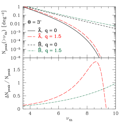
Figure 6.— Upper panel: Average number peak of peaks $N_{\rm peak}(>\nu_{\rm th})$ (per deg²) above the signal-to-noise threshold $\nu_{\rm th}$, with and without lensing bias for the two estimators $\hat{A}$, $\hat{B}$. We set $\Theta=3$ arcmin. Lower panel: Relative lensing bias effect on the peak counts, $\Delta N_{\rm peak}(>\nu_{\rm th})/N_{\rm peak}(\nu_{\rm th})$.

We estimate the average number of lensing peaks within a solid angle $\Omega_{s}$ above a given signal-to-noise threshold $\nu_{\rm th}$ as follows:

$$N_{\rm peak}(>\nu_{\rm th})=\> \Omega_{s}\int_{0}^{\infty}\frac{c\>dz_{L}}{H(z_{L})}\chi^{2}(z_{L})$$ (31)

$$\times\int_{\ln M_{\rm min}(z_{L},\nu_{\rm th})}^{\infty}d\ln M\>\frac{dn}{d\ln M}(z_{L},M),\quad$$

where $c$ is the speed of light, $H(z)$ is the Hubble expansion rate, $\chi(z)$ is the comoving distance to redshift $z$, $dn/d\ln M$ is the halo mass function, and $M_{\rm min}$ is defined via

$$\nu(M_{\rm min},z_{L})=\nu_{\rm th}.$$ (32)

Hence, lensing bias enters by lowering the effective $z$-dependent mass threshold of the survey, so that the number of peaks is increased. We use the fitting function of Tinker et al. (2008) to calculate $dn/d\ln M$ as function of mass and redshift from the linear matter power spectrum (recall that $M=M_{200m}$ throughout).

Fig. 6 shows the peak count statistics $N_{\rm peak}(>\nu_{\rm th})$ (peaks per deg²) with and without lensing bias using a Gaussian filter with fixed filter scale $\Theta=3$ arcmin. We also show the relative lensing bias effect $\Delta N_{\rm peak}/N_{\rm peak}$. Evidently, estimator $\hat{B}$ is more efficient at finding peaks for this filter, with or without lensing bias: the number of high signal-to-noise peaks ($\nu\gtrsim 6$) is higher than that found by $\hat{A}$ by orders of magnitude. Further, lensing bias can boost the weak lensing peak counts significantly for both $\hat{A}$ and $\hat{B}$, by more than a factor of 2 for high peaks. At high thresholds $\nu_{\rm th}\gtrsim 8.5$, we see a turnover, which reflects the trend seen in $\Delta\nu$ (Fig. 3).

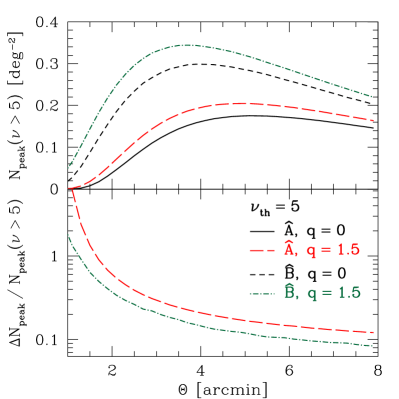
Figure 7.— Upper panel: Average number peak of peaks $N_{\rm peak}(\nu>5)$ (per deg²), with and without lensing bias for the two estimators $\hat{A}$, $\hat{B}$ as a function of the filter scale $\Theta$. Other survey specifications as in Fig. 2. Lower panel: Relative lensing bias effect on the peak counts, $\Delta N_{\rm peak}(\nu>5)/N_{\rm peak}(\nu>5)$.

Note that for very high peaks, i.e. massive halos, a filter scale of 3 arcmin is not optimal. Hence, it also interesting to consider the number of peaks above a fixed threshold as function of the filter width (Fig. 7). The different number of peaks here reflects the different mass thresholds for different filter scales at a fixed signal-to-noise threshold. Again, the location-normalized estimator $\hat{B}$ yields more peaks than $\hat{A}$, and lensing bias increases the number of $5\sigma$ shear peaks found with either estimator by $\sim$30%. Note that since lensing bias pushes the optimal filter scale to smaller values, the number of peaks increases faster with scale when incorporating the impact of lensing bias. Not surprisingly, we find that choosing smaller filters can increase the relative importance of lensing bias significantly (see the lower panel of Fig. 7).

Finally, we note that the result of the comparison $\hat{A}$ vs $\hat{B}$ reverses for the KS-Gaussian filter: $\hat{A}$ performs far better for this filter, as expected after Section 2.3.

4. Summary and Discussion

We have compared the expected signal-to-noise of the two most common types of filtered shear estimators for different filter functions, and studied how lensing bias impacts these estimators. In our signal-to-noise considerations, we also include the effects of the intrinsic clustering of source galaxies, and the variance of the estimators due to uncorrelated large-scale structure. The former noise contribution becomes important for massive lensing halos, while the latter’s importance only depends on the filter shape and scale considered.

We find that estimator and filter function need to be chosen jointly and cannot be regarded as independent. For example, for the Gaussian shear filter, the location-normalized estimator $(\hat{B})$ is statistically superior to the globally normalized estimator $(\hat{A})$ for high peaks. This is because fluctuations in the number of galaxies are canceled out to first order in $\hat{B}$. For the KS-Gaussian filter on the other hand, the situation is reversed: $\hat{A}$ performs far better than $\hat{B}$. According to our (certainly not exhaustive) results, a location-normalized estimator with a Gaussian-type shear filter appears to perform best statistically. The question of optimal filter+estimator combination certainly deserves more attention, as the abundance of high peaks can be suppressed by orders of magnitude for suboptimal choices (Fig. 6).

Another finding, of equal importance to their statistical properties, is that the two types of estimators respond very differently to uncertainties in the photometric redshifts (see the discussion in paper I). Specifically, the globally normalized estimator $\hat{A}$ does not suffer from the so-called dilution effect affecting $\hat{B}$, and should be much less sensitive to contamination of the source sample by galaxies associated with the lens.

Turning to lensing bias, we find that it affects both of the estimators we considered, and for all filter functions. While the signal-to-noise of either estimators can be boosted significantly (up to $\Delta\nu\sim 1-2$), the value of the estimator $\hat{A}$ is generally affected more strongly than that of $\hat{B}$. Indeed, if one were to estimate halo masses based solely on their smoothed shear signal, halo mass over-estimates as large as tens of percent are possible. Not surprisingly, the increase in signal-to-noise especially of high peaks also results in comparable boosts to the abundance of observed peaks. The magnitude of the effect depends strongly on the filter scale as well: smaller filter scales lead to a much larger boost in signal due to lensing bias, pushing the optimal filter scale towards smaller values.

While we have not considered the impact of halo triaxiality and correlated structures in our work, it is straightforward to understand how these can affect our conclusions. Specifically, both of these sources of noise tend to increase the weak lensing shear signal, and therefore will increase the relative importance of lensing bias. Moreover, if one wishes to minimize line-of-sight projections of multiple halos, we expect doing so will require smaller filters, resulting in a further increase of the importance of lensing bias.

In light of these results, it is clear that a proper modeling of lensing bias as well as source clustering will be a necessary component of cosmological interpretations of the shear peak function. Furthermore, these effects should also be taken into account when designing an optimal estimator+filter combination for shear peak finding. Fortunately, incorporating these two effects is fairly straightforward, both for analytic calculations and numerical studies with N-body simulations. Lensing bias, by increasing the signal-to-noise of the shear signal, has the potential to significantly boost the statistical power of shear selected samples of objects. Thus, properly accounting for lensing bias should allow us to maximize the cosmological potential of shear peak statistics.

Appendix A Lensing by an NFW halo

In this appendix we review our lens model used for the numerical results. The Navarro-Frenk-White density profile is given by (Navarro et al., 1997):

$$\rho(r)=\frac{\rho_{s}}{r/r_{s}(1+r/r_{s})^{2}},\quad\rho_{s}=\frac{M}{4\pi\>r_{s}^{3}[\ln(1+c)-c/(1+c)]},$$ (A1)

where $r_{s}$ is the scale radius, and $c=R_{200}/r_{s}$ is taken from the fit of Bullock et al. (2001). Note that this halo profile is not truncated at $R_{200}$. Actual halo profiles lie somewhere in between the extrapolated NFW profile adopted here and a truncated profile. The differences however appear mainly around $R_{200}$, which is typically larger than the filter size we will consider. Hence, the details of the outer halo profile do not change the results significantly.

Further, we make the small angle approximation. The lensing quantities $\kappa$ and $\gamma$ for an NFW halo have been derived in the literature (Oaxaca Wright and Brainerd (1999); Maturi et al. (2005)). For reference, the convergence at the scale radius is given by

$$\kappa_{s}=\frac{\rho_{s}r_{s}}{\Sigma_{\rm cr}}=\frac{3}{2}\frac{\rho_{s}r_{s}H_{0}^{2}}{\rho_{\rm cr,0}c^{2}}(1+z_{L})W_{L}(z_{L}).$$ (A2)

Here, $z_{L}$ is the halo redshift, $\rho_{\rm cr,0}$ is the critical density today, $c$ is the speed of light, and the lensing weight function is given by

$$W_{L}(z_{L})=\frac{c}{H(z_{s})}\int_{z_{L}}^{\infty}dz_{s}\frac{\chi_{L}}{\chi(z_{s})}[\chi(z_{s})-\chi_{L}]\frac{dN}{dz_{s}},$$ (A3)

where $\chi_{L}=\chi(z_{L})$, and $dN/dz$ is the normalized redshift distribution of the source galaxies, Eq. (1), determined from a fit to the expected redshift distribution of galaxies for DES (Annis, 2009).

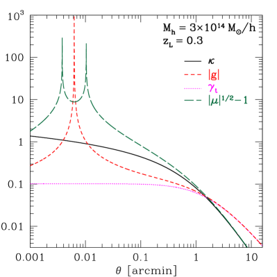
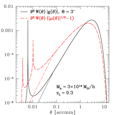
Figure 8.— Left panel: Profile of convergence $\kappa$, tangential shear $\gamma$, tangential reduced shear $g$ and scaled magnification $\sqrt{\mu}-1$ around a halo of mass $3\times 10^{14}\,M_{\odot}/h$ located at $z_{L}=0.3$. Right panel: Reduced shear and magnification weighted by area and the Gaussian filter $W$, for the same parameters as in the left panel. This shows which scales contribute to the signal in Eq. (2) and Eq. (25). The thin lines show the results capped at $\kappa=0.5$ (see text).

Fig. 8 (left panel) shows the profile of $\kappa$, $\gamma$, $g$ as well as $\mu$ for a typical detectable lensing halo at $z_{L}=0.3$. While $\kappa$, $\gamma$ are well-behaved, both $g$ and $\mu$ show the strong-lensing caustics, as expected. For this halo and source/lens redshifts, the strong-lensing regime defined by $g(\theta)\sim 1$ is relevant for $\theta\lesssim 0.05^{\prime}$. This regime cannot be treated by weak lensing analysis techniques, so it should be removed. Fortunately, the bulk of the signal-to-noise for weak lensing is at much larger radii. The right panel of Fig. 8 shows the relevant lensing quantities weighted by the Gaussian filter Eq. (12) for $\Theta=3$ arcmin. Clearly, the bulk of the signal comes from $\theta\sim 0.3-3$ arcmin, well outside the strong lensing regime for this halo. Although not of practical relevance, very massive halos do appear in the calculations where the strong lensing regime extends to beyond 0.2 arcmin. For those cases, we cap the convergence at $\kappa=0.5$. This is merely done to lead to convergence of the calculation, and only occurs for such high halo masses that it does not impact the results presented here.

Appendix B Large-scale structure variance

Here we re-derive the variance of $\hat{A}$ due to large scale structure in the survey (see Hoekstra, 2001). Since the bulk of the survey area will have small convergence, we can work in the weak-lensing limit, in which case $\hat{A}$ and $\hat{B}$ are equivalent. Furthermore, we only calculate the leading contribution from the power spectrum of the lensing field, neglecting higher order moments which in principle can become relevant on very small scales. The computation is most conveniently done in Fourier space. For this, we first rewrite Eq. (6) in the weak lensing limit ($g=\gamma$) as as an expression for the filtered convergence $\kappa$ (e.g., Bartelmann and Schneider, 2001):

$$\hat{A}(\vec{\theta}) = \int d^{2}\theta^{\prime}\kappa(\vec{\theta}^{\prime})W^{\kappa}(|\vec{\theta}-\vec{\theta}^{\prime}|)$$ (B1)

$$W^{\kappa}(\theta) = 2\int_{\theta}^{\infty}\frac{d\theta^{\prime}}{\theta^{\prime}}W(\theta^{\prime})-W(\theta).$$ (B2)

Note the non-local relationship between the shear filter and the corresponding convergence filter. Since $\kappa$ is a scalar quantity, Eq. (B1) can be straightforwardly written in Fourier space:

$$\tilde{A}(\vec{\ell})=\tilde{\kappa}(\vec{\ell})\tilde{W}^{\kappa}(\ell),$$ (B3)

where tilded quantities stand for Fourier transforms:

$$\tilde{X}(\vec{\ell})=\int d^{2}\theta\>e^{i\vec{\ell}\cdot\vec{\theta}}X(\vec{\theta}).$$ (B4)

Then, using the definition of the angular power spectrum of the convergence:

$$\langle\kappa(\vec{\ell})\kappa(-\vec{\ell}^{\prime})\rangle=(2\pi)^{2}\delta_{D}(\vec{\ell}-\vec{\ell}^{\prime})C^{\kappa}(\ell),$$ (B5)

we can write the first-order variance of $\hat{A}$ as:

$$\sigma^{2}_{\rm LSS}=\langle\hat{A}^{2}\rangle=\int\frac{d^{2}\ell}{(2\pi)^{2}}|\tilde{W}^{\kappa}(\ell)|^{2}\>C^{\kappa}(\ell).$$ (B6)

This quantity is shown as dotted line in Fig. 2, for a Gaussian shear filter Eq. (12) (note that $W^{\kappa}$ for this filter is not a Gaussian). It is also straightforward to calculate the leading lensing bias correction to $\sigma_{\rm LSS}$, following the second order correction to $C^{\kappa}(\vec{\ell})$ presented in Schmidt et al. (2009b). While we include this correction, the relative change of $\sigma_{\rm LSS}$ only amounts to a few percent for filter scales $\Theta\gtrsim 1^{\prime}$ (see also White (2005)).

Appendix C Variance of the location-normalized estimator

In this section, we derive the variance of $\hat{B}$ due to shot noise and source clustering, taking into account the covariance between numerator and denominator. We expand $\hat{B}=\hat{A}/\hat{N}$ around its expectation value, $\langle\hat{B}\rangle=\langle\hat{A}\rangle/\langle\hat{N}\rangle$, assuming that fluctuations are much smaller than unity (justified if $\bar{n}\,\Theta^{2}\gg 1$). In close analogy to the derivation in the appendix of paper I, this yields

$$\frac{{\rm Var}(\hat{B})}{\langle\hat{B}\rangle^{2}}=\frac{{\rm Var}(\hat{A})}{\langle\hat{A}\rangle^{2}}+3\frac{{\rm Var}(\hat{N})}{\langle\hat{N}\rangle^{2}}-4\frac{{\rm Cov}(\hat{A},\hat{N})}{\langle\hat{A}\rangle\langle\hat{N}\rangle},$$ (C1)

where

$${\rm Cov}(\hat{A},\hat{N})\equiv\langle\hat{A}\hat{N}\rangle-\langle\hat{A}\rangle\langle\hat{N}\rangle = \frac{1}{\bar{n}}\int d^{2}\theta\>W^{2}(\theta)\mu^{q/2}(\theta)g(\theta)+\int d^{2}\theta\int d^{2}\theta^{\prime}\>W\mu^{q/2}W^{\prime}\mu^{\prime q/2}g^{\prime}\xi(|\vec{\theta}^{\prime}-\vec{\theta}|)$$ (C2)

$${\rm Var}(\hat{N}) = \frac{1}{\bar{n}}\int d^{2}\theta\>W^{2}(\theta)\mu^{q/2}(\theta)+\int d^{2}\theta\int d^{2}\theta^{\prime}\>W\mu^{q/2}W^{\prime}\mu^{\prime q/2}\xi(|\vec{\theta}-\vec{\theta}^{\prime}|).\quad$$ (C3)

Here, we have used the shorthand notation introduced after Eq. (24). In each of these equations, the first term denotes the shot noise contribution, while the second is the contribution from source clustering. We see from Eq. (C1) that there is a cancelation of noise terms (both shot noise and source clustering) due to the positive covariance between $\hat{A}$ and $\hat{N}$. The cancelation is not perfect, since the various terms involve different integrals over shear and magnification. However, for relatively low-mass halos for which $g^{2}\ll\sigma_{e}^{2}$, the shot noise term of ${\rm Var}(\hat{A})$ [Eq. (22)] dominates in Eq. (C1). In this limit, we recover ${\rm Var}(\hat{B})={\rm Var}(\hat{A})$ (see Fig. 3).

If we neglect lensing bias and source clustering in both $\hat{B}$ and $\hat{A}$, so that $\langle\hat{A}\rangle=\langle\hat{B}\rangle$, Eq. (C1) simplifies to

$${\rm Var}(\hat{B})={\rm Var}(\hat{A})+\frac{\langle\hat{A}\rangle^{2}}{\bar{n}\>\mathcal{A}}\left(3-4\frac{\mathcal{A}\int d^{2}\theta\>W^{2}g}{\int d^{2}\theta\>W\>g}\right),$$ (C4)

where we have defined $\mathcal{A}=1/\int d^{2}\theta\>W^{2}$ as the effective filter area. If the shear $g$ was constant, then the last term in Eq. (C4) would evaluate to 4, canceling the $g^{2}$ term in ${\rm Var}(\hat{A})$ [Eq. (22)] and leading to ${\rm Var}(\hat{B})=\sigma_{e}^{2}/(2\bar{n}\,\mathcal{A})$. Eq. (C4) makes it clear that the last term determines whether $\hat{B}$ performs better or worse than $\hat{A}$: if $\mathcal{A}\int W^{2}g/\int W\,g$ is order unity, ${\rm Var}(\hat{B})<{\rm Var}(\hat{A})$. If it is much less than 1, ${\rm Var}(\hat{B})$ can be significantly larger than ${\rm Var}(\hat{A})$. The latter is the case for the KS-Gaussian filter, where $\mathcal{A}\int W^{2}g/\int W\,g\approx 0.2-0.3$, due to the preferential weighting of very large scales. Similar reasoning applies to the source clustering contribution. This explains why $\hat{B}$ performs worse than $\hat{A}$ for the KS-Gaussian filter. Note that this effect will be mitigated when employing this filter on a pixelized shear map: since the sum in Eq. (25) now only runs over galaxies within a small pixel (with $W=1$) instead of running over all galaxies, there will be significant covariance between numerator and denominator, reducing the noise in the pixelized shear.

References

- Rozo et al. (2010a) E. Rozo, H. Wu, and F. Schmidt, ApJ submitted (2010a).
- Vikhlinin et al. (2009) A. Vikhlinin, A. V. Kravtsov, R. A. Burenin, H. Ebeling, W. R. Forman, A. Hornstrup, C. Jones, S. S. Murray, D. Nagai, H. Quintana, et al., ApJ 692, 1060 (2009), 0812.2720.
- Rozo et al. (2010b) E. Rozo, R. H. Wechsler, E. S. Rykoff, J. T. Annis, M. R. Becker, A. E. Evrard, J. A. Frieman, S. M. Hansen, J. Hao, D. E. Johnston, et al., ApJ 708, 645 (2010b), 0902.3702.
- Mantz et al. (2009) A. Mantz, S. W. Allen, D. Rapetti, and H. Ebeling, ArXiv e-prints (2009), 0909.3098.
- Henry et al. (2009) J. P. Henry, A. E. Evrard, H. Hoekstra, A. Babul, and A. Mahdavi, ApJ 691, 1307 (2009), 0809.3832.
- Vanderlinde et al. (2010) K. Vanderlinde, T. M. Crawford, T. de Haan, J. P. Dudley, L. Shaw, P. A. R. Ade, K. A. Aird, B. A. Benson, L. E. Bleem, M. Brodwin, et al., ArXiv e-prints (2010), 1003.0003.
- Schneider (1996) P. Schneider, MNRAS 283, 837 (1996), arXiv:astro-ph/9601039.
- Hennawi and Spergel (2005) J. F. Hennawi and D. N. Spergel, ApJ 624, 59 (2005), arXiv:astro-ph/0404349.
- Hamana et al. (2004) T. Hamana, M. Takada, and N. Yoshida, MNRAS 350, 893 (2004), arXiv:astro-ph/0310607.
- Miyazaki et al. (2007) S. Miyazaki, T. Hamana, R. S. Ellis, N. Kashikawa, R. J. Massey, J. Taylor, and A. Refregier, ApJ 669, 714 (2007), 0707.2249.
- Wittman et al. (2006) D. Wittman, I. P. Dell’Antonio, J. P. Hughes, V. E. Margoniner, J. A. Tyson, J. G. Cohen, and D. Norman, ApJ 643, 128 (2006), arXiv:astro-ph/0507606.
- Gavazzi and Soucail (2007) R. Gavazzi and G. Soucail, A&A 462, 459 (2007), arXiv:astro-ph/0605591.
- Wang et al. (2009) S. Wang, Z. Haiman, and M. May, ApJ 691, 547 (2009), 0809.4052.
- Dietrich and Hartlap (2009) J. P. Dietrich and J. Hartlap, ArXiv e-prints (2009), 0906.3512.
- Kratochvil et al. (2009) J. M. Kratochvil, Z. Haiman, and M. May, ArXiv e-prints (2009), 0907.0486.
- Marian et al. (2010) L. Marian, R. E. Smith, and G. M. Bernstein, ApJ 709, 286 (2010), 0912.0261.
- Broadhurst et al. (1995) T. J. Broadhurst, A. N. Taylor, and J. A. Peacock, Astrophys. J. 438, 49 (1995), astro-ph/9406052.
- Schmidt et al. (2009a) F. Schmidt, E. Rozo, S. Dodelson, L. Hui, and E. Sheldon, Physical Review Letters 103, 051301 (2009a), 0904.4702.
- Schneider et al. (2000) P. Schneider, L. King, and T. Erben, A&A 353, 41 (2000), arXiv:astro-ph/9907143.
- Van Waerbeke et al. (2010) L. Van Waerbeke, H. Hildebrandt, J. Ford, and M. Milkeraitis, ArXiv e-prints (2010), 1004.3793.
- Maturi et al. (2005) M. Maturi, M. Meneghetti, M. Bartelmann, K. Dolag, and L. Moscardini, A&A 442, 851 (2005), arXiv:astro-ph/0412604.
- van Waerbeke (2000) L. van Waerbeke, MNRAS 313, 524 (2000), arXiv:astro-ph/9909160.
- Schneider et al. (1997) P. Schneider, L. van Waerbeke, B. Jain, and G. Kruse (1997), astro-ph/9708143.
- Marian and Bernstein (2006) L. Marian and G. M. Bernstein, Phys. Rev. D 73, 123525 (2006), arXiv:astro-ph/0605746.
- Kaiser and Squires (1993) N. Kaiser and G. Squires, ApJ 404, 441 (1993).
- Navarro et al. (1996) J. F. Navarro, C. S. Frenk, and S. D. M. White, ApJ 462, 563 (1996), arXiv:astro-ph/9508025.
- Schmidt et al. (2009b) F. Schmidt, E. Rozo, S. Dodelson, L. Hui, and E. Sheldon, ApJ 702, 593 (2009b), 0904.4703.
- Smith et al. (2003) R. E. Smith, J. A. Peacock, A. Jenkins, S. D. M. White, C. S. Frenk, F. R. Pearce, P. A. Thomas, G. Efstathiou, and H. M. P. Couchman, MNRAS 341, 1311 (2003), arXiv:astro-ph/0207664.
- Matsubara (2000) T. Matsubara, ApJ 537, L77 (2000), arXiv:astro-ph/0004392.
- Hui et al. (2007) L. Hui, E. Gaztañaga, and M. LoVerde, Phys. Rev. D 76, 103502 (2007), arXiv:0706.1071.
- Hoekstra (2001) H. Hoekstra, A&A 370, 743 (2001), arXiv:astro-ph/0102368.
- Bernardeau (1998) F. Bernardeau, A&A 338, 375 (1998), arXiv:astro-ph/9712115.
- Medezinski et al. (2007) E. Medezinski, T. Broadhurst, K. Umetsu, D. Coe, N. Benítez, H. Ford, Y. Rephaeli, N. Arimoto, and X. Kong, ApJ 663, 717 (2007), arXiv:astro-ph/0608499.
- Hoekstra (2003) H. Hoekstra, MNRAS 339, 1155 (2003), arXiv:astro-ph/0208351.
- Tinker et al. (2008) J. Tinker, A. V. Kravtsov, A. Klypin, K. Abazajian, M. Warren, G. Yepes, S. Gottlöber, and D. E. Holz, ApJ 688, 709 (2008), 0803.2706.
- Navarro et al. (1997) J. F. Navarro, C. S. Frenk, and S. D. M. White, Astrophys. J. 490, 493 (1997), astro-ph/9611107.
- Bullock et al. (2001) J. S. Bullock, T. S. Kolatt, Y. Sigad, R. S. Somerville, A. V. Kravtsov, A. A. Klypin, J. R. Primack, and A. Dekel, MNRAS 321, 559 (2001), arXiv:astro-ph/9908159.
- Oaxaca Wright and Brainerd (1999) C. Oaxaca Wright and T. G. Brainerd, ArXiv Astrophysics e-prints (1999), arXiv:astro-ph/9908213.
- Annis (2009) J. Annis (2009), private communication.
- Bartelmann and Schneider (2001) M. Bartelmann and P. Schneider, Phys. Rep. 340, 291 (2001), arXiv:astro-ph/9912508.
- White (2005) M. White, Astroparticle Physics 23, 349 (2005).