The UV galaxy Luminosity Function at $z$=3-5 from the CFHT Legacy Survey Deep fields

Abstract

Aims. We measure and study the evolution of the UV galaxy Luminosity Function (LF) at $z$=3-5 from the largest high-redshift survey to date, the Deep part of the CFHT Legacy Survey. We also give accurate estimates of the SFR density at these redshifts.

Methods. We consider $\sim$ 100 000 Lyman-break galaxies at $z\approx$ 3.1, 3.8 & 4.8 selected from very deep $ugriz$ images of this data set and estimate their rest-frame 1600$\rm{\AA}$ luminosity function. Due to the large survey volume, cosmic variance plays a negligible role. Furthermore, we measure the bright end of the LF with unprecedented statistical accuracy. Contamination fractions from stars and low-$z$ galaxy interlopers are estimated from simulations. From these simulations the redshift distributions of the Lyman-break galaxies in the different samples are estimated, and those redshifts are used to choose bands and calculate k-corrections so that the LFs are compared at the same rest-frame wavelength. To correct for incompleteness, we study the detection rate of simulated galaxies injected to the images as a function of magnitude and redshift. We estimate the contribution of several systematic effects in the analysis to test the robustness of our results.

Results. We find the bright end of the LF of our $u$-dropout sample to deviate significantly from a Schechter function. If we modify the function by a recently proposed magnification model, the fit improves. For the first time in an LBG sample, we can measure down to the density regime where magnification affects the shape of the observed LF because of the very bright and rare galaxies we are able to probe with this data set. We find an increase in the normalisation, $\phi^{*}$, of the LF by a factor of 2.5 between $z\approx 5$ and $z\approx 3$. The faint-end slope of the LF does not evolve significantly between $z\approx 5$ and $z\approx 3$. We do not find a significant evolution of the characteristic magnitude in the studied redshift interval, possibly because of insufficient knowledge of the source redshift distribution. The SFR density is found to increase by a factor of $\sim$2 from $z\approx 5$ to $z\approx 4$. The evolution from $z\approx 4$ to $z\approx 3$ is less eminent.

1 Introduction

The formation and evolution of galaxies rank among the big questions in astronomy and still await a complete explanation. According to current theory, the formation of dark matter haloes by gravitational instabilities is an essential first step in the formation of galaxies (Eggen et al. 1962). Stars are believed to form when gas cools at the centres of these haloes (White & Rees 1978), and make up the part of the galaxy that we can observe. A number of physical processes strongly affect this baryonic mass assembly, like the hydrodynamics of the gas, feedback processes by supernovae and stellar winds, possibly magnetic fields, the role of AGN, or the effects of galaxy-galaxy interactions and mergers. For these reasons the modelling of galaxy formation depends on many free parameters and is not very well constrained.

Over the past decade the high redshift universe has become accessible observationally through the use of photometric techniques. By detection of the spectral discontinuity due to the redshifted Lyman-break in a multi-wavelength filter set, large and clean samples of high redshift star-forming galaxies can be selected (Steidel et al. 1996, 1999; Giavalisco 2002), with low amounts of contamination. These samples can be used to study several properties of the early universe. For example, by measuring the correlation function of these Lyman-break Galaxies (LBGs) and comparing it with the correlation of dark matter, the characteristic mass of their haloes can be determined (e.g. Giavalisco & Dickinson 2001; Ouchi et al. 2004b; Hildebrandt et al. 2005, 2007, 2009). Hubble Space Telescope observations of LBGs are used to study how certain morphological types evolve with time (Pirzkal et al. 2005). A study of the evolution of the UV Luminosity Function (LF) (Steidel et al. 1996, 1999; Sawicki & Thompson 2006; Bouwens et al. 2007), which is the measure of the number of galaxies per unit volume as a function of luminosity, is another fundamental probe in galaxy formation and evolution, because of its close relation to star formation processes.

Several techniques can be used to estimate the star formation rate (SFR) in galaxies, mostly based on the existence of massive, young stars, indicative of recent star formation. A commonly used way to probe the existence of massive stars is the H$\alpha$ luminosity (Kennicutt 1983), because H$\alpha$ photons originate from the gas ionized by the radiation of massive stars. A second star formation indicator is the infrared (IR) luminosity originating from dust continuum emission (Kennicutt 1998; Hirashita et al. 2003). The absorption cross section of dust is strongly peaked in the UV, and therefore the existence of UV emitting, i.e. massive, stars is probed indirectly. Thirdly, the UV continuum is used as a star formation probe, with the main advantages being that the UV-emission of the young stellar population is $directly$ observed, unlike in H-$\alpha$ and IR studies. Furthermore, this technique can be applied from the ground to star-forming galaxies over a wide range of redshifts. Hence, it is still the most powerful probe of cosmological evolution of the SFR (Madau et al. 1996). However, information about the initial mass function (IMF), and particularly the extinction by dust are required to estimate the total star formation rate.

In this paper we estimate the UV LF at redshifts $z$=3-5 from the Canada-France-Hawaii-Telescope Legacy Survey (CFHTLS) Deep, a survey covering 4 square degrees in four independent fields spread across the sky. Since our samples, at different redshifts, are all extracted from the same dataset, this gives an excellent opportunity to study a possible evolution of the LF in this redshift interval. Several systematic effects that need to be considered when comparing results at different redshifts from different surveys (e.g. source extraction, masking, PSF-modelling, etc.) can be avoided when the different redshift samples are extracted from the same survey. Due to the large volumes we probe with our 4 square degree survey, the influence of cosmic variance on the shape of the estimated LF is negligible (Trenti & Stiavelli 2008), as we expect cosmic variance to affect our number counts only at the 1-5% level (Somerville et al. 2004). We can study the bright end of the LF with unprecedented accuracy, as these objects are rare and we are able to measure down to very low densities. This allows us to study the effect that magnification has on the observed distribution (see recent results by Jain & Lima 2010), and study a possible deviation from the commonly used Schechter function. Furthermore, given the depth of the stacked images, we can probe the faint end of the luminosity function with comparable precision as the deepest ground based surveys have done before (Sawicki & Thompson 2006).

The structure of this paper is as follows: In Sect. 2 we describe the data set we use, the LBG selection criteria as well as the simulations that lead to the redshift distributions and contamination fractions. In Sect. 3 the survey’s completeness and the effective survey volumes are estimated. In Sect. 4 we proceed with the resulting estimated LFs, present the best-fitting Schechter parameters, and show how a simple magnification model can significantly improve the quality of the fit. The UV luminosity densities (UVLD) and SFR densities (SFRD) are estimated based on the measured LFs. We also elaborate on the robustness of our results. In Sect. 5 we compare these to previous determinations of the UV LF and SFRD from the literature. In Sect. 6 we finish with a summary and present our conclusions.

We use the AB magnitudes system (Oke & Gunn 1983) throughout and adopt $\Lambda$CDM cosmology with $\rm{\Omega_{m}=0.3}$, $\rm{\Omega_{\Lambda}=0.7}$ and $\rm{H_{0}=70\,km\,s^{-1}\,Mpc^{-1}}$.

2 Data & Samples

2.1 The CFHT Legacy Survey Deep

For this work we make use of publicly available data from the CFHTLS Deep, a survey using MegaCam mounted at the prime focus of the CFHT which covers four independent fields of 1 square degree each. Images are taken in the filters $ugriz$ and are pre-processed using the Elixir system (Magnier & Cuillandre 2004). Image reduction is done using the THELI pipeline (Erben et al. 2005; Hildebrandt et al. 2006), leading to approximate $5\sigma$ point source limits of 27.5, 27.9, 27.9, 27.7 and 26.5 for the $ugriz$ bands, respectively. The limits for each of the fields lie within 0.2 mag from these average values.

Source Extractor (Bertin & Arnouts 1996) is used to create a multi-colour catalogue. Total $i$-band magnitudes are measured in Kron-like apertures (Kron 1980) using SExtractor’s AUTO magnitudes. Every image is smoothed by convolution with a Gaussian filter to match the seeing of the image with the worst seeing value (typically the $u$-band). These corrections are typically small - all bands have a seeing below 1 arcsec. The dual-image mode of SExtractor is then used with the unconvolved $i$-band for source detection and isophotal magnitudes from the convolved bands to estimate colours. An extensive description of the data reduction and catalogue creation is given in Erben et al. (2009) and Hildebrandt et al. (2009).

2.2 $u$-, $g$-, and $r$-dropout samples

Clean samples of $u$-, $g$-, and $r$-dropouts are selected based on the following selection criteria (Hildebrandt et al. 2009):

$$u\rm{-dropouts} : 1.0<(u-g)\land-1.0<(g-r)<1.2\land$$ (1)

$$1.5\cdot(g-r)<(u-g)-0.75,$$

$$g\rm{-dropouts} : 1.0<(g-r)\land-1.0<(r-i)<1.0\land$$ (2)

$$1.5\cdot(r-i)<(g-r)-0.80,$$

$$r\rm{-dropouts} : 1.2<(r-i)\land-1.0<(i-z)<0.7\land$$ (3)

$$1.5\cdot(i-z)<(r-i)-1.00.$$

Furthermore, it is required that all LBGs have a $SExtractor$ CLASS_STAR parameter of CLASS_STAR $<$ 0.9, that $g$-dropouts are not detected in $u$, and that $r$-dropouts are neither detected in $u$ nor in $g$. Note that the colour selection criteria of the $u$-dropout sample in Hildebrandt et al. (2009) are pretty conservative. We relaxed the $u-g$ cut slightly to make the selection more comparable to e.g. Steidel et al. (2003), Steidel et al. (2004) and Sawicki & Thompson (2006).

This results in the selection of 50880 $u$-, 36226 $g$-, and 11411 $r$-dropouts in total over the four fields. Their magnitude distributions are shown in Fig. 1. Note the differences in depth of the individual fields.

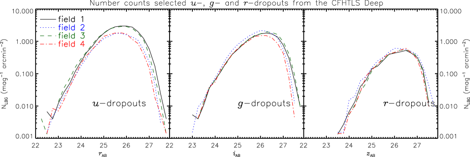
Figure 1: From left to right the number counts of the u-, g-, and r-dropouts in the CFHTLS Deep, as selected by the colour criteria of Eqs. 1-3.

2.3 Redshift distributions & Contamination fractions

The majority of the selected sources is too faint to make a spectroscopic redshift determination possible, and the brighter candidates have not spectroscopically been observed yet. For this reason Hildebrandt et al. (2009) estimated the redshift distributions by means of photometric redshifts and simulations.

Throughout this paper we will use the mean redshift values from simulations based on synthetic templates by Bruzual A. & Charlot (1993), being $<z>\cong$ 3.1, 3.8 and 4.7 for the $u$-, $g$-, and $r$-dropouts respectively. We estimate the uncertainty in the mean redshifts to 0.1 for the three dropout samples.

In order to address the amount of contamination in our LBG samples, Hildebrandt et al. (2009) consider the possibilities of stars and low-$z$ galaxies scattering in the selection boxes. Galaxies are simulated based on templates from the library of Bruzual A. & Charlot (1993), while the colours of stars in the fields are estimated based on the TRILEGAL galactic model (Girardi et al. 2005). Contamination fractions are shown graphically in Fig. 2.

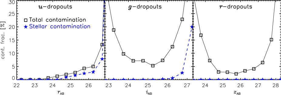
Figure 2: Contamination fractions of stars and low-$z$ galaxies in the dropout samples. Blue $\star$-symbols connected by a dashed line show the stellar contamination fraction based on a galactic model. Black squares connected by the solid line show the total contamination fraction from Hildebrandt et al. (2009).

Stellar contamination is negligible for the brighter objects, as the selection boxes steer away from the stellar locus. For faint objects in the $u$-, and $g$-dropout samples, the stellar contamination increases as a result of photometric scatter.

The contamination by low-$z$ galaxies is negligible in the $u$-dropout sample, as the Lyman break for a $z\sim 3$ galaxy is still blue-ward of the $z\sim 0$ Balmer/4000$\rm{\AA}$ break. For higher redshifts this ceases to be the case, so that the $g$-, and $r$-dropout samples suffer from a significant contamination fraction at the bright end, where the LBG population is sparse. Faint low-$z$ objects are likely to scatter into the selection box in each of the samples, so that the contamination fractions are increased here.

Since the contamination fractions are low at the bright end of the $u$-dropouts, we have the potential to probe the LF to very low LBG galaxy densities. We inspect the 80 brightest objects ($r_{\rm{AB}}<23.2$) in the $u$-dropout sample by eye and remove obvious spurious sources, 30 in total. A strong, but certainly slightly subjective, rejection criterion is the size of the region in which the flux is measured, i.e. the half-light radius (13 objects rejected). Sources that are clearly blended by a bright neighbour (2 objects), as well as sources that have a too large apparent size (3 objects). Also an asteroid track has been removed.

In the $g$-, and $r$-dropout sample we do not probe these low ($\lesssim 0.01\,\rm{mag^{-1}\,arcmin^{-2}}$) LBG galaxy densities, since these points are unreliable due to the high contamination fractions from low-$z$ objects (see Fig. 2). This prohibits a study of the bright end of the LF for the $g$-, and $r$-dropouts until the nature of the individual sources has been verified.

3 Analysis - Survey completeness

We use a detailed modelling approach to estimate the completeness of the survey as a function of magnitude and redshift, for each of the dropout samples. We add artificial objects to our images, with colours representative of star-forming galaxies, and try to recover them following the same source extraction and colour selection criteria as for the real data. We investigate how the increasing scatter in the colours for fainter objects influences the completeness as a function of magnitude. Furthermore, one expects that, for fainter dropout objects, the redshift distribution of these objects broadens due to the same effect. Hence we will also model this as a function of redshift.

We describe our fiducial model SEDs, sizes and shapes of the simulated objects below. The assumptions we make, are tested in Sect. 4.3 to estimate the robustness of the results.

3.1 Model galaxies

The Bruzual A. & Charlot (1993) stellar population synthesis library is used to set up our fiducial galaxy SED model; a 100 Myr old galaxy template with constant star formation. A Miller & Scalo (1979) IMF is assumed. The optical depth of neutral hydrogen, as a function of redshift, is modelled according to Madau (1995).

This template is reddened by the starburst extinction law from Calzetti et al. (2000), with a distribution in $E(B-V)$. This distribution we choose such that the UV-continuum slopes that we measure from the data are matched when we use our fiducial template as a base. To measure the UV-continuum slopes, we use a colour redward of 1600$\AA$ rest-frame, i.e. the $r-i$ colour for the $u$-dropouts and the $i-z$ colour for the $g$-dropouts. For the $r$-dropouts we can not perform a similar measurement because we do not have observations in a band redward of the $z$-band. Therefore we will use the same distribution of dust as we find for the $g$-dropouts.

For the $u$-dropouts we find that a uniform dust distribution with reddening between with 0.1$<E(B-V)<$0.4 gives a good fit to the data, see Fig. 3. For the $g$-dropouts we measure a larger spread in UV-continuum slopes, and find a reasonable fit when using a uniform dust distribution with reddening between 0.0$<E(B-V)<$0.5. It should be noted that the age and amount of dust attenuation of the template are highly degenerate, so that different combinations of these parameters fit the UV-continuum slopes in the data. It is especially important to correctly match the distribution of the UV-continuum slopes from the data with the model galaxies, since an increase (decrease) in the age of the galaxy model template has a similar effect on the LF as an increase (decrease) of the amount of dust. We will elaborate on this in Sect. 4.3. If we measure the UV-continuum slopes in our data for different magnitude bins, we do not find a significant evolution. Therefore we will use a distribution of dust attenuation in our simulations that is independent of magnitude.

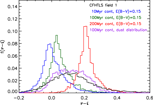
Figure 3: The distribution of UV-continuum slopes for the $u$-dropouts as measured by the $r-i$ colour from the CFHT data (black) compared with the outcomes from simulations. The colour is measured in a part of the spectrum without strong features, redward of 1600$\AA$. Both an older template and a higher amount of dust result in a redder UV colour. The amount of dust we need to add therefore depends on the age of the base template. For the $u$-dropouts we find that a uniform distribution of dust with 0.1$<E(B-V)<$0.4 gives a good fit to the data, when the template is 100 Myr old with a constant amount of star formation (purple).

LBGs have typical half-light radii of $r_{1/2}\sim$ 0.1”-0.3” (Giavalisco et al. 1996) and thus are unresolved by the CFHT and can be treated as point sources. As the size of the PSF in the CFHT images is strongly position dependent, we have to adapt the injected sources accordingly. We parametrize the PSF by a Moffat profile,

$$I=I_{0}\left[1+(2^{1/\beta}-1)\cdot\left(\frac{R}{R_{0}}\right)^{2}\right]^{-\beta},$$ (4)

in which $\beta$ and $R_{0}$ are the parameters that we adapt to adjust the shape and size of the profile respectively. $I_{0}$ represents the flux normalisation.

In order to measure the PSF as a function of position for the different filters and fields, we first select several hundred stars based on their magnitudes and half-light radii, in each field and each filter. We measure the 50% and 90% flux radii of these stars, $\rm{r_{50}}$ and $\rm{r_{90}}$, using SExtractor. The ratio of these flux radii uniquely determines the Moffat-$\beta$ parameter, which, in combination with either one of the flux radii, gives the Moffat profile radius $R_{0}$ for each star. We find that the Moffat-$\beta$ parameter is fairly constant over the fields and filters $(\beta\approx 4.0)$ and only $R_{0}$ changes significantly. To model $R_{0}$ as a function of position, we fit a 2-dimensional polynomial function to the SExtracted values for $r_{50}$. This constrains the PSF size on every position, for every field and filter.

We find that there is a $\sim$30% difference in $R_{0}$ between the image center and boundaries. As this, in our ground-based wide-field survey, is by far the dominating effect in the apparent surface brightnesses of our sources, we do not assume an intrinsic size distribution for the sources in the main simulations of this paper.

3.2 Eddington bias

If we consider a certain intrinsic magnitude distribution of galaxies, the recovered distribution after source extraction and colour selection will look different due to statistical fluctuations in the measurement. In our analysis we attempt to correct for this effect called Eddington bias (Eddington 1913; Teerikorpi 2004). It is hard to estimate this bias analytically because the size of the magnitude scatter is an increasing function of magnitude. Also, when approaching the completeness limit of the survey, only the brighter objects will be detected. What generally happens is that intrinsically faint objects will on average look brighter than they are.

The Eddington bias can be estimated by comparing the intrinsic magnitudes of the injected sources to the recovered magnitudes. Such a comparison is shown in Fig. 4, stressing the importance of that effect for faint magnitudes.

We want to inject sources with the same magnitude distribution as the intrinsic distribution, to get an unbiased result. As the bias is expected to be largest for fainter sources, it is especially important to correctly model the faint-end of the intrinsic distribution. Here we adopt a LF that is consistent with the deepest LBG survey, conducted by Bouwens et al. (2007).

Figure 4: The difference between recovered and injected source magnitudes as a function of recovered magnitude for the $r$-dropouts. Similar trends appear in the other dropout samples. The error bars reflect the scatter from the four fields. A similar effect as shown around $\rm{m_{rec}}=25.3$, namely an increase of $\rm{m_{rec}-m_{inj}}$, is found by Bouwens et al. (2006, Fig.19), where observations were used rather than simulations.

3.3 Source injection and recovery

Following this adopted intrinsic distribution we inject $20\,000$ sources in each of the images, for 60 equal redshift steps between $z=0.0$ and $z=6.0$. To verify that the injected sources do not significantly influence each other by blending, nor that the background is influenced significantly, we perform the following tests. We inject the same $20\,000$ sources in 4 stages, 5000 sources each, and do a third analysis where we inject $100\,000$ sources in total. In Fig. 5 the recovered fractions of sources that also satisfy our $g$-dropout criteria are shown as a function of magnitude, for one particular redshift step. Only for faint magnitudes does the $100\,000$ curve deviate from the other ones, which are identical in this regime. In Fig. 6 the distribution of recovered $g$-dropouts with an intrinsic magnitude of $m=25.0$ is shown as a function of recovered magnitude. We conclude that the injection of $20\,000$ sources does not influence the images such that the photometry would be perturbed significantly. A similar behaviour is expected for the $u$- and $r$-dropout samples.

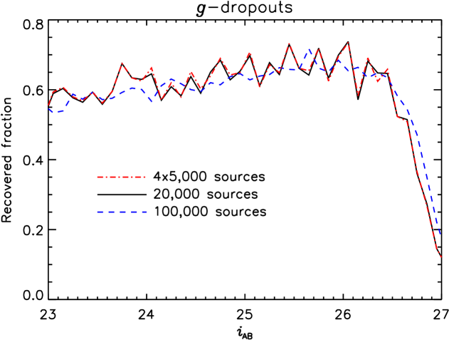
Figure 5: The recovered fraction of injected sources that also satisfy the $g$-dropout criteria, as a function of $i$-band magnitude, for 1 redshift step. Three curves are given for different amounts of injected sources, to see whether, and how, the presence of these sources influences the photometry of the analysis.

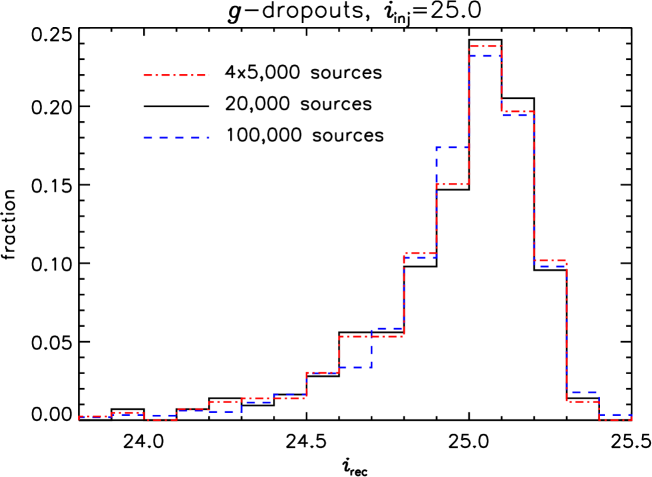
Figure 6: The distribution of measured source magnitudes for a population of injected simulated sources with intrinsic $i$-band magnitude=25.0, for 1 redshift step. Three curves are given for different amounts of injected sources, to see whether, and how, the presence of these sources influences the photometry of the analysis.

The clustering of LBGs is not taken into account. We assume this effect to be insignificant for estimating completeness, as the correlation length, which is typically around 5 Mpc (Hildebrandt et al. 2009), is very small compared to the survey volume. Therefore we spread our simulated sources uniformly over the images.

3.4 Effective volumes

Next we define the function $p(m,z)$ to be the number of sources recovered with an observed magnitude in the interval $[m;m+\Delta m]$, and are selected as dropouts, divided by the number of injected sources with an intrinsic magnitude in the same interval $[m;m+\Delta m]$ and a redshift in the interval $[z;z+\Delta z]$. Note that the definition of $p(m,z)$ is slightly different compared to the one used in e.g. Sawicki & Thompson (2006), as they do not take Eddington bias into account. In our definition, $p(m,z)$ could potentially be $>$ 1 as a result of this bias correction.

The effective volumes ($V_{\rm{eff}}$) of our survey are given by

$$V_{\rm{eff}}(m)=A_{f}\int\frac{dV_{\rm{C}}}{dz}p(m,z)dz,$$ (5)

where $A_{f}$ is the field area in square arcminutes, and $\frac{dV_{\rm{C}}}{dz}$ is the comoving volume per square arcminute, which depends on the adopted cosmology.

The magnitude is measured in the $r$-, $i$-, and $z$-bands for the $u$-, $g$-, and $r$-dropout samples, respectively. These bands probe flux at approximately 1600$\rm{\AA}$ rest-frame of the sources at the expected mean redshifts, so that only a minor k-correction will be sufficient to compare the results for the different epochs directly, see the upper panel of Fig. 7. We transform the apparent magnitudes to absolute magnitudes and perform a k-correction to a rest-frame wavelength of 1600$\rm{\AA}$ using the mean redshifts for each of the dropout samples, i.e. we assume all sources to be at the same redshift.

The uncertainties in the mean redshifts are expected to be approximately $0.1$ for the three dropout samples, as argued in Sect. 2.3. This leads to uncertainties in both distance modulus and k-correction, resulting in a systematic error in the absolute magnitudes of our estimated LF, see the lower panel of Fig. 7. The final uncertainties are about 0.07, 0.05 and 0.04 in the absolute magnitude for the $u$-, $g$-, and $r$-dropout samples, respectively.

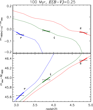
Figure 7: Upper panel: k-correction to 1600$\rm{\AA}$ for the MegaCam $riz$ filters, as a function of redshift based on the 100 Myr old continuously star-forming template with a dust attenuation of $E(B-V)$=0.25. The average redshifts from the simulations and their uncertainties are represented by horizontal error bars. This leads to a corresponding error in the k-correction. Lower panel: Shifts from apparent magnitudes in the MegaCam $riz$ filters, to absolute magnitudes at 1600$\rm{\AA}$. The Distance Modulus and k-correction are taken into account. The uncertainties in the average redshifts of the samples lead to uncertainties in the absolute magnitudes.

4 Results

4.1 The UV Luminosity Function at $z$=3-5

After dividing the number counts by $V_{\rm{eff}}$, which corrects for incompleteness and Eddington bias, and subtracting the distance modulus and the k-correction from the apparent magnitudes, we obtain the LF in absolute magnitudes at 1600$\AA$.

Results from the four fields are binned to $\Delta$mag=0.3, combined, and shown in Fig. 8 and Table 1. Uncertainties in the magnitude direction are due to uncertainties in the redshift distribution of source galaxies. The four independent analyses of the fields allow us to estimate field-to-field variations for each of the data points. Vertical error bars reflect either this uncertainty, or the Poisson noise term, whichever is largest. Usually the field-to-field variance dominates. As a consequence of the way these are computed, Poisson noise is always taken into account.

Table 1: The estimated LFs from the CFHTLS Deep.

	$u$-dropouts	$g$-dropouts	$r$-dropouts
	$\phi_{k}\,[10^{-3}$	$\phi_{k}\,[10^{-3}$	$\phi_{k}\,[10^{-3}$
$M_{\rm{1600,AB}}$	$\rm{Mpc^{-3}\,mag^{-1}}]$	$\rm{Mpc^{-3}\,mag^{-1}}]$	$\rm{Mpc^{-3}\,mag^{-1}}]$
-23.20	0.001 $\pm$ 0.001	-	-
-22.90	0.001 $\pm$ 0.001	-	-
-22.60	0.007 $\pm$ 0.002	0.004 $\pm$ 0.002	0.002 $\pm$ 0.002
-22.30	0.022 $\pm$ 0.007	0.016 $\pm$ 0.003	0.010 $\pm$ 0.002
-22.00	0.057 $\pm$ 0.020	0.035 $\pm$ 0.005	0.032 $\pm$ 0.010
-21.70	0.113 $\pm$ 0.028	0.086 $\pm$ 0.010	0.065 $\pm$ 0.015
-21.40	0.254 $\pm$ 0.027	0.160 $\pm$ 0.027	0.121 $\pm$ 0.016
-21.10	0.497 $\pm$ 0.061	0.287 $\pm$ 0.060	0.234 $\pm$ 0.028
-20.80	0.788 $\pm$ 0.110	0.509 $\pm$ 0.061	0.348 $\pm$ 0.025
-20.50	1.188 $\pm$ 0.267	0.728 $\pm$ 0.067	0.494 $\pm$ 0.050
-20.20	1.745 $\pm$ 0.377	1.006 $\pm$ 0.040	0.708 $\pm$ 0.030
-19.90	2.240 $\pm$ 0.373	1.465 $\pm$ 0.147	1.123 $\pm$ 0.211
-19.60	2.799 $\pm$ 0.519	1.756 $\pm$ 0.063	1.426 $\pm$ 0.229
-19.30	3.734 $\pm$ 0.863	2.230 $\pm$ 0.305	1.624 $\pm$ 0.095
-19.00	4.720 $\pm$ 0.866	2.499 $\pm$ 0.564	1.819 $\pm$ 0.630
-18.70	3.252 $\pm$ 1.508	3.038 $\pm$ 0.370	-

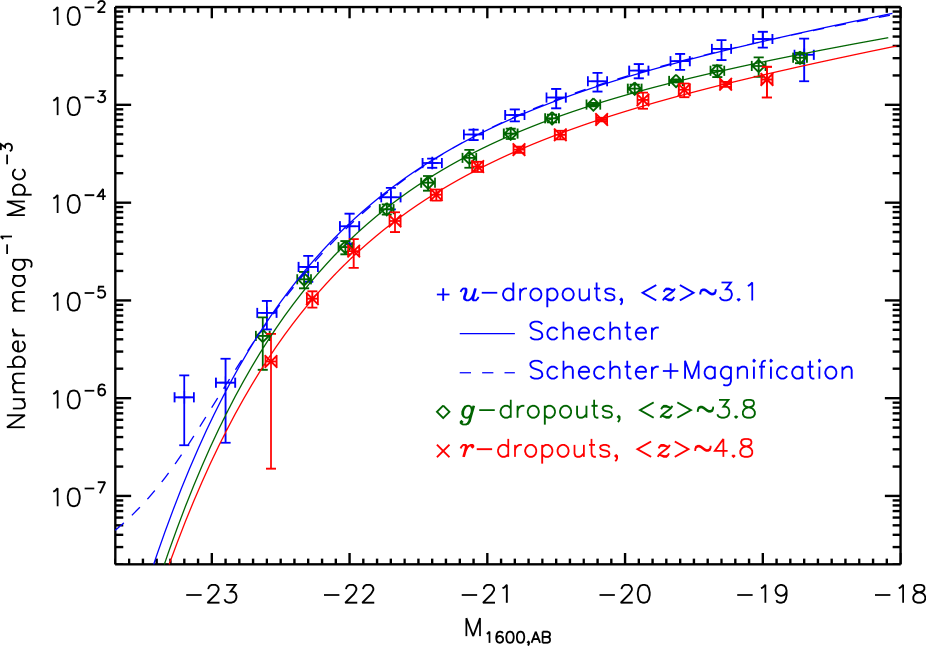
Figure 8: The LFs of LBGs in the CFHTLS-Deep fields. Data points and best-fitting Schechter functions are shown for the $u$(blue)-, $g$(green)-, and $r$(red)-dropouts. For legibility we applied a small offset on the x-axis values of the $g$-, and $r$- dropouts. The dashed blue curve shows the best fitting Schechter function for the $u$-dropouts after magnification effects have been included, as described in Sect. 4.1.1.

We fit a Schechter function (Schechter 1976) to the binned data points,

$$\phi(M)dM=0.4\ln(10)\phi^{*}10^{0.4(\alpha+1)(M^{*}-M)}\exp(-10^{0.4(M^{*}-M)}),$$ (6)

with $M^{*}$ being the characteristic magnitude, $\alpha$ being the faint-end slope, and $\phi^{*}$ being the overall normalisation.

Using $\chi^{2}$ statistics on a three dimensional grid of $500^{3}$ different Schechter parameter combinations, we find the minimal value ($\chi_{\rm{min}}^{2}$) for each of the dropout samples yielding the best fit values. To estimate the errors in the fitted parameters, we project the 3-dimensional distribution of $\chi^{2}$ to 3 planes by taking the minimum $\chi^{2}$ along the projected dimension. In Fig. 9 the 68.3% and 95.4% confidence levels are shown, which correspond to a $\Delta\chi^{2}$=2.3 and 6.17 with respect to $\chi^{2}_{\rm min}$. In Table 2 we give the 68.3% confidence levels on each individual parameter, corresponding to $\Delta\chi^{2}$=1.0.

Note, however, that this error estimate assumes Gaussian errors, and that the errors on the data points are independent. Especially for the $u$-dropouts this is probably not the case. The normalisation of the LF seems to be systematically slightly different for each of the fields (see also Fig. 1), giving a systematic uncertainty in $\phi^{*}$ of about 30%. For the $u$-dropouts this effect is largest because of a slightly more uncertain flux calibration in the $u$-band compared to the $g$- and $r$-bands. The effective filter throughput changes with time in the UV as the atmosphere is changing, and also the camera is less sensitive in this wavelength regime resulting in larger shot-noise.

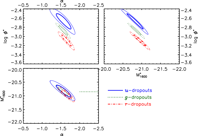
Figure 9: The 68% and 95% likelihood contours for different Schechter parameter combinations. Shown are the results for the $u$-dropouts at $z\sim 3$ (blue, solid), the $g$-dropouts at $z\sim 4$ (green, dots), and the $r$-dropouts at $z\sim 5$ (red, dash-dots). The $u$-dropout contours represent the best Schechter parameters when we include magnification effects, as described in Sect. 4.1.1.

Table 2: A comparison between the best fitting Schechter parameters and their 68% confidence intervals for the $u$-, $g$-, and $r$-dropouts.

		$\phi^{*}$
Sample	$\rm{M}_{\rm{UV}}^{*}$ a	[$10^{-3}\,\rm{Mpc}^{-3}$]	$\alpha$	$\chi^{2}/\rm{dof}$
$u$	$-20.94^{+0.14}_{-0.13}$	$1.79^{+0.51}_{-0.38}$	$-1.65^{+0.12}_{-0.11}$	$0.52$
$g$	$-20.84^{+0.09}_{-0.09}$	$1.36^{+0.23}_{-0.20}$	$-1.56^{+0.08}_{-0.08}$	$0.36$
$r$	$-20.94^{+0.10}_{-0.11}$	$0.83^{+0.15}_{-0.14}$	$-1.65^{+0.09}_{-0.08}$	$0.19$
$u^{\mathrm{b}}$	$-20.84^{+0.15}_{-0.13}$	$2.11^{+0.63}_{-0.45}$	$-1.60^{+0.14}_{-0.11}$	$0.41$

• Due to uncertainties in the redshift distributions there is an additional error component of 0.07, 0.05, and 0.04 in the estimated $\rm{M}_{\rm{UV}}^{*}$ for the $u$-, $g$-, and $r$-dropout samples, respectively.

• Best-fitted Schechter parameters for a model where the function is modified with a magnification distribution.

4.1.1 Magnification contribution at low densities

Due to inhomogeneities in the matter distribution between distant sources and the observer, paths of photons get slightly perturbed. This results in a distortion of the shape and a magnification of distant sources. When a source is magnified by a factor $\mu$, the flux gets boosted by the same amount. One can relate an intrinsic luminosity distribution to an observed distribution if the magnification distribution is known, as was shown by Jain & Lima (2010). Hilbert et al. (2007) estimate magnification distributions for different source redshifts by shooting random rays through a series of lens planes created from the Millennium Simulation. The width of the magnification distribution is found to increase with increasing source redshift, and the peak position of the distribution decreases slightly with increasing source redshift.

Magnification can account for a strong deviation from a Schechter function where the slope of the intrinsic luminosity distribution is very steep, see Jain & Lima (2010). We stress again that we measure the LF from a volume that is much larger than has been used before. The bright end of our $g$-, and $r$-dropout samples suffers from increasing amounts of contamination. Only for the $u$-dropouts we probe the distribution of $u$-dropouts at the bright end down to a density of $10^{-6}\,\rm{mag}^{-1}\,\rm{Mpc}^{-3}$. We use the magnification distribution for a source redshift of $z=3.1$ that was kindly provided by Stefan Hilbert to improve our model to the data.

Writing the LF as a function of magnitude, we use the following equation to correct the Schechter function for magnification effects. It is equivalent to the expression used by Jain & Lima (2010).

$$\phi(m_{obs})=\int d\mu\,P(\mu)\,\phi^{*}(m_{obs}+2.5\log(\mu)),$$ (7)

where $\phi^{*}$ is the Schechter function defined by Eq. 6. The new function yields a slightly better fit to the bright end of the LF, reducing the formal $\chi^{2}/\rm{dof}$ from 0.52 to 0.41. Find the new Schechter parameters, together with their 68.3% confidence levels in Table 2, and their 2-dimensional 68.3% and 95.4% confidence contours plotted in Fig. 9. The best fitting function is the dashed curve in Fig. 8.

As the bright selected $u$-dropouts are likely to be significantly magnified, we expect them to appear close to a massive foreground galaxy or group of galaxies that acts as a lens. We inspected the brightest ($r_{AB}<$23.2) $u$-dropouts by eye and find that this is indeed the case for many of them. Note that the model is still uncertain as the Millennium simulation does not include baryonic matter, and assumes $\sigma_{8}=0.9$ (Springel et al. 2005), where recent estimates indicate a lower value around 0.8 (Komatsu et al. 2010). Also, in the magnification probability distribution the possibility of multiply imaged systems is ignored. To rule out contamination in the LBG sample at the bright end of the LF, the nature of each bright object has to be verified spectroscopically.

A statistically much better sample can be selected from the CFHT Legacy Survey Wide, consisting of 170 square degree imaging in $ugriz$ of shallower depth. We leave this for future studies.

4.2 The UV Luminosity Density and SFR Density

Next we estimate the UV luminosity density (UVLD) at the different epochs. To be able to compare our results with the results from previous studies, we will integrate the data points down to $L=0.3L^{*}_{z=3}$, where $L^{*}_{z=3}$ $(\rm{=9.4\times 10^{28}\,erg\,s^{-1}\,Hz^{-1}\,at\,1600\AA})$ is the characteristic luminosity of our $u$-dropout sample. Results are shown in the odd-numbered rows of Col. 3 in Table 3. However, for steep faint-end slopes of $\alpha<-1.6$, more than 50% of the UV luminosity is expected to be emitted by lower luminosity sources. Therefore we will make a second estimate of the UV luminosity density by integrating the best-fitting Schechter function over all luminosities. This results in

$$\rho_{\rm{UV}}=\phi^{*}L^{*}\Gamma(\alpha+2),$$ (8)

where $\Gamma$ is Euler’s Gamma function. Although this full integral of the LF depends strongly on uncertainties in the faint-end slope, we use it to provide an upper limit to the UVLD. The results are shown in the even-numbered rows of Col. 3 in Table 3.

The effective extinction in the UV is a strong function of the amount of dust. At these high redshifts ($z\gtrsim 3$) the only estimate for the amount of dust is based on a measure of the UV continuum slope. Note however that there is a strong degeneracy between the age and the amount of dust in the template if the rest-frame IR is not covered, see e.g. Papovich et al. (2001).

Bouwens et al. (2009) recently measured the UV-continuum slope of LBGs at high redshifts from deep HST data, from which the amount of dust obscuration could be estimated as a function of LBG magnitude. The values they find at the characteristic magnitudes of our samples are $E(B-V)=0.15$ for $z=3,4$, and $E(B-V)=0.10$ for the $z\sim 5$ sample. Bouwens et al. (2009) find a decreasing amount of dust for fainter magnitudes. For consistency we will use the relationships they estimate to correct for dust extinction in our data, and not the values from Sect. 3.1.

Meurer et al. (1999) find a relation between the UV-continuum slope and the extinction by dust. Bouwens et al. (2009) use this relation and find, upon integrating down to $L=0.3L^{*}_{z=3}$, density correction factors of $6.0^{+1.8+2.1}_{-1.4-1.6}$, $5.8^{+0.8+2.1}_{-0.7-1.5}$, and $2.7^{+0.7+1.0}_{-0.5-0.7}$ for the three redshift samples, respectively. Both random errors and systematic errors are quoted (Bouwens et al. 2009).

We now convert the UV luminosity density into the star formation rate density, $\rho_{\rm{SFR}}$, at the different epochs using (Madau et al. 1998),

$$L_{UV}=8.0\times 10^{27}\,\left(\frac{\rm{SFR}}{M_{\sun}\rm{yr^{-1}}}\right)\,\rm{erg\,s^{-1}\,Hz^{-1}}.$$ (9)

This relation assumes a 0.1-125$\rm{M}_{\sun}$ Salpeter IMF and a constant star formation rate of $\gtrsim$ 100 Myr. The resulting estimates of $\rho_{\rm{SFR}}$ are shown in Col. 4 of Table 3, where we have corrected for dust extinction. In Sect. 5.4 we compare these estimates to values reported in previous studies.

Table 3: The $\rho_{\rm{UV}}$ and $\rho_{\rm{SFR}}$ for the different dropout samples. The first lines for each sample correspond to sums over the data points down to $L=0.3L^{*}_{z=3}$ while the second lines correspond to integrals over the best-fit Schechter functions.

Sample	Integral limit	$\rho_{\rm{UV}}$ $[10^{26}$	$\rho_{\rm{SFR}}$
		$\rm{erg\,s^{-1}\,Hz^{-1}\,Mpc^{-3}}]^{\mathrm{a}}$	$[\rm{M_{\sun}\,yr^{-1}\,Mpc^{-3}}]^{\mathrm{a,b}}$
$u$	$L>0.3L^{*}_{z=3}$	$1.73\pm 0.09$	$0.129^{+0.064}_{-0.036}$
	Schechter	$4.41$	0.154
$g$	$L>0.3L^{*}_{z=3}$	$1.07\pm 0.03$	$0.078^{+0.032}_{-0.019}$
	Schechter	$2.62$	0.092
$r$	$L>0.3L^{*}_{z=3}$	$0.80\pm 0.03$	$0.027^{+0.013}_{-0.007}$
	Schechter	$2.19$	0.038

• Due to uncertainties in the redshift distributions, there is an additional error component of $\sim$7%, $\sim$5%, and $\sim$4% in the estimated $\rho_{\rm{UV}}$ and $\rho_{\rm{SFR}}$ values for the $u$-, $g$-, and $r$-dropout samples, respectively.

• Corrected for dust extinction using the luminosity dependent correction factors from Bouwens et al. (2009). Systematic errors as a result from the age-dust degeneracy are also included.

Note, however, that some sources like AGN, which might be included in our dropout samples, add to the total UV luminosity density in the Universe, though do not contribute to the SFRD.

4.3 Robustness of our results

Our fiducial template model is a 100 Myr old continuously star-forming galaxy with a uniform distribution of dust centred around $E(B-V)$=0.25. This dust distribution was chosen such that the distribution of UV-continuum slopes of the recovered simulated sources matches the distribution of UV-continuum slopes in the real data (see Fig. 3). We test some of the assumptions we made in Sect. 3.1 by checking their influence on the final LFs.

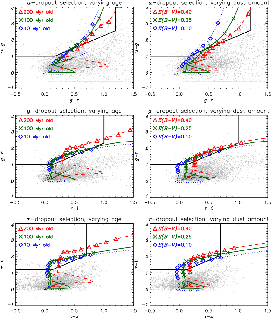
Figure 10: The grey points represent the colours of 10,000 objects in field 1 of the CFHTLS Deep. The black boxes are defined by Eqs. 1-3 and are used to select $u$-(top panels), $g$-(middle panels), and $r$-(bottom panels) dropouts. The coloured tracks represent the colours of a template galaxy as a function of $z$. They are evaluated at intervals of $\Delta z$=0.1. The symbols mark redshifts from 2.5 to 3.5, from 3.2 to 4.2 and from 4.2 to 5.2 for $u$-, $g$-, and $r$-dropouts respectively. The green curve with $\times$-symbols represents a reference model, a 100 Myr old continuously star-forming template with a dust attenuation of $E(B-V)$=0.25. In the left panels we consider redder (bluer) templates by increasing (decreasing) the template age, see the red (blue) curves and the $\triangle$ ($\Diamond$)-symbols. In the right panels we consider redder (bluer) templates by increasing (decreasing) the amount of dust in the template, see the red (blue) curves and the $\triangle$ ($\Diamond$)-symbols. Note that we use a distribution of dust in our fiducial analysis (see Sect. 3.1).

As a reference SED we use a 100 Myr old galaxy model with constant star formation and a single dust attenuation value of $E(B-V)$=0.25. We consider redder (bluer) templates by either increasing (decreasing) the age of the star-forming period, or increasing (decreasing) the amount of dust. In Fig. 10 the colours of these alternative templates, as they would be measured by the MegaCam $ugriz$ filter set, are shown as a function of redshift. As the quality of the Schechter fit is high in all cases ($\chi^{2}/\rm{dof}<1.0$), we present the differences by comparing the Schechter parameters:

• The faint-end slope $\alpha$ depends on the colour of the spectral template. In the $g$-, and $r$-dropout samples, redder templates tend to give steeper $\alpha$ than bluer templates. The reason for this is as follows, with the $g$-dropouts as an example. Sources in the selection box have red observed $g-i$ colours. For faint magnitudes (note that the reference magnitude is measured in the $i$-band), the $g$-band magnitude exceeds the limiting magnitude of the survey. Only a lower limit on $g-r$ can then be given and the source moves out of the dropout selection box. The magnitude at which this happens depends on the $g-i$ colour of the template. As the average $g-i$ colour in the selection box is redder for red templates (Fig. 10), the detection rate of red sources is suppressed at faint magnitudes. This argument holds for any red template in the $g$-, and $r$-dropout samples. Fig. 10 indicates that the opposite effect happens in the $u$-dropout sample as the $u-r$ colour is generally bluer (redder) for redder (bluer) templates in the selection box. This effect is indeed also inferred from the simulations. There is an additional effect due to the requirement that $g$-dropouts are not detected in $u$, and that $r$-dropouts are neither detected in $g$ nor in $u$. This suppresses the detection of bright $g$-, and $r$-dropouts, especially at low redshifts. The bluer the $u-i$ colour for the $g$-dropouts (i.e. the bluer the template), the stronger this effect is. A similar argument holds for the $r$-dropouts. Therefore the $V_{\rm{eff}}$’s are higher in the faint magnitude regime, so that the LFs are lower at this end. The ranges of best-fitted $\alpha$ values, for the template spectra we considered, are $-1.82<\alpha<-1.38$ for the $u$-, $-1.82<\alpha<-1.42$ for the $g$-, and $-2.14<\alpha<-1.40$ for the $r$-dropout sample.

• The characteristic magnitude, $M^{*}$, does not sensitively depend on the template spectrum chosen. The ranges of best-fitted $M^{*}$ values, for the template spectra we considered, are $-20.88<M^{*}<-20.72$ for the $u$-, $-21.06<M^{*}<-20.74$ for the $g$-, and $-21.26<M^{*}<-20.88$ for the $r$-dropout sample. However, another systematic uncertainty in this parameter is due to the unknown redshift distribution of source galaxies, see Fig. 7, which depends on the mix of templates used by Hildebrandt et al. (2009).

• The normalisation $\phi^{*}$ decreases (increases) when the faint-end slope becomes steeper (shallower). The best-fit Schechter parameters move then in the direction of the degeneracy of the ellipse in the upper left part of Fig. 9. The ranges of best-fitted $\phi^{*}$ values [$10^{-3}\,\rm{Mpc}^{-3}$], for the template spectra we considered, are $1.36<\phi^{*}<2.89$ for the $u$-, $0.76<\phi^{*}<1.74$ for the $g$-, and $0.39<\phi^{*}<1.12$ for the $r$-dropout sample.

Some studies (e.g. Sawicki & Thompson 2006) make use of a starburst template instead of a continuously star-forming model. The stellar population in a starburst template is older on average, and therefore the colours will be redder. However, for a template age of 100 Myr the difference in colours is very small. We compare the Schechter parameters that we measure after using our reference model (i.e. a 100 Myr continuously star-forming template with a dust reddening of $E(B-V)$=0.25) with a model where we change the star-formation law to a starburst. We find the Schechter parameters to change in the directions that are expected for a redder template, as explained above. However the differences are insignificant since they are much smaller than the statistical errors on the Schechter parameters.

We stress again that we use a mix of dust amounts in our standard analysis to match the UV-continuum slope distribution that is measured from the data. Especially for the $u$-, and $g$-dropouts this puts strong constraints on the combination of the age and the amount of dust in the model template, so that we can reduce the systematic error to a minimum.

To justify the assumptions we make regarding the shapes of our simulated sources we also estimated the systematic error on the LF due to this component. Because we expect similar results in the three dropout samples, we only run these simulations for the $g$-dropouts. We inject sources that are 0.05” larger than the measured position-dependent PSF, and compare values of Moffat parameter $\beta=3.0$ and $\beta=5.0$ with our fiducial $\beta=4.0$ parameter. We find the following:

• As expected, $\alpha$ becomes steeper for more extended sources (i.e. increasing the $R_{0}$ or decreasing $\beta$), as this causes the peak surface brightness to drop. This only significantly affects the $V_{\rm{eff}}$’s at the faint end of the LF. Estimations of $\alpha$ range from $-1.94<\alpha<-1.36$. A similar change is expected for the $u$-, and $r$- dropout studies. The other Schechter parameters, $\phi^{*}$ and $M^{*}$, then also change slightly as they move in the direction of the degeneracy in Fig. 9.

Furthermore we find that, based on the different template spectra, the estimated UV luminosity density varies. The ranges are, upon integration down to $L<0.3L^{*}_{z=3}$, in units $\rm{[10^{26}erg\,s^{-1}\,Hz^{-1}\,Mpc^{-3}}]$, $1.30<\rho_{\rm{UV}}<1.98$ for the $u$-, $0.92<\rho_{\rm{UV}}<1.15$ for the $g$-, and $0.80<\rho_{\rm{UV}}<0.92$ for the $r$-dropouts.

In order to illustrate the effect that the Eddington bias can have on LF estimations we repeat our analysis with slightly changed $p(m,z)$. In the completeness simulations we bin the recovered sources by their intrinsic magnitude instead of their recovered magnitude. Doing so leaves the Eddington bias uncorrected. We find that the Schechter fit to the resulting LFs are not as good as for our standard analysis, especially for the $g$-, and $r$-dropouts, where we find that $\chi_{\rm{min}}^{2}/\rm{dof}$ would be 1.0 and 3.0, respectively. For the $u$-dropouts the best-fitting parameters are not changed significantly, but for the $g$-, and $r$-dropouts the faint-end slope steepens while the normalisation of the Schechter function decreases.

Note that we did not account for the presence of Lyman- $\alpha$ emission in our simulations, although this line clearly contributes to broadband fluxes. Shapley et al. (2003) measured the contribution of this line in the spectra of $z\sim 3$ LBGs and concluded that only $\sim 25\%$ of the sample showed significant Ly $\alpha$ emission such that EW(Ly$\alpha$) $>20\AA$, see also Reddy et al. (2008). Although the relative contribution of this line is thought to increase towards higher redshift and fainter continuum luminosity, this has not been quantified yet. We will therefore describe possible biasses due to the presence of this line in the measurement of the LF only qualitatively.

If the line appears in emission, it contributes to the flux in the CFHT $g$-band for redshifts of about $2.5<z<3.5$, in the $r$-band for redshifts of about $3.7<z<4.6$, in the $i$-band for redshifts of about $4.8<z<5.9$, and in the $z$-band for redshifts of about $z>5.8$. Following the redshift distributions from Hildebrandt et al. (2009), we expect that the line predominantly contributes to the middle band in a two colour selection for the $u$-, and $r$- dropout samples, moving the source to the upper left in Fig. 10. This effect causes the effective volumes to rise, thereby lowering the LF measurement. If the line indeed gets stronger at faint magnitudes, this would bias the LF measurement and results in a shallower alpha. In our $g$-dropout sample the line is expected to contribute to the flux in both the $r$- and $i$-band, depending on the redshift of the particular source. In the case where the line falls in the $r$-band, the effective volumes rise and the LF we measured is too high. For the redshifts where the line falls in the $i$-band, the sources would move to the right in Fig. 10 so that the effective volumes are decreased and the LF increases. To estimate which effect prevails, the redshift distribution needs to be measured spectroscopically. Some objects show Ly-$\alpha$ in absorption rather than emission, which would give the opposite effect.

Note that Bouwens et al. (2007) model the contribution of Ly$\alpha$ in the measurement of their LF, by using a simple model where 33% of the $z\sim 4-5$ LBGs have EW(Ly $\alpha$ )= 50 $\AA$, independent of the continuum luminosity. They find that this affects the normalisation of the LF by only $\sim 10\%$. However, we stress again that the measure of $\alpha$ might be biased if the strength of the line depends on the continuum luminosity.

4.4 The evolving galaxy population

Although we can measure the UV luminosity density with great accuracy, an estimate of the SFR Density depends sensitively on the dust extinction correction. Using the prescription from Bouwens et al. (2009), we find that the SFR Density shows a significant increase by a factor of 4-5 between $z\sim 5$ and $z\sim 3$ .

We find a strong increase in $\phi^{*}$ between $z\sim 5$ and $z\sim 3$ by a factor of 2.5, which is a robust result. The characteristic magnitude, $M_{\rm{UV}}^{*}$, however is not very well constrained by our data set. This is due to uncertainties in the redshift distributions of the source galaxies, as there are no spectroscopic data available. Our data are consistent with a non-evolving $M_{\rm{UV}}^{*}$ ($\sim-20.9$) between $z\sim 5$ and $z\sim 3$. Our data do not show an evolution of the faint-end slope, and indicate $\alpha\sim-1.6$ in this epoch.

5 Comparison with previous determinations

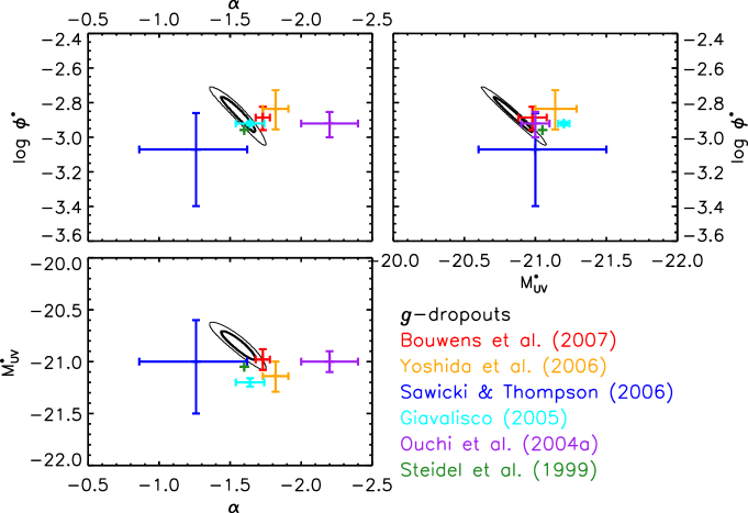
Figure 12: Similar as Fig. 11, but now a comparison at $z\sim 4$.

Before we compare our results from each of the samples with Schechter parameters reported from previous determinations in the literature, there are a few things that should be noted. We will compare results at redshifts of $around$ 3, 4 and 5. The LBGs are generally selected from different surveys and filter sets, and therefore intrinsically slightly different galaxies may be selected, studied and compared. Also the rest-frame wavelength at which the LF is estimated, varies. We compared the LFs at 1600$\rm{\AA}$, while e.g. Sawicki & Thompson (2006) measured the LF at 1700$\rm{\AA}$, and e.g. Giavalisco et al. (2004) did their analysis at 1500$\rm{\AA}$. Some of the studies described below make use of identical or partially overlapping datasets. Our analysis, on the contrary, is completely independent from previous determinations, except for the dust extinction correction in our SFR density estimate. Furthermore the errors of several other studies could be underestimated because only the Poisson noise component is taken into account, as other noise components (e.g. cosmic variance) are difficult to estimate with the typical small survey volumes of other surveys. Also note that we compare our 2-dimensional error ellipses with 1-dimensional error bars that were attained after marginalizing over the two other Schechter parameters. This dilutes information on degeneracies between Schechter parameters. For these reasons the comparisons in this section will be rather qualitative, and are meant to put our results into context. Comparisons of the Schechter parameters are shown in Table 4, and in Figs. 11, 12 & 13, and will be discussed below.

Table 4: Our estimated Schechter parameters compared with values reported in the literature, for the three dropout samples.

Reference	$M_{UV}^{*}$	$\phi^{*}$	$\alpha$
		[$10^{-3}\,\rm{Mpc}^{-3}$]
$u$-dropouts
This work, Schechter	$-20.94^{+0.14}_{-0.13}$	$1.79^{+0.51}_{-0.38}$	$-1.65^{+0.12}_{-0.11}$
This work, Schechter+Magnification	$-20.84^{+0.15}_{-0.13}$	$2.11^{+0.63}_{-0.45}$	$-1.60^{+0.14}_{-0.11}$
Reddy & Steidel (2009)	$-20.97\pm 0.14$	$1.71\pm 0.53$	$-1.73\pm 0.13$
Sawicki & Thompson (2006)	$-20.90^{+0.22}_{-0.14}$	$1.70^{+0.59}_{-0.32}$	$-1.43^{+0.17}_{-0.09}$
Arnouts et al. (2005)	$-21.08\pm 0.45$	$1.62\pm 0.90$	$-1.47\pm 0.21$
Poli et al. (2001)	$-20.84\pm 0.37$	$2.3$	$-1.37\pm 0.19$
Steidel et al. (1999)	$-21.04\pm 0.15$	$1.4$	$-1.60\pm 0.13$
$g$-dropouts
This work	$-20.84\pm 0.09$	$1.36^{+0.23}_{-0.20}$	$-1.56\pm 0.08$
Bouwens et al. (2007)	$-20.98\pm 0.10$	$1.3\pm 0.2$	$-1.73\pm 0.05$
Yoshida et al. (2006)	$-21.14^{+0.14}_{-0.15}$	$1.46^{+0.41}_{-0.35}$	$-1.82\pm 0.09$
Sawicki & Thompson (2006)	$-21.0^{+0.4}_{-0.5}$	$0.85^{+0.53}_{-0.45}$	$-1.26^{+0.40}_{-0.36}$
Giavalisco (2005)	$-21.20\pm 0.04$	$1.20\pm 0.03$	$-1.64\pm 0.10$
Ouchi et al. (2004a)	$-21.0\pm 0.1$	$1.2\pm 0.2$	$-2.2\pm 0.2$
Steidel et al. (1999)	$-21.05$	$1.1$	$-1.6$ (fixed)
$r$-dropouts
This work	$-20.94^{+0.10}_{-0.11}$	$0.83^{+0.15}_{-0.14}$	$-1.65^{+0.09}_{-0.08}$
Bouwens et al. (2007)	$-20.64\pm 0.13$	$1.0\pm 0.3$	$-1.66\pm 0.09$
Oesch et al. (2007)	$-20.78\pm 0.16$	$0.9\pm 0.3$	$-1.54\pm 0.10$
Iwata et al. (2007)	$-21.28\pm 0.38$	$0.41^{+0.29}_{-0.30}$	$-1.48^{+0.38}_{-0.32}$
Yoshida et al. (2006)	$-20.72^{+0.16}_{-0.14}$	$1.23^{+0.44}_{-0.27}$	$-1.82$ (fixed)
Giavalisco (2005)	$-21.06\pm 0.05$	$0.83\pm 0.03$	$-1.51\pm 0.18$
Ouchi et al. (2004a)	$-20.3\pm 0.2$	$2.4\pm 1.0$	$-1.6$ (fixed)

5.1 Comparison at $z$=3

We compare the results from our $u$-dropout sample with several Schechter parameters reported in the literature. Sawicki & Thompson (2006) estimated the LF from the Keck deep fields, from $U_{n}GR$-selected star-forming galaxies. Their survey area is about 60 times smaller than the CFHTLS-Deep. The depth of their observations is slightly deeper than ours, but due to our Eddington bias correction, we are able to probe the LFs down to similar magnitudes. Reddy & Steidel (2009) estimate a LF at $z\sim 3$, from 31 spatially independent fields, having a total area of about a quarter of ours. Their sample contains several thousands of spectroscopic redshifts at $z$=2-3. Arnouts et al. (2005) mainly focussed on the galaxy LF at lower redshifts ($0.2\leq z\leq 1.2$) from $GALEX$-data, but their redshift range was extended using 173 galaxies at $z\sim 3$ from the HDF sample. Poli et al. (2001) used the HDF-N, HDF-S and NTT-DF samples to estimate the LF in the range $2.5\la z\la 3.5$. Their sample was therefore selected from a very small volume, which makes their results susceptible to cosmic variance. Steidel et al. (1999) pioneered this work, and estimated the UV LF from 0.23 deg² of moderately deep data. Their study was supported by a spectroscopic redshift sample. This data is included in the study by Reddy & Steidel (2009).

Our results agree within the $1-\sigma$ level with the results from previous determinations at $z\sim 3$. Note that the other data points lie in the direction of the elongated ellipse, and therefore in the direction of the degeneracy we find.

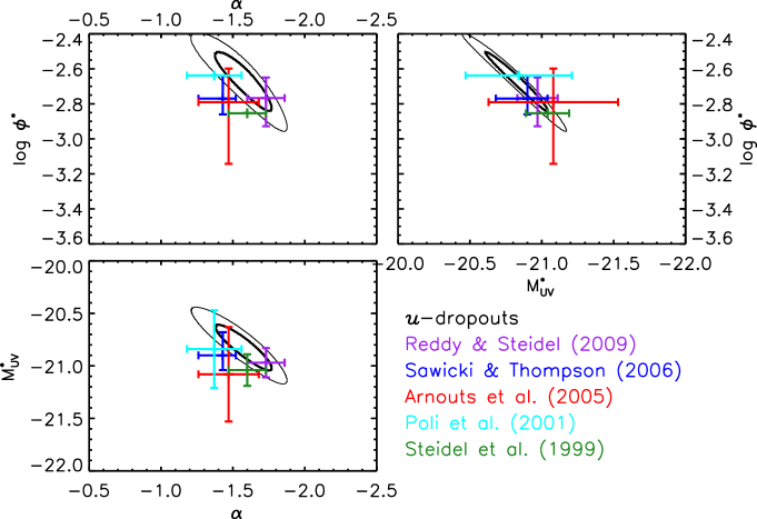
Figure 11: Comparison at $z\sim 3$. The ellipses represent the 68% and 95% confidence contours for different Schechter parameter combinations, based on our study. The error bars reflect the 68% confidence limits on the results from previous studies. Our results agree within the 1-$\sigma$ level with most of the other determinations.

5.2 Comparison at $z$=4

Our $g$-dropout sample is compared with the $z\sim 4$ sample from Sawicki & Thompson (2006), selected from the $GRI$ filter sets on the Keck telescope. Their area is identical to the one from which the $z\sim 3$ LF was estimated. Steidel et al. (1999) also estimated the $z\sim 4$ LF with a similar filter set as Sawicki & Thompson (2006), but did not probe deep enough to be able to constrain the faint-end slope $\alpha$. This parameter was set equal to the value found at $z=3$, namely $\alpha=-1.6$. Yoshida et al. (2006) presented the LF for 3808 $BRi$’-selected LBGs, selected from the Subaru Deep Field project. Ouchi et al. (2004a) selected a $z\sim 4$ LBG sample from Subaru imaging, supported by a sample of 85 spectroscopically identified objects. Giavalisco et al. (2004) used a $\sim$0.09 deg² sample from the GOODS to estimate a LF for $B_{450}V_{606}z_{850}$-selected LBGs. Bouwens et al. (2007) used the deep HST ACS fields, including the HUDF and the GOODS, to select a sample of 4671 B-dropouts, from which they estimated the UV LF to $M_{1600,AB}=-16.26$.

With this data set we have been able to measure the Schechter parameters for the $g$-dropout sample with very high statistical accuracy. Note however that several systematic uncertainties, which we comment upon in Sect. 4.3, are not included in our error ellipses. Our results agree within the $1-\sigma$ level with many of the $z\sim 4$ results in the literature. However, there is still some tension in measurements of the faint-end slope $\alpha$. The characteristic magnitude, $\rm{M}_{\rm{UV}}^{*}$, we measure, is slightly fainter than the values we found in the literature.

5.3 Comparison at $z$=5

At $z\sim 5$, Iwata et al. (2007) reported the UV LF from a combination of HDF and Subaru images, totalling a survey area about 1/9 of ours. Oesch et al. (2007) based their study on approximately 100 LBGs from very deep ACS and NICMOS imaging. Yoshida et al. (2006) also defined a $z\sim 5$ sample from their observations, combining $Vi^{\prime}z^{\prime}$ and $Ri^{\prime}z^{\prime}$ selected objects, as did Ouchi et al. (2004a). Giavalisco et al. (2004) selected 275 $V_{606}i_{775}z_{850}$ LBGs to estimate a $z\sim 5$ UV LF. Bouwens et al. (2007) also measured a sample of 1416 V-dropouts from their deep HST ACS sample, which resulted in an estimation of the UV LF down to $M_{1600,AB}=-17.16$.

Similar to the Schechter parameters found for $z\sim 4$, there is a large discrepancy in the literature for the Schechter parameters at $z\sim 5$. The statistical uncertainties in the Schechter parameters is very small for our $r$-dropout sample. Note however that several systematic uncertainties are not included in these error ellipses, see Sect. 4.3. Our results agree reasonably well, within the $1-\sigma$ level, with many previous determinations at $z\sim 5$.

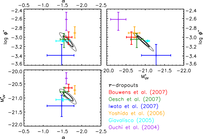
Figure 13: Similar as Fig. 11, but now a comparison at $z\sim 5$.

5.4 Comparison of the SFR density

In Fig. 14 we compare the SFR density values given in Table 3 to values reported by Schiminovich et al. (2005), who made use of low-$z$ GALEX data, Reddy & Steidel (2009) at intermediate $z$, and Bouwens et al. (2009) at high $z$. The uncorrected SFRDs are in good agreement with each other and show a smooth redshift evolution. However, it is clear that the dust correction is the major uncertainty because of the age-dust degeneracy. We use the same dust correction as Bouwens et al. (2009) and also include systematic uncertainties in the error bars.

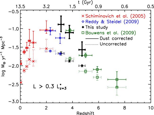
Figure 14: $\rho_{\rm{SFR}}$ as a function of redshift and cosmic time. Dotted: SFRD uncorrected for dust. Solid: the dust corrected SFRD, where we use a luminosity dependent dust correction factor from Bouwens et al. (2009). Note that we included both random and systematic errors in our dust correction, unlike most other studies.

6 Summary & Conclusions

In this paper we use the CFHT Legacy Survey Deep fields to estimate the UV Luminosity Functions of the largest $u$, $g$-, and $r$-dropouts samples to date. As our samples are all extracted from the same dataset this study is ideally suited to study a time evolution of the luminosity function in the redshift regime $z=3-5$. Thanks to the large volumes we probe with our 4 square degree survey, cosmic variance plays a negligible role in our analysis. We are now able to study the bright end of the luminosity function with unprecedented accuracy. Furthermore, given the depth of the stacked MegaCam images, we probe the faint end of the luminosity function with comparable precision as the deepest ground based surveys have done before. This unique combination gives us the opportunity to not only estimate the Schechter parameters for the different luminosity functions, but also to study a possible deviation from this commonly used fit.

In the $u$-, and $g$-dropout samples of our survey we are able to measure the UV continuum slope directly from the data. This allows us to simulate sources that have the same distribution of UV slopes, which is important for an accurate estimate of the Schechter parameters.

We find the faint-end slope $\alpha$ to not evolve significantly in the redshift range we probe, and to have a value of around $-1.6$. This parameter however, is not very strongly constrained by our ground based survey, as this parameter depends on some of the assumptions made.

We do not find a significant evolution in $M_{\rm{UV}}^{*}$, and argue that this might be due to insufficient knowledge of the redshift distribution of the source galaxies. The conversion of apparent to absolute magnitudes depends strongly on these distributions, and an uncertainty in the distance modulus directly propagates into an equal uncertainty in $M_{\rm{UV}}^{*}$. This parameter is therefore poorly constrained by this study, until a more reliable redshift distribution is available.

We find a strong evolution in $\phi^{*}$, which we argue to be significant. The normalisation of the LBG density, $\phi^{*}$, increases by a factor of $\sim 2.5$ from $z\approx 5$ to $z\approx 3$, an increase that cannot be explained by any change in the assumptions tested. We therefore conclude that the UV luminosity density is increasing in the corresponding epoch, in a way that does not strongly differ with magnitude.

The SFR Density does increase significantly, by a factor of $\sim 3$, between $z\sim 5$ and $z\sim 4$. We find a smaller, but less significant increase between $z\sim 4$ and $z\sim 3$.

With our 4 square degree survey we probe densities that are at least four times lower than any of the studies we compared our results to. We find a substantial deviation from the Schechter function at the bright end for the $u$-dropouts, where the LBG densities are very low. We find that the deviation can be attributed to magnification effects that arise from inhomogeneities in the matter distribution between the LBGs and the observer. We fit an improved Schechter function that is corrected for magnification and find that the quality of the fit improves significantly. Intrinsically the distribution of luminosities does therefore not deviate significantly from a Schechter model. With this data set we have been the first to be able to measure a hint of this magnification imprint on a $z\sim 3$ LBG sample.