A Subaru Weak Lensing Survey I: Cluster Candidates and Spectroscopic Verification

Abstract

We present the results of an ongoing weak lensing survey conducted with the Subaru telescope whose initial goal is to locate and study the distribution of shear-selected structures or halos. Using a Suprime-cam imaging survey spanning 21.82 deg², we present a catalog of 100 candidate halos located from lensing convergence maps. Our sample is reliably drawn from that subset of our survey area, (totaling 16.72 deg²) uncontaminated by bright stars and edge effects and limited at a convergence signal to noise ratio of 3.69. To validate the sample detailed spectroscopic measures have been made for 26 candidates using the Subaru multi-object spectrograph, FOCAS. All are confirmed as clusters of galaxies but two arise as the superposition of multiple clusters viewed along the line of sight. Including data available in the literature and an ongoing Keck spectroscopic campaign, a total of 41 halos now have reliable redshifts. For one of our survey fields, the XMM LSS (Pierre et al., 2004) field, we compare our lensing-selected halo catalog with its X-ray equivalent. Of 15 halos detected in the XMM-LSS field, 10 match with published X-ray selected clusters and a further 2 are newly-detected and spectroscopically confirmed in this work. Although three halos have not yet been confirmed, the high success rate within the XMM-LSS field (12/15) confirms that weak lensing provides a reliable method for constructing cluster catalogs, irrespective of the nature of the constituent galaxies or the intracluster medium.

1 Introduction

Clusters of galaxies represent the most massive bound systems in the cosmos. Although they result from non-linear structure evolution, the departure from linear growth is modest compared to that for less massive objects. As a result, simple analytic models can provide an accurate indication of their expected number density at various redshifts. This is the primary reason why cluster of galaxies are considered to be valuable cosmological probes.

Cosmological attention has focused on the redshift-dependent number of clusters, $N(z)$, whose mass exceeds a certain threshold. This is one of the most straightforward observables, and is a function of the cluster mass function, $d^{2}n/dMdz$, and the evolution of comoving volume $dV/d\Omega(z)$. The mass function is obtained from the growth rate of density fluctuations, $\delta(z)$, numerically (Jenkins et al., 2001) under the assumption of a particular theory of structure formation, e.g. the currently-popular cold dark matter (CDM) model. Since both $\delta(z)$ and $dV/d\Omega(z)$ are dependent on the cosmological model, useful constraints could be estimated by comparing $N(z)$ with various model predictions. To make progress, e.g. on the dark energy equation of state parameter $w$, data on several thousand clusters to $z\simeq$1 is thought to be required (Levine et al., 2002; Wang et al., 2004), and maintaining an accurate and uniform mass threshold is critical.

Most early work focused on selecting clusters optically, with detection techniques that have improved over the decades: e.g. matched-filter (Postman et al., 1996), red-sequence (Gladders & Yee, 2000), cut-and-enhance (Goto et al., 2002). Optically selected samples have traditionally suffered from uncertainties in the optical richness - mass relation, although there has been recent progress in calibrating the closely related richness-velocity dispersion relation using the large maxBCG sample of clusters identified in the Sloan Digital Sky Survey (Becker et al., 2007).

So far, X-ray samples have been the most popular cosmological probes e.g. Böhringer et al. (2001), Ikebe et al. (2002), Reiprich & Böhringer (2002). Luminosity ($L_{X}$) or temperature ($T_{X}$)-limited samples offer simpler selection functions because the observables, $L_{X}$, $T_{X}$, are a fair estimate of the cluster mass, calibrated through empirical scaling relations. The derived mass does depend, however, on the assumed dynamical state of the system. Unrelaxed clusters, arising for example from recent mergers, will introduce scatter in the scaling relation. A recent study by Smith et al. (2005) points out that at least half of 10 z $\sim$ 0.2 cluster cores show unrelaxed features and a scatter of $\sigma\sim 0.4$ around the mean scaling relation.

Weak gravitational lensing, which analyses the coherent shear pattern of background galaxies, can potentially provide estimates of the cluster mass regardless of its dynamical state or the properties of the constituent galaxies. For some years, the method has been used to calibrate mass obtained from X-ray data (Smail et al., 1997). Allen et al. (2003) concluded that X-ray mass measurements are consistent with those from weak lensing, particularly for relaxed systems which thus offer a useful cosmological probe(Allen et al., 2004).

A natural extension of this progress is thus to consider selecting clusters directly from weak lensing signals. The development of panoramic imaging surveys has now made this a practical proposition. Wittman et al. (2001) reported the first discovery of a cluster located from a weak lensing convergence map, during the course of conducting the Deep Lens Survey (Wittman et al., 2002). Miyazaki et al. (2002a) later undertook a systematic search of mass concentrations on a 2 deg² field using the Suprime-Cam imager on Subaru. They detected several significant (S/N$>4$) candidates, one of which was later spectroscopically identified as a cluster at $z$ =0.41. Hetterscheidt et al. (2005) investigated 50 randomly-selected VLT FORS1 fields, spanning 0.64 deg² in total, and found 5 shear-selected candidates, each associated with an overdensity in luminosity. The first results from the Deep Lens Survey, based on an area of 8.6 deg² have also recently emerged (Wittman et al., 2006).

The above pioneering studies have demonstrated that clusters can be located directly via weak lensing. However, key issues, including the optimum selection threshold, the rate of spurious detection and the degree of mass completeness at a given redshift, crucial for any eventual cosmological application, remain unresolved.

At the present time, theoretical studies offer the only insight into these issues. Projection is one of the most troublesome aspects of a weak lensing survey, because of the relatively broad window function. Unrelated structures contributing to the signal would lead to an overestimate of the cluster mass. Moreover, as the noise in the convergence map arises largely from shot noise in the ellipticity distribution of background galaxies, some fraction of genuine clusters might be missed in a shear selected catalog. N-body and ray-tracing simulations (White et al., 2002; Hamana et al., 2004; Hennawi & Spergel, 2005) have concluded that, for systems whose convergence signal lie above a 4 standard deviation ($\sigma$) threshold, 60-75% of clusters can reliably recovered (completeness). Likewise, for peaks detected in the simulated data using typically-used algorithms, 60-75 % represent genuine clusters (efficiency). The difference in these figures between the various studies is largely due to differences in the lower mass limit adopted in the studies.

This series of papers is motivated by the need to address these key issues observationally. The survey we describe is a natural and ongoing extension of the 2 deg² survey of Miyazaki et al. (2002a); to date a total field of 21.82 deg² has been imaged. This first paper describes the imaging survey and discusses the validation of the candidates found, both via spectroscopic verification and comparison with clusters located via X-ray techniques. Later papers in the series will extend the spectroscopic follow-up to the full sample and will consider the feasibility of deriving cosmological constraints from both this survey and future enhanced versions. We note that a similary motivated program has been initiated by Maturi et al. (2006) , Schirmer et al. (2006) and Dietrich et al. (2007), all of which made used of the imaging data taken by 2.5 m VLT survey telescope. We compare the their conclusions with our own in this paper.

We note that a similarly motivated program has been initiated by Maturi et al. (2006) and Schirmer et al. (2006) whose conclusions we compare with our own in this paper.

A plan of the paper follows. We discuss the imaging strategy and data analysis in §2, including construction of the cluster catalog and its reliability. In §3, we describe our initial spectroscopic follow-up with Subaru and address the completeness by comparing X-ray selected clusters on one of our survey area where relevant X-ray data is available. We summarize our conclusions in §4.

2 Imaging Observations & Data Analysis

2.1 Survey Fields

Table 1: Suprime-Cam Weak Lensing Survey Fields.

Field	RA	DEC	Area	Secure Area	Seeing	$\rho_{gal}$	$T_{R}$	$T_{C}$	$T_{N}$
			deg2	deg2	arcsec	arcmin2	ksec	ksec	ksec
DEEP02	02:30	00	1.39	0.73	$0.70\pm 0.06$	$33.5\pm 6.1$
SXDS	02:18	–05	1.12	0.83	$0.68\pm 0.06$	$47.7\pm 5.7$			100
XMM-LSS	02:26	–04	2.80	2.24	$0.55\pm 0.07$	$46.0\pm 6.7$			10
Lynx	08:49	+45	1.76	1.28	$0.80\pm 0.08$	$30.7\pm 7.3$	64	300	140
COSMOS	10:02	+01	1.92	1.41	$0.54\pm 0.03$	$37.1\pm 2.1$			30
Lockman Hole	10:52	+57	1.85	1.57	$0.60\pm 0.14$	$39.3\pm 7.8$	200	300	100
GD140	11:36	+30	1.83	1.50	$0.71\pm 0.17$	$29.3\pm 12.9$	33
PG1159-035	12:04	–04	1.43	1.19	$0.75\pm 0.05$	$23.4\pm 3.6$	51
13 hr Field	13:34	+38	2.06	1.72	$0.74\pm 0.17$	$29.6\pm 9.6$	110	120	130
GTO2deg2	16:04	+43	2.01	1.53	$0.67\pm 0.04$	$38.0\pm 3.6$	26
CM DRA	16:34	+57	1.38	0.99	$0.72\pm 0.12$	$28.4\pm 8.4$	47
DEEP16	16:52	+36	1.20	0.93	$0.76\pm 0.08$	$26.4\pm 4.0$
DEEP23	23:30	00	1.07	0.80	$0.58\pm 0.01$	$36.3\pm 1.3$
Total			21.82	16.72

In order to evaluate the efficiency of our weak lensing survey for locating cluster halos, we considered that a comparison with a sample of X-ray selected clusters would be highly advantageous (Henry, 2000). Therefore, our survey fields were primarily selected to contain X-ray data as shown in Table 1.

We set a minimum ROSAT exposure time, $T_{R}$, of 25 ksec ensuring a detection limit of $L_{x}(0.5-2.0keV)\sim 2\times 10^{43}$erg/s at $z\simeq$0.5 (for $H_{0}=75$,$\Omega_{M}=0.3$, $\Omega_{\Lambda}=0.7$). This corresponds to $M\sim 10^{14}M_{\odot}$, which is well matched to the likely mass detection limit of our weak lensing survey (Miyazaki et al., 2002a). More sensitive X-ray missions, XMM-Newton and Chandra, have been surveying ROSAT fields, in part, to deeper limits. These include the “Lynx”, “Lockman Hole” and “UK 13 hr deep field” in our target list. XMM is also actively involved in international campaigns of multi-wavelength wide field ($>1deg^{2}$) observations such as the “COSMOS” , “XMM-LSS” and “SXDS” fields which we also included. Among these, the XMM-LSS field (Pierre et al., 2004) is of particular interest given its panoramic area and published cluster catalogs (Valtchanov et al., 2004; Willis et al., 2005; Pierre et al., 2006).

Finally, we included the DEIMOS DEEP2 survey fields (Davis et al., 2003) where spectra of $\sim$ 50,000 faint galaxies will eventually become available. This will enable close correlations of lensing mass and various measures of the luminosity density as was recently pioneered for the COSMOS field (Massey et al., 2007). Although X-ray data is not available for these DEEP fields at the current time, such observations are planned and will likely become available soon.

2.2 Observations

=8.5cmf1.eps

Seeing (a) and raw stellar ellpticities (b) measured during the observing run of a intensive program (May 1-4 and September 27, 2003). Average values derived from 700$\sim$1000 stars over the entire field are plotted. The abscissa shows the observing time (in days) with the portion of each day shifted arbitrarily for clarity. The median seeing is 0.65 $\pm$ 0.14 arcsec, which is typical for the survey.

The imaging observations were largely carried out on May 1-4 and September 27, 2003 as part of an “Intensive Program” of Subaru Telescope. The Lynx field was observed on January 29-30, 2003, SXDS data was obtained from the public archive and the COSMOS field observed on February 18 and 21, 2004.

The Suprime-Cam field size is 0.25 deg² and all observations were conducted with the $R_{c}$ filter (except the COSMOS field which was observed in $i^{\prime}$-band to enable direct comparison with ACS$/$HST’s F814W images). The total exposure time was 30 minutes for each pointing, taken via four 7.5 minute exposures in a dither pattern of spacing $\sim$ 1 arcmin.

Fig. 2.2 (top) shows the seeing (FWHM) of each 7.5 minute exposure over a typical five night observing sequence. The bottom panel shows ellipticities of moderately bright unsaturated stars which provide a measure of the PSF anisotropy; the raw ellipticity is mostly 2 - 4 % (and occasionally $>$ 5 %). We discuss the question of the PSF anisotropy in Appendix A. Thus far, we have surveyed over 21.82 deg² as summarized in Table 1.

The useful field area excludes the surroundings of bright stars and galaxies and field boundaries. Individual pointings whose seeing was worse than 0.9 arcsec were also excluded; this occurred for only 5 % of the clear time (see section 2.5).

2.3 Data Reduction

The data reduction procedures for the present survey closely followed those described in Section 3.1 of Miyazaki et al. (2002b), enhanced as discussed below.

Normally, with Suprime-Cam images, each CCD exposure is “mosaic-stacked” to yield a single image of a particular pointing. A simple geometrical model is used for the focal plane astrometry whose parameters include the effects of camera distortion, the displacement and rotation of each detector from a defined fiducial location and the offset and the rotation of the dithered exposures. The best fit parameters are obtained by minimizing the positional difference of control stars (70$\sim$100 stars per CCD) held common for each exposure. The residual alignment error in this procedure is $\sim$ 0.5 pixel rms (0.1 arcsec rms).

Such a residual is sufficiently small for most imaging applications. However, in seeing better than 0.6 arcsec (FWHM), a misalignment of 0.1 arcsec between two images introduces a $\simeq$2 % ellipticity on the stacked image which is a serious issue for weak lensing studies.

A further improvement is thus necessary. The residual $(\Delta x,\Delta y)$ from a reference frame is parameterized as a polynomial function of field position $\vec{x}=(x,y)$ as:

$$\Delta x=\sum^{6}_{l=0}\sum^{l}_{m=0}a_{lm,e}x^{l-m}y^{m}\;\;\;\;\Delta y=\sum^{6}_{l=0}\sum^{l}_{m=0}b_{lm,e}x^{l-m}y^{m}$$ (1)

Pixel values are estimated via linear interpolation of neighboring four pixels. The coefficients $a_{lm,e}$ and $b_{lm,e}$ are then obtained by minimizing the variance of the residuals. A sixth order polynomial is usually sufficient for this purpose. Each individual CCD image is ‘warped’ using this polynomial correction prior to stacking. This process reduces the alignment error to $\sim$ 0.07 pixel (0.014 arcsec) and is similar to the “Jelly CCD” model described in Kaiser et al. (1999).

Although an external stellar catalog would ideally be used for accurate astrometry, no such data is available at the relevant faint limits (R $>$ 22). We therefore employ the first exposure, corrected by the simple geometrical model discussed above, as the basic reference frame.

We noticed that this refined procedure still introduces some artificial deformation. Fig. 2.3(a) represents the raw image of one CCD whereas Fig. 2.3(b) is that slightly rotated by $7\times 10^{-4}$ rad, a typical value, using the mapping described above. Clearly some degree of artificial deformation is introduced. After some experimentation, we found this deformation arises from the undersampled nature of the Suprime-Cam images. By adopting 2$\times$2 oversampling prior to rotation, the resulting ellipticity field shows no sign of image deformation. However, this is a computationally a very time-consuming solution.

=8.5cmf2.eps

Effect of the under-sampled warp correction in an image taken with 0.7 arcsec seeing: (a) no operation, (b) after rotation by $6.8\times 10^{-4}$ rad. A 1.8% residual is reduced to 0.75 %.

Accordingly, in our final analysis, instead of using oversampled images, we modified the mapping procedure itself. We estimate the pixel values of the target images from 3rd order bi-linear polynomial interpolation of 4$\times$4 source pixels rather than the linear interpolation four neighboring pixels in the previous procedure. This mapping process avoids introducing image deformation and is significantly quicker computationally.

2.4 Galaxy Catalogs

Object finding and shape measurement was executed on the mosaic-stacked images using the imcat software suite developed by Nick Kaiser. A threshold nu=10 was adopted. Photometric calibration used Landolt standard stars (Landolt, 1992) and the faint standards of (Majewski et al., 1994). We adopt the Vega magnitude system in the following.

Galaxies are distinguished from stars via their half light radius, $r_{h}$, viz:

$$r_{h}>r_{h}^{*}+\sigma_{r_{h}^{*}}$$

where $r_{h}^{*}$ and $\sigma_{r_{h}^{*}}$ are the half light radius of a stellar image and its rms respectively. The galaxy size distribution is shown in Fig. 2.4.

Fig. 2.4 shows the cumulative number density of galaxies as a function of $R_{c}$-band magnitude. The surface density exceeds 50 arcmin^-2 when the seeing is superb (0.47 arcsec) and is $\sim 15$ arcmin^-2 in those poor seeing images ($>$0.9 arcsec) discarded from our analysis (Fig. 2.4(a)). Table 1 lists the seeing and the galaxy density for each field.

Finally, we masked all objects close to bright stars (within 18 arcsec for $b_{USNO-A}<15$, 90 arcsec for $b_{USNO-A}<11.7$). Light halos around bright stars can introduce spurious galaxies.

=8.5cmf3.eps

Cumulative galaxy number counts used in the weak lensing analysis. Three representative cases in the GD140 field are shown to demonstrate how seeing affects the surface density.

=8.5cmf4.eps

The size distribution of faint galaxies for the magnitude range $23<R_{c}<26$ observed under under three seeing condition. The size is estimated by circular gaussian FWHM here. Those whose size are larger than seeing size are adopted in the galaxy catalogs.

=8.5cmf5.eps

(a) Seeing dependence of faint galaxy (23 $<R_{c}<$ 26) surface density for all survey pointings except those in the COSMOS field. (b) Pre-seeing shear polarisability tensor, $P_{\gamma}$, averaged over the galaxies on each pointing versus the seeing. The seeing dependence is satisfactorily small for the selection threshold adopted.

2.5 Weak Lensing Analysis

2.5.1 Shape Measurements

Object shapes are represented by the ellipticities, $\vec{e}=(e_{1},e_{2})=\{I_{11}-I_{22},2I_{12}\}/(I_{11}+I_{22})$ where $I_{ij}$ are Gaussian-weighted quadrupole moments of the surface brightness distribution. The point spread function (PSF) of the images is usually smeared by various instrumental effects such as optical aberrations and the tracking error of the telescope. The PSF anisotropy is estimated based on images of stars, and the galaxy images are corrected so that images of neighboring stars are re-circularized. Galaxy ellipticities are then corrected as:

$$\vec{e}^{\prime}=\vec{e}-\frac{P_{sm}}{P_{sm}^{*}}\vec{e}^{*},$$ (2)

where the asterisk designates a stellar value, $P_{sm}$ is the smear polarisability tensor and is mostly diagonal (Kaiser et al., 1995). $(P_{sm}^{-1}\vec{e})^{*}$ is evaluated using stars in the field of view and modeled as 5th order bi-polynomial function of position. Eqn.2 then applies this for the galaxy images. This correction is carried out independently on each pointing. We further justify the correction procedure in Appendix A.

2.5.2 Shear Estimate

The shear induced by gravitational lensing, $\vec{\gamma}$, is diluted by atmospheric seeing. Luppino & Kaiser (1997) developed a prescription to convert the observed ellipticities to a ’pre-seeing shear’ as

$$\vec{\gamma}=(P_{\gamma})^{-1}\vec{e}^{\prime}$$ (3)

where $P_{\gamma}$ is the pre-seeing shear polarisability tensor defined as

$$P_{\gamma}=P_{sh}-P_{sm}(P_{sm}^{*})^{-1}P_{sh}^{*}.$$ (4)

$P_{sh}$ is the shear polarisability tensor defined in Kaiser et al. (1995), and $P_{sh}^{*}$ is the stellar shear polarisability tensor.

Note that (the inverse of) $P_{\gamma}$ represents the degree of dilution. Since the $P_{sh}$ and $P_{sm}$ are mostly diagonal, we replace the tensors in Eqn. 4 with their trace and evaluate $P_{\gamma}$ as a scalar. The average value, $<P_{\gamma}>$, over all galaxies ($23<R_{c}<26$) of each pointing is shown in Fig 2.4(b). $<P_{\gamma}>$ decreases slightly as the seeing worsens but the change is not very large (0.4 to 0.3). This is because we only select larger galaxies compared with the seeing size. Thus, the dilution factor is 30$\sim$40 % regardless of the seeing. In the mean time, we compare the first component of galaxy ellipticities, $e_{1}$, of Suprime-Cam and ACS/HST images taken in the COSMOS field, and the result is shown in Fig 2.5.2. The ellipticities observed by Suprime-Cam are in fact diluted by 36 % compared with those of ACS, which is consistent with Fig 2.4(b).

=8.5cmf6.eps

Comparison of the first component of ellipticity, $e_{1}$, of galaxies detected both on HST/ACS (F814W, 34 minutes) and Suprime-Cam (i’-band, 20 minutes, 0.54 arcsec seeing) images in part of the COSMOS field (10 arcmin²). The best fit slope and the error are also shown.

To calculate $P_{\gamma}$ as a function of position we employed a “smoothing” scheme (Van Waerbeke et al., 2000; Erben et al., 2001; Hamana et al., 2003). We took the median $P_{\gamma}$ for 20 neighboring galaxies on the $r_{g}$-magnitude plane (where $r_{g}$ is a measure of object size adopted in the imcat suite). In deriving the mean, the weight $w$ on an individual measure is taken to be:

$$w=\frac{1}{\sigma_{\gamma}^{2}+\alpha^{2}},$$ (5)

where $\sigma_{\gamma}$ is the variance of the raw $\gamma$ of those 20 neighbors, obtained using the raw $P_{\gamma}$. $\alpha$ is the variance of all of the galaxies in the catalog ($\sim$ 0.4). In general, the weighted value of a quantity $<A>$ is calculated as $<A>=\Sigma_{i=1}^{N}w_{i}A_{i}/\Sigma_{i=1}^{N}w_{i}$ .

The method we adopt is based on that adopted by Kaiser et al. (1995). More sophisticated methods have since been developed and the variants are summarized by Heymans et al. (2006). In their notation, our method is very similar to the procedure termed “LV”.

Based on the results of the STEP simulation study, Heymans et al. (2006) concluded that both the “KSB+” method, modified by Hoekstra et al. (1998) and implementations of “BJ02” method (Bernstein & Jarvis, 2002) are able to reconstruct input shears to a few percent level. To calibrate our method, we analyzed the simulated data provided by Heymans et al. (2006). For the model designated “PSF3”, we underestimate the input shear by 5% for $\gamma_{true}$ = 0.1 and 0.05, whereas for $\gamma_{true}\leq 0.01$, the difference, $\gamma_{obs}-\gamma_{true}$ is insignificant. An error of 5 % in the recovered shear is competitive with most of the methods discussed by Heymans et al. (2006) ($\sim$ 7 % is a typical error). A 5% shear error would induce a similar uncertainty in the mass estimate of a typical halo. Such an error is considered adequate for the applications envisaged.

2.5.3 Kappa Map

The dimensionless surface mass density, $\kappa(\vec{\theta})$, is estimated from the shear field $\gamma(\vec{\theta})$ by the Kaiser & Squires (1993) inversion algorithm as:

$$\kappa(\vec{\theta})=\frac{1}{\pi}\int d^{2}\theta^{\prime}Re[D^{*}(\vec{\theta}-\vec{\theta^{\prime}})\gamma(\vec{\theta^{\prime}})],$$ (6)

where $D(\vec{\theta})$ is defined as

$$D(\vec{\theta})=\frac{-1}{(\theta_{1}-i\theta_{2})^{2}},$$ (7)

which is a complex convolution kernel for $\kappa$ to obtain the shear $\gamma$. In the actual implementation, we smoothed to avoid the effect of noise. A smoothing scale of $\theta_{G}=1$ arcmin was chosen following the discussion given by Hamana et al. (2003).

We adopt 15$\times$15 arcsec² square grids and then calculate $\kappa(\vec{\theta})$ on each grid using Eqn.6 to obtain the $\kappa$ map. In order to estimate the noise of the $\kappa$ field, we randomized the orientations of the galaxies in the catalog and created a $\kappa_{\rm noise}$ map. We repeated this randomization 100 times and computed the rms value at each grid point where $\kappa$ is computed. Assuming the $\kappa$ error distribution is Gaussian, this rms represents the 1-$\sigma$ noise level, and thus the measured signal divided by the rms gives the signal/noise ratio, $\nu(\theta)$, of the $\kappa$ map at that point.

The Gaussian-smoothed signal/noise map is then searched for mass concentrations. Hennawi & Spergel (2005) concluded that a ’truncated’ NFW filter applied to the aperture mass map, $M_{ap}$, is the most efficient detection technique. Such optimization may be necessary to improve the efficiency of future very wide field surveys where thousands of clusters are sought. Here we adopt a simpler technique in order to evaluate its effectiveness in a direct comparison of lensing and X-ray techniques.

2.6 Halo Catalog

Figure 1 shows the results of a halo search in one of our fields: the XMM-Wide field. The red contour shows the $\kappa$ S/N map where the threshold and increment are set at 2 and 0.5, respectively. The blue contour shows the surface number density of moderately bright galaxies ($21<R_{c}<23$). Local peaks are searched on the $\kappa$ S/N map and their positions are marked as open and filled circles. Figure 4 to 4 show the $\kappa$ S/N maps for the remainder of our survey fields.

While visually inspecting galaxy concentrations around the detected halos, we noticed that less concentrated halos tend to occur preferentially near bright stars and field boundaries. Since regions near bright stars are masked (section 2.4) conceivably the discontinuity in the faint background galaxy distribution could cause spurious peaks. To avoid this, we reject halos occurring within a 4 arcmin radius of bright stars ($b_{USNO-A}$ $<$ 11) and within 2.3 arcmin of the field boundary. These restrictions reduce the survey area by 23 % to what we will refer to as the secure survey area (16.72 deg²). Halos found within the secure area are termed the secure sample. It is certainly possible that a significant fraction of halos lying in the non-secure area are genuine clusters. We will discuss this further in a later paper concerned with their spectroscopic follow-up (Green et al, in preparation).

Detailed inspection of the halo candidates and the spectroscopic follow-up discussed below revealed our completeness is high to a limiting signal to noise in the convergence map of 3.69. Table 2.6, 2.6 lists the secure sample with S/N $>$ 3.69. In this table, N_g represents the number of moderately bright ($R_{c}<22$) galaxies within 2 arcmin, indicative of the galaxy concentration.

Concerning the optimum threshold for the significance, decreasing it will increase the halo sample but likely introduce more false detections. The optimum value should be set based on the spectroscopically-observed true/false rate. Investigating the rate is a major goal of our study. In this work, the least significant spectroscopically-identified halos have S/N = 3.69 (XMM-Wide n=23). We adopted the threshold of 3.69 for this work so that all the spectroscopically followed-up samples are included in the table.

We adopted significance maps for the selection of candidates rather than kappa maps. This is because we would like to minimize contamination by the false peaks. However, the effective kappa threshold varies over the field, so we may encounter a “completeness” problem; i.e. halos that have high kappa value are lost from the list. We investigated such omissions in the XMM-Wide field (Figure 1), and only one halo is found in this category, with $S/N<3.69$ & $\kappa>\kappa_{thres}$ where the $\kappa_{thres}$ is calculated as $\kappa_{thres}=3.69\times Noise_{global}$. The “$Noise_{global}$” is estimated globally over the entire XMM-Wide field kappa map, and is 0.018 here. This halo is lost because the local noise is as high as 0.022.

In practice, it will be very hard to generate completely uniform data sets over the entire field of a survey because weather and seeing conditions will vary. We will have to optimize the $\kappa_{thres}$ on a field by field basis based on the data quality of each field. Therefore, our strategy is the following: at first, we collect reliable cluster samples based on the significance, and then users of the catalog can set their own kappa threshold or mass threshold to carry out their studies. This work represents the results of the first step above. We list the kappa values in Table 2.6, 2.6 for reference.

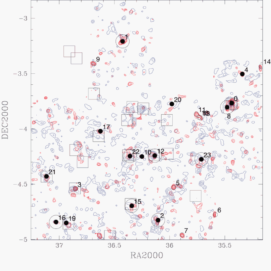
Figure 1: The $\kappa$-S/N map for the XMM-wide field (thick red contour). The lowest contour is set at S/N = 2 with the increments of 0.5. The smoothing scale, $\theta_{G}=1$ arcmin. The thin blue contours show the surface number density of visible (21$<R_{c}<$23) galaxies. Positions of detected halos (S/N $>=$ 3.693) are designated by small circles. Solid circles represent secure halos (see text) whereas unfilled circles represent samples detected outside the secure area. Squares show the location of X-ray selected clusters of galaxies published in Valtchanov et al. (2004), Willis et al. (2005) and Pierre et al. (2006). (VWP data). Large open circles show halos followed up by FOCAS and LRIS.

List of shear selected halos

Field	n	ID	RA	DEC	$\kappa$S/N	$\kappa$	Ng	FOCAS	Known	NEDG	Note
DEEP02	00	-	37.32	0.63	4.44	0.099	16	-	-	1.35
	01	-	37.87	0.51	4.39	0.083	24	-	-	-
	02	-	37.38	0.41	4.25	0.120	19	-	-	0.73
	04	-	37.15	0.73	4.11	0.086	25	-	-	0.10
	05	-	37.31	0.44	4.07	0.131	20	-	-	1.03
	06	-	37.72	0.69	3.97	0.081	18	-	-	0.86
	07	-	37.86	0.57	3.95	0.074	18	-	-	0.92
	08	SL J0228.4+0030	37.12	0.51	3.93	0.085	49	-	0.46(P)	-	VGCF 46
	09	SL J0228.2+0033	37.07	0.55	3.84	0.102	33	-	0.50(P)	-	SDSS CE J037.099808+00.540769
SXDS	00	-	34.29	-5.59	5.33	0.057	26	-	-	-
	01	-	34.38	-4.86	4.14	0.084	24	-	-	-
	02	-	34.61	-4.41	3.96	0.059	16	-	-	-
	03	-	34.74	-4.70	3.90	0.044	19	-	-	-
	04	-	34.96	-5.12	3.86	0.069	21	-	-	-
	05	-	34.41	-4.50	3.77	0.056	26	-	-	-
XMM-Wide	00	SL J0221.7-0345	35.44	-3.77	8.15	0.156	72	-	0.43	-	XLSSC 006
	01	SL J0225.7-0312	36.43	-3.21	5.72	0.108	41	0.14	-	-	LRIS z = 0.14
	02	SL J0224.4-0449	36.10	-4.82	5.06	0.074	40	0.49	-	-
	04	-	35.34	-3.50	4.91	0.082	21	-	-	-
	08	SL J0222.3-0446	35.48	-3.80	4.33	0.081	29	-	-	-	LRIS z = 0.41
	10	-	36.25	-4.25	4.20	0.062	23	-	-	-
	12	SL J0224.5-0414	36.13	-4.24	4.06	0.057	70	0.26	-	-	LRIS z = 0.26
	15	SL J0225.3-0441	36.34	-4.70	3.94	0.091	34	0.26	-	-
	16	SL J0228.1-0450	37.03	-4.84	3.94	0.072	31	0.29	-	-
	17	SL J0226.5-0401	36.63	-4.02	3.90	0.079	37	-	0.34	-	XLSSC 014
	19	SL J0227.7-0450	36.94	-4.85	3.81	0.064	43	-	0.29	-	Pierre et al. (2006)
	20	-	35.98	-3.77	3.81	0.048	20	-	-	-
	21	SL J0228.4-0425	37.12	-4.43	3.80	0.055	49	-	0.43	-	XLSSC 012
	22	SL J0225.4-0414	36.36	-4.25	3.72	0.073	43	0.14	-	-
	23	SL J0222.8-0416	35.71	-4.27	3.69	0.049	52	0.43,0.19,0.23	-	-
Lynx	00	-	131.91	44.80	5.84	0.121	20	-	-	-
	01	-	132.59	44.07	5.01	0.083	43	-	-	-
	03	-	131.83	44.86	4.57	0.139	23	-	-	-
	05	-	131.77	44.85	4.37	0.110	13	-	-	-
	07	-	132.69	44.95	4.15	0.105	31	-	-	-
	08	SL J0850.5+4512	132.64	45.20	4.02	0.085	53	0.19	0.24(P)	-	NSC J085029+451141,LRIS$z=0.19$
	09	-	131.47	44.96	4.02	0.076	26	-	-	-
	10	-	133.02	44.14	4.00	0.108	23	-	-	-
	12	-	132.37	44.38	3.90	0.081	36	-	-	-
	13	-	132.41	44.37	3.90	0.072	31	-	-	-	Part of n=12
	14	-	132.54	44.07	3.86	0.066	48	-	-	-
	15	-	132.81	44.35	3.77	0.077	39	-	-	-
	16	-	132.31	44.30	3.75	0.072	44	-	-	-
	17	-	131.40	44.94	3.74	0.084	25	-	-	0.15
COSMOS	00	SL J1000.7+0137	150.19	1.63	6.11	0.113	64	0.22	0.20(P)	-	NSC J100047+013912
	01	SL J1001.4+0159	150.35	1.99	5.64	0.098	32	-	0.85(P)	-	Finoguenov et al. (2006)
	02	SJ J0959.6+0231	149.92	2.52	4.74	0.067	83	-	0.73(P)	-	Finoguenov et al. (2006)
	05	-	149.65	1.55	3.92	0.078	47	-	-	-
	07	-	150.19	2.01	3.88	0.070	36	-	-	-

List of shear selected halos (continued from Table 2.6)

Field	n	ID	RA	DEC	$\kappa$S/N	$\kappa$	Ng	FOCAS	Known	NEDG	Note
Lockman	00	SL J1057.5+5759	164.39	58.00	6.28	0.109	68	0.60	-	-
	03	SL J1051.5+5646	162.88	56.77	4.97	0.082	31	0.33, 0.35	-	-
	05	SL J1047.3+5700	161.84	57.01	4.56	0.103	56	0.30, 0.24	-	-
	06	SL J1049.4+5655	162.35	56.93	4.51	0.095	47	0.42	-	-	LRIS z = 0.31
	09	SL J1055.4+5723	163.86	57.38	4.22	0.086	20	-	-	-	LRIS z = 0.38
	10	SL J1051.6+5647	162.92	56.78	4.20	0.068	49	0.33, 0.25	-	0.05	part of SL J1051.5+5646
	11	SL J1053.4+5720	163.35	57.34	4.08	0.064	50	-	0.34	-	RX J1053.3+5719
	12	-	163.69	57.55	4.07	0.068	26	-	-	-
	13	-	162.91	58.02	4.04	0.089	21	-	-	0.08
	14	-	162.54	57.28	3.93	0.070	38	-	-	-
	15	SL J1048.1+5730	162.04	57.51	3.89	0.071	35	0.32	-	-
	16	-	163.85	57.95	3.83	0.072	24	-	-	0.02
	18	-	163.16	57.88	3.77	0.069	26	-	-	-
	19	-	164.21	57.70	3.77	0.070	22	-	-	-
	20	-	163.23	57.84	3.73	0.102	29	-	-	-
	21	-	163.14	57.82	3.72	0.111	19	-	-	-
GD140	00	SL J1135.6+3009	173.91	30.16	4.98	0.126	35	0.21	-	-
	01	-	173.89	30.21	4.19	0.086	23	-	-	-
	02	-	173.96	29.81	4.09	0.069	17	-	-	-
	03	SL J1136.3+2915	174.09	29.26	4.03	0.100	24	-	-	-	LRIS z = 0.20
	05	-	174.77	29.89	3.86	0.111	26	-	-	-
	06	-	174.86	30.33	3.83	0.080	21	-	-	-
PG1159-035	05	SL J1201.7-0331	180.44	-3.53	4.42	0.077	49	0.52	-	-
	06	-	180.99	-3.09	3.90	0.119	21	-	-	0.09
	08	-	181.76	-3.27	3.71	0.102	37	-	-	-
13 hr Field	00	SL J1334.3+3728	203.60	37.47	4.33	0.128	74	0.30	0.48(P)	-	NSCS J133424+372822
	01	SL J1335.7+3731	203.94	37.53	4.10	0.091	65	0.41	-	-
	04	SL J1337.7+3800	204.43	38.01	3.85	0.080	34	0.18	-	-
	06	-	203.85	37.90	3.78	0.068	27	-	-	-
	07	-	204.22	37.54	3.77	0.078	30	-	-	-
GTO 2deg2	00	SL J1602.8+4335	240.72	43.59	6.65	0.110	56	0.42	-	-
	01	SL J1603.1+4245	240.78	42.76	5.47	0.106	57	-	-	-	LRIS z = 0.18
	02	-	241.82	43.19	5.17	0.133	21	-	-	-
	04	-	241.95	43.60	4.49	0.093	17	-	-	-
	07	SL J1604.1+4239	241.04	42.65	4.19	0.083	39	-	-	-	LRIS z = 0.30
	08	-	241.63	43.61	4.16	0.093	25	-	-	-
	09	SL J1605.4+4244	241.36	42.74	4.09	0.064	36	0.22	-	-
	10	-	241.18	43.46	3.85	0.092	29	-	-	-
	11	-	241.70	43.64	3.84	0.077	33	-	-	-
	12	SL J1603.1+4243	240.78	42.72	3.82	0.091	37	-	-	-	Part of SL J1603.1+4245
CM DRA	04	SL J1639.9+5708	249.98	57.15	4.15	0.073	32	0.20	-	-
	06	SL J1634.1+5639	248.55	56.66	3.97	0.104	31	0.24	-	-
DEEP16	00	SL J1647.7+3455	251.94	34.93	4.30	0.084	42	0.26	-	-
	01	-	253.54	34.98	4.24	0.078	24	-	-	-
	02	-	252.36	35.02	3.75	0.123	25	-	-	-
	03	-	251.79	35.04	3.72	0.087	21	-	-	-
DEEP23	00	SL J2326.4+0012	351.61	0.20	4.41	0.076	19	0.28	-	-
	01	-	351.75	0.00	4.37	0.095	20	-	-	-
	02	-	352.33	0.15	4.27	0.107	33	-	-	1.38
	03	-	352.47	-0.06	4.11	0.079	34	-	-	0.07
	04	-	352.22	0.09	3.87	0.084	21	-	-	1.37
	05	-	353.09	0.04	3.70	0.066	22	-	-	-

=8.5cmf8.eps

Faint galaxy density ($\rho_{gal}$) dependence of number density of secured halos (S/N $>$ 3.69) in each field. The error bars are based on $\sqrt{N}$ error estimates. Solid lines shows the predicted halo number density. The galaxy distribution is assumed ${dn\over{dz}}={\beta\over{z_{\ast}\Gamma[(1+\alpha)/\beta)]}}\left({z\over{z_{\ast}}}\right)^{\alpha}\exp\left[-\left({z\over{z_{\ast}}}\right)^{\beta}\right]$ where $\alpha=2.0$ and $\beta=1.5$ is adopted. The mean redshift, $\langle z\rangle$ is related to $z_{\ast}$ by $\langle z\rangle=z_{\ast}\Gamma[(2+\alpha)/\beta]/\Gamma[(1+\alpha)/\beta]$ Three different $\langle z\rangle$ are assumed; 0.8, 1.0 and 1.2 (from bottom to the top solid line).

Here we compare the detected halo number density [deg^-2] with the prediction of numerical simulations done by Hamana et al. (2004), who have attempted to reproduce a survey such as ours. Figure 2.6 shows the halo density of our thirteen survey fields. The horizontal axis shows the density of faint galaxies ($\rho_{gal}$) used for weak lensing analysis. The error bars are based only on $\sqrt{N}$ estimates and do not include the effects of cosmic variance. Solid lines in Figure 2.6 show the prediction of the simulation where three different mean redshifts for the background galaxies are assumed (from bottom to top: 0.8, 1.0 and 1.2).

Although the scatter is large, there is reasonable agreement between the observations and the prediction. We also see a gradual increase of the observed number density over the $\rho_{gal}$ range sampled as expected. These comparisons validate our observational procedures. We have, however, two outliers in Figure 2.6. These could be caused by cosmic variance or may arise from some other reasons. Further follow-up studies will be important to clarify the issue.

3 Cluster Identification and Verification

Armed with the shear-selected halo catalog, we now discuss the tests we have made to verify its reliability, using both spectroscopic observations and comparisons with X-ray data in the fields where the overlap of targets can be studied.

3.1 Spectroscopic Follow-up

Because the lensing kernel (or window function) has a relatively broad redshift range, the superposition of multiple low mass halos with different redshifts could yield highly significant weak lensing signals. Such ‘superposition halos’ are unwelcome in a mass-selected cluster catalog. In order to identify such superposition halos we undertook a more comprehensive spectroscopic survey using a multi-object spectrograph for selected candidates. This also gives us the velocity dispersion of member galaxies, which is an estimate of dynamical mass of clusters. By comparing dynamical mass with weak lensing mass we will be able to discuss the dynamical state of the clusters (Hamana et al. in preparation).

We used the FOCAS spectrograph on Subaru whose multi-object mode permits the simultaneous observation of 25 - 30 galaxies in the field of a particular halo. We used the 150/mm grating and a SY47 order sorting filter. This configuration spans the wavelength range $4700-9400$Å (Kashikawa et al., 2002). Target selection was based primarily on apparent magnitude and the color information was used when available. The exposure time was 45 $\sim$ 70 minutes depending on the magnitude of the selected galaxies and the observing conditions. The spectroscopic data was reduced using standard IRAF procedures (Hamana et al. in preparation). Figure 3.1 shows a typical FOCAS observation where the target is identified as a $z$ = 0.6 cluster.

(a) $\kappa$ S/N contour map of the most significant halo in the Lockman field (SL J1057.5+5759) superimposed on the $R_{c}$-band image taken by Suprime-Cam. Contours start at a S/N = 2 2 with an interval of 1. Small circles show the positions of observed galaxies by FOCAS with the redshifts obtained. (b) Redshift ‘cone diagram’ of the observed galaxies.

Since May 2004 we have observed 26 halos from the secure sample with FOCAS. Higher priority was given to more significant halos, except in the early stages of program (for example in the Lynx and PG1159-035 fields) when the follow-up strategy was still being evaluated. Each of the 26 halos has been reliably identified with a cluster of galaxies. The redshift so determined is shown in the column labeled “FOCAS” of Table 2.6,2.6.

In parallel with the FOCAS follow-up, long slit observations with Keck/LRIS have been carried out to enlarge the sample of redshifts as quickly as possible. We have to keep in mind that this method cannot discriminate the projected samples, and some statistical consideration is necessary in dealing with the data for further studies. A complete discussion of that aspect of our program is discussed in a separate paper (Green et al, in prep.). In the “Note” column of Table 2.6,2.6, we list the preliminary Keck/LRIS results as “LRIS z = zvalue” whose identification is already robust (e.g. at least two galaxy redshifts agree) including one of the halos in the XMM-Wide field (SL J0222.3-0446, $z$=0.41) where we discuss the reliability of our catalog (see section 3.3).

3.2 Correlation with Published Data

In addition to undertaking our own spectroscopic observations, we also searched the NASA Extragalactic Database (NED) for clusters and groups with published redshifts close to the position of our detected halos. We included recently-published cluster catalogs in the XMM-wide survey by Valtchanov et al. (2004), Willis et al. (2005) and Pierre et al. (2006) (VWP data hereafter). In making assignments, we considered a cluster to be associated with a halo if the angular separation was less than 2 arcmin and the 3 dimensional distance less than 1 $h^{-1}$ Mpc. 13 out of 100 halos can be identified in this way with rich clusters in the literature and the published redshift is shown in the column labeled “Known” of Table 2.6,2.6. Three of these thirteen clusters were also observed by FOCAS in multi-object mode and we note that the mean FOCAS redshift is different from the published value for these systems ($\delta z=0.02\sim 0.18$). These discrepancies can be explained by the fact that NED redshift of these clusters are all photometric, which have larger uncertainties. Therefore, we adopted the FOCAS redshifts for these three cases. We searched the NED galaxy group catalog in the same manner, but no group matched any of our halos.

Next, we searched for individual galaxies with published redshifts within 3 arcmin of our halos. If suitable data was found, we grouped them together using a “friend of friend” algorithm with a linking length of 1 $h^{-1}$ Mpc. If we found a clustering of more than two members, we calculated the average redshift and the mean astrometric position. Using the same proximity criterion above, we assigned a redshift to 14 further halos. These are shown in the column labeled “NEDG”.

In order to estimate the probability of a chance coincidence of the matching procedures, we first randomized the position of the detected halos in the field, and applied the same matching procedure described above to the randomized halo catalog. This process suggests that the probability of a chance coincidence is roughly 10 % and 25 % for the cluster and galaxy clustering searches, respectively. Clearly care should be taken in analyzing such data. The total number of reliably identified clusters are 41 (out of 100 in Table 2.6,2.6) where we do not include those identified by “NEDG” galaxies because the chance coincidence is not negligible. We assign ID labels only for these reliable halos in the tables.

3.3 Reliability of the Shear-Selected Halo Catalog

We now turn to the important question of the evaluating the reliability of our shear-selected catalog. We will do this by examining both the success rate of our identifications and by comparing with X-ray samples obtained via the XMM-Wide field survey. VWP have confirmed spectroscopic redshifts for 28 X-ray selected clusters in the 3.5 deg² survey field. Their locations are plotted as squares on Figure 1. Our secure sample of 15 shear-selected halos with S/N $>$ 3.69 is plotted as solid circles. Those we have spectroscopically confirmed using Subaru’s FOCAS and/or Keck LRIS are marked by large open circles. We find that three halos (1, 16 and 23) are confirmed as clusters by FOCAS and are not reported in VWP.

Among our 15 shear-selected halo samples, only three (4, 10 and 20) have yet to be identified. This identification success rate (80 %) can be regarded as a lower limit given future observations may yet locate an associated cluster. Although affected by small number statistics, this minimum efficiency is already higher than expected by simulation studies(White et al., 2002; Hamana et al., 2004; Hennawi & Spergel, 2005).

It is interesting to compare our identification success rate with those found in the GaBoDS survey. Maturi et al. (2006) found 14 significant halos in their 18 deg² area. Among them, 5 halos turn out to be known clusters of galaxies, 2 seem to have associated light concentrations but no spectroscopic confirmation, and the remaining uncertain 7 (50 %) had no apparent counterpart in either optical nor X-ray data. Schirmer et al. (2006) undertook a search on the same data adopting a different peak selection algorithm and a lower detection threshold. They found 158 “possible mass concentration” on the 18 deg² field. If those halos are divided into the same classes as above (known, light, uncertain), the ratio is almost the same as Maturi et al. (2006). Regardless, almost half of the GaBoDS halos could be considered uncertain at this point.

Meanwhile, we find 15 halos in a 2.24 deg² field (XMM-wide) and show that 80 % of have been already identified as clusters. It is too early to make any definite conclusion because their spectroscopic is underway. However, our (tentatively) higher success rate could be explained at least in part by the larger number density of faint galaxies, $\rho_{gal}$, usable for the weak lensing analysis owing to larger aperture and better average seeing. In the case of GaBoDS, $\rho_{gal}$ spans from 6 to 28 arcmin^-2 depending on the field; the average value is 11 arcmin^-2. This is generally smaller than our $\rho_{gal}$ shown in Table 1. As a result one can expect a lower angular resolution of the $\kappa$ map, reducing the S/N ratio for a fixed smoothing scale and possibly an increased degree of contamination in the resulting halo catalog. Another possibility to explain the increased contamination is that their sample consists of a combination of different sets of catalogs, each of which is selected by different methods. This could decrease the significance threshold effectively, and could introduce more false peaks.

3.4 Superposition of Multiple Clusters

Hamana et al. (2004) estimated, based on their simulation, that the halo superposition rate in survey such as ours should be roughly 3 % - a small but not negligible effect. A longslit spectroscopic survey, such as that undertaken with LRIS (Green et al, in prep) might be poorly-suited for locating such cases. However, the FOCAS multi-object survey reported here should reliably find them. In fact, we have found three apparent superposition halos (SL J0222.8-0416, SL J1051.5+5456 and SL J1047.3+5700) out of 26 examined. The overlap rate is broadly consistent with expectation considering the small number so far sampled.

4 Conclusions and Future Prospects

We have introduced a new Subaru imaging survey and described techniques for locating and verifying shear-selected halos. Across a search area of 16.72 deg² we have found 100 halos whose $\kappa$ S/N exceeds 3.69. We have described the first phase of a detailed follow-up campaign based on multi-object spectroscopy of 26 halos using FOCAS on the Subaru telescope. A later paper in this series (Green et al, in prep) will extend the spectroscopic survey to the full sample using a longslit approach.

Detailed studies on one of our fields, the XMM-wide field, show that 80% of the shear selected 15 halos in the 2.2 deg² area can be confirmed as genuine clusters of galaxies. 10 overlap with X-ray detections and two are new systems confirmed spectroscopically. The overall success rate and reliability of our sample provides convincing proof that, with care, a weak lensing survey can provide a large sample of mass-selected halos.

We compare our success rate and the reliability of our catalog with that of the GaBoDS survey and conclude a major advantage of our approach is the superior imaging depth which leads to a high surface density of usable galaxies. This suggests future, more ambitious, surveys for shear-selected halos will be more effective if undertaken with large aperture telescopes.

It is interesting to use our results to estimate the requirements for a future survey motivated by the need to constrain dark energy. Kolb et al. (2006) discuss hypothetical missions which would aim to analyze the redshift distribution $N(z)$ of 10,000 clusters. Figure 2.6 shows that our survey technique typically finds 5 halos deg^-2. Because the field size of Suprime-Cam is $\sim$ 0.25 deg², it takes two hours to cover 1 deg² assuming the exposure time of 30 minutes of each field as adopted in this study. A survey of 10,000 clusters would be prohibitive even in terms of imaging alone ($\sim$ 500 clear nights) even before contemplating the follow-up spectroscopy. The Hyper Suprime-Cam (HSC) project (Miyazaki et al., 2006) has been proposed to remedy this shortcoming. HSC is expected to have a field of view ten times larger than Suprime-Cam while maintaining the same image quality. This new facility will makes the 2000 deg² scale imaging survey within a reasonable number of clear nights.

Spectroscopic follow-up might be enabled by the proposed prime focus multi object optical spectrograph WFMOS (Wide Field Fiber Multi Object Spectrograph) whose field is 1.5 deg² in diameter. Typically we can expect $\simeq$10 shear-selected clusters in each spectroscopic field. With only 20 targets per halo, only a small fraction of the several thousand fibers envisaged for WFMOS need be allocated to the halo verification program.

=4.151cmf10.eps

DEEP02 field $\kappa$-S/N map (red contour) and surface number density of moderately bright (21$<R_{c}<$23) galaxies (blue contour). Legends are the same as Fig 1.

=9.296cmf11.eps

SXDS field $\kappa$-S/N map and surface density of galaxies. (blue contour).

=11.00cmf12.eps

Lynx field $\kappa$-S/N map and surface density of galaxies.

=10.507cmf13.eps

COSMOS field $\kappa$-S/N map and surface density of galaxies.

=10.264cmf14.eps

Lockman field $\kappa$-S/N map and surface density of galaxies.

=9.458cmf15.eps

GD140 field $\kappa$-S/N map and surface density of galaxies.

=9.466cmf16.eps

PG1159-035 field $\kappa$-S/N map and surface density of galaxies.

=9.462cmf17.eps

13 hr field $\kappa$-S/N map and surface density of galaxies.

=9.465cmf18.eps

GTO 2 square degree field $\kappa$-S/N map and surface density of galaxies.

=9.466cmf19.eps

CM DRA field $\kappa$-S/N map and surface density of galaxies.

=4.326cmf20.eps

DEEP16 field $\kappa$-S/N map and surface density of galaxies.

=4.145cmf21.eps

DEEP23 field $\kappa$-S/N map and surface density of galaxies.

Appendix A Probability to obtain spurious peaks due to insufficient correction of the PSF anisotropy

The shear induced by massive cluster of galaxies is expected to be 7$\sim$ 10 %. This is actually larger than raw ellipticities due to PSF anisotropy (2 $\sim$ 4 % refer to Fig. 2.2), but the difference is not so significant. Therefore, the correction of the anisotropy is very important to make a precise kappa map. Here, we examine the PSF anisotropy Suprime-Cam, and evaluate the effect of imperfect correction in this work.

=17cmf22.eps

Two examples of ellipticities field. Orientation of each bar shows the direction of the major axis, and the length scales as its ellipticity. No subtraction of the offset is made. Arrow on left top of the panel shows the size of 10 % ellipticity. The seeing was 0.65 arcsec (FWHM).

In order to characterize the anisotropy of the Suprime-Cam images, we obtained sequences of i’-band short exposures (1 min) of dense stellar fields with various telescope pointings over one night long. The seeing was mostly $\sim$ 0.65 arcsec (FWHM). The PSF anisotropy is approximated as an elliptical, and the field position dependence of the ellpticities are investigated. Two examples of such ellipticity fields are shown in Fig. A. General tendency that we note is that the fields can be represented as a super-position of (1) the radial field at four corners (almost invariant) and (2) almost unidirectional field (variable). The variable components is most likely due to the telescope shaking whereas the invariant component can be explained by the optical aberration of the corrector. Slight asymmetry of the radial component is visible (i.e. ellipticities near the lower left corner is larger than other corners), and this would be a sign of imperfect optical alignment.

=17cmf23.eps

(a) Ellipticities of stars azimuthally averaged over the field of view (0.65 arcsec seeing i’-band 60 sec exposure). Open circle and square show the results of “before” and “after” the anisotropy correction, respectively (see text). Sold squares show expected ellipticities from perfectly aligned optics under the seeing of 0.65 arcsec. (b)Peak distribution function of kappa S/N map created by residual of anisotropy corrections.

We also note that the discontinuity of ellipticities is not visible across the boundary of the CCDs, and the ellipticities can be represented as a single continuous function of field position. We adopt 5-th order polynomial function here. In order to simulate the actual science field analysis, we randomly select controls stars and “galaxy role” stars from the star catalogs with an appropriate density; 2 arcmin^-1 and 40 arcmin^-1, respectively. Using the control stars, we obtain the best fit coefficients of the polynomial, and the anisotropy of “galaxy role” stars is corrected using Eqn. 2. Because the intrinsic ellipticities of “galaxy role” stars is all zero, the residual ellipticities after the correction is a estimate of incompleteness of the correction. Fig A(a) shows the azimuthally averaged ellipticities of stars; before the correction, the typical 3 % raw ellipticity is seen. It might be interesting to note that the ellipticities of 3 %. can be induced by rms pointing error of merely 0.1 arcsec under the seeing of 0.65 arcsec. The ellipticities is reduced down to about 0.75 % after the correction. Beyond the field angle of 18 arcmin, the correction does not work fine and we decided to eliminate the field r $>$ 18 from lensing analysis; which, however, results in only a few percent loss of FOV.

We estimated a PSF anisotropy caused by the optical aberration using a ray-tracing code, zemax. The calculated PSF is convolved with 0.65 arcsec FWHM gaussian, and the shape is evaluated by elliptical. The result is shown in filled square in Fig A(a). Compared with this ideal case, the observed ellipticities is large even after the correction. This shows a limit of the adoption of single polynomial function as a representatives of the PSF anisotropy, where the residual is still locally correlated correlated and not completely random. We now want to evaluate the impact of the incompleteness onto the $\kappa$ S/N map. The map is created based by the residual ellipticities after the correction. We simulate the galaxy ellipticities using the following “conversion” formula (Hoekstra, 2004),

$$e^{gal}=\frac{P_{sm}^{gal}}{P_{sm}^{*}}e^{*},$$ (A1)

which is essentially a sensitivity correction against the PSF anisotropy. This is necessary because galaxies are larger and their shape is more insensitive to the deformation compared with stars. We evaluate $\frac{P_{sm}^{gal}}{P_{sm}^{*}}$ with $\frac{\langle Tr(P_{sm}^{gal})\rangle}{\langle Tr(P_{sm}^{*})\rangle}$ where we adopt $\langle Tr(P_{sm}^{gal})\rangle=0.1$ which is a typical value under the typical 0.7 arcsec seeing. Since the $\langle Tr(P_{sm}^{*})\rangle\sim 0.2$ here, the conversion factor is roughly $\frac{1}{2}$. We omit $P_{\gamma}$ correction because it cancels out in this case when we calculate the S/N. We created twelve such maps from independent exposures, and co-added the peak distribution functions to obtain Fig A(b). It is obvious that the incompleteness of the anisotropy correction is quite unlikely to create any significant (say S/N $>$ 3) fake peaks.

References

- Allen et al. (2003) Allen, S.W., Schmidt, R.W., Fabian, A.C., Ebeling, H. 2003 MNRAS342, 287
- Allen et al. (2004) Allen, S.W., Schmidt, R.W., Ebeling, H., Fabian, A.C., van Speybroeck, L. 2004 MNRAS, 353, 457
- Becker et al. (2007) Becker, M.R. et al. 2007 submitted to ApJ (astro-ph/0704.3614)
- Bernstein & Jarvis (2002) Bernstein, G. & Jarvis, M. 2002, AJ, 123, 583
- Böhringer et al. (2001) Böhringer, H. et al. 2001 A&A, 369, 826
- Davis et al. (2003) Davis, M., Faber, S.M., Newman, J. et al. 2003, SPIE, 4834, 161
- Dietrich et al. (2007) Dietrich, J.P., Erben, T., Lamer, G., Schneider, P., Schwope, A., Hartlap, J., Maturi, M (2007) A&A in press (astro-ph/0705.3455)
- Erben et al. (2001) Erben, T., van Waerbeke, L., Bertin, E., Mellier, & Y. & Schneider, P. 2001, A&A, 366, 717
- Finoguenov et al. (2006) Finoguenov, A., Guzzo, L., Hasinger, G., Scoville, N.Z. et al. (2006) ApJS in press (astro-ph/0612360)
- Gladders & Yee (2000) Gladders, M.D. & Yee, H.K.C. 2000, AJ, 120, 2148
- Goto et al. (2002) Goto, T. et al. 2002, AJ, 123, 1807
- Hamana et al. (2003) Hamana, T., Miyazaki, S. et al. 2003, ApJ, 597, 98
- Hamana et al. (2004) Hamana, T., Takada, M., Yoshida, N. 2004, MNRAS, 350, 893
- Hennawi & Spergel (2005) Hennawi, J.F. & Spergel, D.N. 2005 ApJ, 624, 59
- Henry (2000) Henry, J.P. 2000, ApJ, 534, 565
- Hetterscheidt et al. (2005) Hetterscheidt, M., Erben, T., Schneider, P., Maoli, R., van Waerbeke, L., Mellier, Y. 2005, A&A, 442, 43.
- Heymans et al. (2006) Heymans, C. et al. 2006, MNRAS, 368, 1323
- Hoekstra et al. (1998) Hokekstra, H., Franx, M., Kuijken, K., Squires, G. 1998 ApJ, 504. 636
- Hoekstra (2004) Hoekstra, H. 2004, MNRAS, 347, 1337
- Ikebe et al. (2002) Ikebe, Y., Reiprich, T.H., Böhringer, H., Tanaka, Y., Kitayama, T. 2002 A&A, 383, 773
- Jenkins et al. (2001) Jenkins, A., Frenk, C. S., White, S. D. M., Colberg, J. M., Cole, S., Evrard, A. E., Couchman, H. M. P. & Yoshida, N. 2001, MNRAS, 324, 450
- Kaiser & Squires (1993) Kaiser, N. & Squires, G. 1993, ApJ, 404, 441
- Kaiser et al. (1995) Kaiser, N., Squires, G. & Broadhurst, T. 1995, ApJ, 449, 460
- Kaiser et al. (1999) Kaiser, N., Wilson, G., Luppino, G., Dahle, H. 1999 submitted to PASP (astro-ph/9907229)
- Kashikawa et al. (2002) Kashikawa, N. et al. 2002, PASJ, 54, 819
- Kolb et al. (2006) Kolb et al. 2006, US Dark Energy Task Force Report
- Landolt (1992) Landolt, A.U. 1992, AJ, 104, 340
- Levine et al. (2002) Levine, E.S., Schulz, A.E., White, M. 2002 ApJ, 577, 569
- Luppino & Kaiser (1997) Luppino, G.A. & Kaiser, N. 1997, ApJ, 475, 20L
- Majewski et al. (1994) Majewski, S.R., Kron, R.G., Koo, D.C., Bershady, M.A. 1994, PASP, 106, 1258
- Massey et al. (2007) Massey, R.J, Rhodes, J., Ellis, R.S. et al 2007, Nature, 445, 286
- Maturi et al. (2006) Maturi, M., Schirmer, M., Meneghetti, M., Bartelmann, M., Moscardini, L. 2006, A&A in press (astro-ph/0607254)
- Miyazaki et al. (2002a) Miyazaki, S., Hamana, T., Shimasaku, Furusawa, H., Doi, M., Hamabe, M., Imi, K., Kimura, M., Komiyama, Y., Nakata, F., Okada, N., Okamura, S., Ouchi, M., Sekiguchi, M., Yagi, M., Yasuda, N. 2002a ApJ, 580, L97
- Miyazaki et al. (2002b) Miyazaki, S., Komiyama, Y., Okada, N., Imi, K., Yagi, M., Yasuda, N., Sekiguchi, M., Kimura, M, Doi, M., Hamabe, M., Nakata, F., Shimasaku, K., Furusawa, H., Ouchi, M. & Okamura, S. 2002b, PASJ, 54, 833
- Miyazaki et al. (2006) Miyazaki, S., Komiyama, Y., Nakaya, H., Doi, Y., Furusawa, H., Gillingham, P., Kamata Y., Takeshi, K., Nariai, K. 2006, SPIE, 6269, 9
- Pierre et al. (2004) Pierre, M. et al. 2004 J. Cosmol. Astropart. Phys, 09, 011
- Pierre et al. (2006) Pierre, M., Pacaud, F. et al. 2006, MNRAS, 372, 591
- Postman et al. (1996) Postman, M., Lubin, L.M., Gunn, J.E., Oke, J.B., Hoessel, J.G., Schneider, D.P., Christensen, J.A. 1996, AJ, 111, 615
- Press et al. (1993) Press, W.H., Flannery, B.P., Teukolsky, S.A., Vetterling, W.T. 1993, “Numerical Recipes in C”, ISBN-13: 9780521431088
- Reiprich & Böhringer (2002) Reprich, T.H. & Böhringer, H. 2002 ApJ, 567, 716
- Schirmer et al. (2006) Schirmer, M., Erben, T., Hetterscheidt, M., Schneider, P. 2006, Submitted to A&A (astro-ph/0607022)
- Smail et al. (1997) Smail, I., Ellis, R.S., Dressler, A. et al. 1997 ApJ, 479, 70
- Smith et al. (2005) Smith, G.P., Kneib, J., Smail, I., Mazzotta, P., Ebeling, H., Czoske, O. 2005, MNRAS, 359, 417
- Valtchanov et al. (2004) Valtchanov, I. et al. 2004, A&A, 423, 75
- Wang et al. (2004) Wang, S., Khoury, J., Haiman, Z. May, M. 2004 PhRvD, 70, 123008
- Van Waerbeke et al. (2000) Van Waerbeke, L., Mellier, Y., Erben, T. et al. 2000, A&A, 358, 30
- White et al. (2002) White, M., van Waerbeke, L, Mackey, J. 2002, ApJ, 575, 640
- Willis et al. (2005) Willis, J.P., Pacaud, F., Valtchanov, I. et al 2005, MNRAS, 363, 675
- Wittman et al. (2001) Wittman, D., Tyson, J.A., Margoniner, V.E., Cohen, J.G., Dell’Antonio, I.P. 2001 ApJ, 557, L89.
- Wittman et al. (2002) Wittman, D, Tyson, J.A., Dell’Antonio, I.P. et al. 2002, Proc, SPIE, 4836, 73
- Wittman et al. (2006) Wittman, D, Dell’Antonio, I.P, Hughes, J.P. et al. 2006, ApJ, 643, 128