The Cosmic Far-Infrared Background Buildup Since Redshift 2 at 70 and 160 microns in the COSMOS and GOODS fields.

Abstract

Context. The Cosmic Far-Infrared Background (CIB) at wavelengths around $160\leavevmode\nobreak\ \mu$m corresponds to the peak intensity of the whole Extragalactic Background Light, which is being measured with increasing accuracy. However, the build up of the CIB emission as a function of redshift, is still not well known.

Aims. Our goal is to measure the CIB history at 70 $\mu$m and 160 $\mu$m at different redshifts, and provide constraints for infrared galaxy evolution models.

Methods. We use complete deep Spitzer 24 $\mu$m catalogs down to about 80 $\mu$Jy, with spectroscopic and photometric redshifts identifications, from the GOODS and COSMOS deep infrared surveys covering 2 square degrees total. After cleaning the Spitzer/MIPS 70 $\mu$m and 160 $\mu$m maps from detected sources, we stacked the far-IR images at the positions of the 24 $\mu$m sources in different redshift bins. We measured the contribution of each stacked source to the total 70 and 160 $\mu$m light, and compare with model predictions and recent far-IR measurements made with Herschel/PACS on smaller fields.

Results. We have detected components of the 70 and 160 $\mu$m backgrounds in different redshift bins up to $z\sim 2$. The contribution to the CIB is maximum at $0.3\leq z\leq 0.9$ at 160$\mu$m (and $z\leq 0.5$ at 70 $\mu$m). A total of 81% (74%) of the 70 (160) $\mu$m background was emitted at $z<1$. We estimate that the AGN relative contribution to the far-IR CIB is less than about 10% at $z<1.5$. We provide a comprehensive view of the CIB buildup at 24, 70, 100, 160 $\mu$m.

Conclusions. IR galaxy models predicting a major contribution to the CIB at $z<1$ are in agreement with our measurements. The consistency of our results with those obtained through the direct study of Herschel far-IR data at 160 $\mu$m confirms that the stacking analysis method is a valid approach to estimate the components of the far-IR background using prior information on resolved mid-IR sources. Our results are available online http://www.ias.u-psud.fr/irgalaxies/ . [(…) abstract abridged]

1 Introduction

The Extragalactic Background Light (EBL) is the relic emission of galaxy formation and evolution, i.e. due to star formation and accretion processes (with this definition, the Cosmic Microwave Background due to recombination at redshift $z\sim$ 1100 is not part of the EBL). The EBL spectrum peaks in the Far-Infrared (FIR), where it is commonly known as the Cosmic Infrared Background (CIB) Puget et al. (1996); Hauser et al. (1998); Hauser & Dwek (2001); Kashlinsky (2005); Dole et al. (2006). The EBL and the CIB encode the emission processes of structure formation, and can thus be used to constrain the photon budget of the cooling processes leading the baryons to fall within the dark matter halos and form galaxies. The measurements of the EBL level and structure bring thus one of the many useful constraints for the models.

The CIB Spectral Energy Distribution is known with increasing accuracy (Puget et al., 1996; Aharonian et al., 2006; Dole et al., 2006; Bethermin et al., 2010, for instance in the FIR and submillimetre regime: ), but little is known about its history, i.e. its buildup as a function of redshift. This missing information should help constrain galaxy evolution models, and also better understand the physics of blazars, whose high-energy photons interact with the CIB along the line of sight (Aharonian et al., 2007; Albert & Magic Collaboration, 2008; Raue et al., 2009; Kneiske & Dole, 2009, e.g. ).

The history of the CIB buildup can be derived by integrating the luminosity functions of galaxies as a function of redshift (neglecting other sources of diffuse emission and thus assuming that the CIB is due to galaxies). This is a very difficult task in practice, since high-redshift luminosity functions are not yet measured at wavelengths close to the peak of the CIB (near 160 $\mu$m) but instead in the mid-infrared range (Le Floc’h et al., 2005; Caputi et al., 2007, e.g. ), or only in the local universe Soifer & Neugebauer (1991); Takeuchi et al. (2006). This situation is about to change with the latest Spitzer surveys and the ongoing deeper Herschel surveys Magnelli et al. (2009); Clements et al. (2010); Dye et al. (2010).

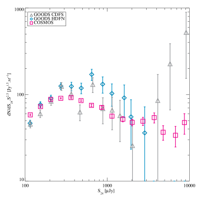
Figure 1: Number counts at 24 $\mu$m in the GOODS HDFN (blue diamond), GOODS CDFS (gray triangle) and COSMOS (pink square) fields. The errors bars used only include Poisson statistics, and not cosmic variance.

Two recent breakthroughs have been made by using COSMOS and GOODS surveys. Firstly, using about 30000 Spitzer 24 $\mu$m selected sources with accurate photometric redshifts Ilbert et al. (2009), Le Floc’h et al. (2009) were able to measure the 24 $\mu$m background buildup with redshift (e.g. their figures 7 to 9). They furthermore show that the redshift information is crucial when confronting data to the models, since it helps breaking degeneracies. Secondly, using the redshift identification of Herschel/PACS 100 and 160 $\mu$m sources, Berta et al. (2010) were able to measure the CIB build up in four redshift bins, in the 140 arcmin² GOODS-N field (an area about 40 times smaller than used in this analysis).

In this paper, we measure the 70 $\mu$m and 160 $\mu$m CIB history since $z=2$, with the use of a stacking analysis of galaxies detected at 24 $\mu$m (a good proxy for the 160 $\mu$m CIB population, e.g. Dole et al. (2006); Bethermin et al. (2010)) in the Spitzer data of the GOODS and COSMOS fields. This approach complements on a large area what is being done with Herschel in Berta et al. (2010) at 100 and 160 $\mu$m.

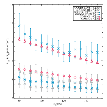
Figure 2: Cumulative stacked brightness at 70 $\mu$m and 160 $\mu$m (in nW.m^-2.sr^-1) on the CLEANed maps, as a function of the 24 $\mu$m flux of our sample, regardless of the redshift. the 3 fields are represented at 160 and 70 $\mu$m: COSMOS; GOODS-N (HDFN) and GOODS-S (CDFS).

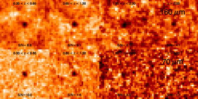
Figure 3: Images of all the stacked galaxies on the 160 $\mu$m (top) and 70 $\mu$m (bottom) GOODS CLEANed maps by redshift bin (right to left): 0$<$z$<$0.65; 0.65$<$z$<$1.3; 1.3$<$z$<$2 and z$>$2. The S/N ratio is indicated in each image. Notice the detection in the two first redshift bins at both wavelengths. Images are $305\times 305$ sq. arcsec. wide at 70 $\mu$m (with 9.85 arcsec pixel plate), and $496\times 496$ sq. arcsec. at 160 $\mu$m (with 16 arcsec pixel plate). The PSF FWHM being 18 arcsec. (resp. 40) at 70 $\mu$m (resp. 160 $\mu$m), the PSF shown on these figures has about the same extend of 1.8 to 2.5 pixels at both wavelengths.

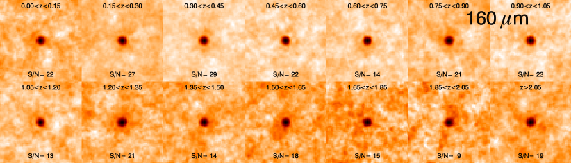
Figure 4: Images of all the stacked galaxies on the 160 $\mu$m COSMOS CLEANed maps with 14 redshift bins (left to right and top to bottom). The S/N ratio is indicated in each image. Notice the detection in all redshift bins at both wavelengths. Images are $488\times 488$ sq. arcsec. at 160 $\mu$m (with 8 arcsec pixel plate). The PSF FWHM of 40 arcsec. corresponds to 5 pixels on these images.

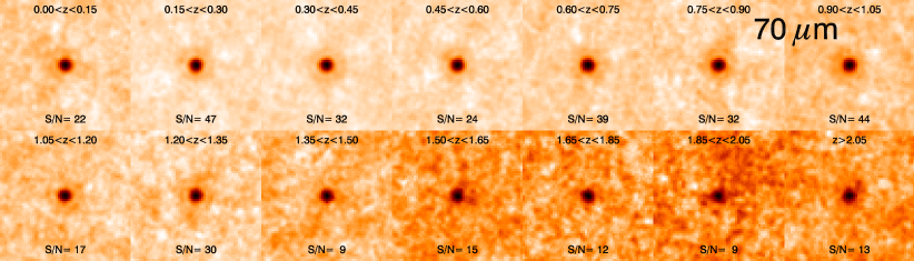
Figure 5: Images of all the stacked galaxies on the 70 $\mu$m COSMOS CLEANed maps with 14 redshift bins. Images are $244\times 244$ sq. arcsec. wide at 70 $\mu$m (with 4 arcsec pixel plate). The PSF FWHM of 18 arcsec. corresponds to 4.5 pixel on these images.

2 Data and Sample

2.1 GOODS data

The data were acquired by the MIPS imaging photometer at 24 $\mu$m, 70 $\mu$m and 160 $\mu$m Rieke et al. (2004) onboard the Spitzer infrared space telescope Werner et al. (2004), and come from the GOODS team Chary et al. (2004) and Guaranteed Time observations Papovich et al. (2004); Dole et al. (2004) of the Chandra Deep Field South (CDFS) and the Hubble Deep Field North (HDFN). Papovich et al. (2004) extracted a catalog at 24 $\mu$m, with 80% completeness at 80 $\mu$Jy. We use a sample of 1349 galaxies with 24 $\mu$m flux densities $S_{24}\geq 80\leavevmode\nobreak\ \mu$Jy, located in the two GOODS fields, north and south, for a total area of 291 Sq. Arcmin Caputi et al. (2006, 2007). The galaxies have been completely identified, and redshifts determined for all of them, with more than 45% of spectroscopic redshifts. Active Galactic Nuclei (AGN) are separated from the star-forming systems using X-ray data and near-infrared (3.6 to 8 $\mu$m) colors: we have 136 AGNs for 1213 star-forming systems Caputi et al. (2007). For our purpose of measuring the contribution of mid-infrared galaxies to the far-infrared background by redshift slice, we cut the 24 $\mu$m sample in four redshift bins: 0$<$z$<$0.65 with 317 sources (of which 9 AGNs), 0.65$<$z$<$1.3 with 575 sources (45 AGNs), 1.3$<$z$<$2 with 259 sources (38 AGNs) and z$>$2 with 198 sources (44 AGNs). These bins have been chosen to maximize the number of sources present in each bin, while keeping the same $\Delta z$ width.

Table 1: Number of 24 $\mu$m sources per redshift bins for the COSMOS field. $N_{tot}$ is the total number of galaxies used in the stacks, and $N_{AGNs}$ is the number of sources identified as AGN that were used in the stacks to estimate the AGN contribution.

z bin	0$<$ $z$ $<$0.15	0.15$<$z$<$0.3	0.3$<$ $z$ $<$0.45	0.45$<$z$<$0.6	0.6$<$ $z$ $<$0.75	0.75$<$z$<$0.9	0.9$<$ $z$ $<$1.05
$N_{tot}$	2083	1559	2853	2201	3225	3590	3478
$N_{AGNs}$	34	32	74	48	88	110	123
z bin	1.05$<$z$<$1.2	1.2$<$ $z$ $<$ 1.35	1.35$<$z$<$1.5	1.5$<$z$<$1.65	1.65$<$z$<$1.85	1.85$<$z$<$2.05	$z$ $>$2.05
$N_{tot}$	2670	1401	2044	1311	1519	2073	2833
$N_{AGNs}$	83	76	55	225	232	200	288

2.2 COSMOS data

The Cosmic Evolution survey (COSMOS) data were acquired by MIPS at 24, 70 and 160 $\mu$m. The 24 $\mu$m observations of the COSMOS field is part of two General Observer programs (PI D. Sanders): G02 (PID 20070) carried out in January 2006, G03 (PID 30143) carried out in 2007. We use a total net area of 1.93 Sq. degrees. Le Floc’h et al. (2009) extracted a catalogue at 24 $\mu$m and provided us a sample of 32840 galaxies with 24 $\mu$m flux densities $S_{24}\geq 80\leavevmode\nobreak\ \mu$Jy. The completeness limit is at the order of 90% at this level. (Notice that the survey sensitivities are similar in the COSMOS and GOODS fields, at 24, 70 and 160 $\mu$m). The 24 $\mu$m galaxies have been completely identified, and redshifts derived by Ilbert et al. (2009) and Salvato et al. (2009) for the optically and X-Ray selected sources of the COSMOS field. We use the Salvato et al. (2009) photometric redshift catalogue of the Cappelluti et al. (2009) X-Ray sources catalogue, optically matched by Brusa et al. (2007) Brusa et al. (2010) to identify the AGN in the COSMOS field (Le Floc’h et al., 2009). Notice that the X-ray flux limits used in the soft (0.5-2keV), hard (2-10keV) or ultra-hard (5-10keV) bands are $5\times 10^{-16}$, $3\times 10^{-15}$ and $5\times 10^{-15}$ erg cm^-2 s^-1, respectively Cappelluti et al. (2007, 2009); Salvato et al. (2009). We complete this sample with sources with a power-law SED Alonso-Herrero et al. (2006) in the redshift range 1.5$<$z$<$2.5 using IRAC colors (at lower and higher redshifts, the colors can be contaminated by the PAH or stellar bumps) in the same way as for the GOODS sample. We obtained 1668 sources (1115 X-Ray sources, 553 power-law sources) detected at 24 $\mu$m and identified as AGNs for 31172 star forming systems.

The COSMOS sample being larger than the GOODS one we used 14 redshift bins, described in table 1. The source statistics in these fields is summarized in Fig. 1, showing the number counts of the GOODS survey (CDFS and HDFN) as well as the COSMOS field, corrected for incompleteness. The errors bars used only include Poisson statistics, and not cosmic variance, and are thus likely underestimated. There is no evidence of a relative major over- or under-density, except maybe a slight over-density in the HDFN around 1 mJy, which has a negligible contribution to the total background.

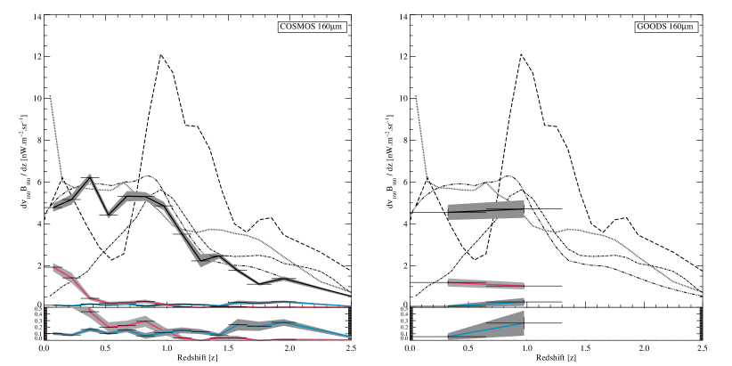
Figure 6: Differential 160 $\mu$m background brightness $d\nu_{160}B_{160}/dz$ as a function of redshift, in units of nW.m^-2.sr^-1, in the COSMOS field (left) and GOODS field (right). The lower part of the plot shows a linear zoom between 0 and 0.5 nW.m^-2.sr^-1 in order to exhibit the trend of cleaned sources and AGNs. Black solid lines: total contribution of infrared galaxies. Solid red lines: contribution from resolved sources only. Solid blue line: contribution from AGN only. Dash line Lagache et al. (2004) model, with $S_{24}>80\leavevmode\nobreak\ \mu$Jy cut. Dot line: Le Borgne et al. (2009) model, with $S_{24}>80\leavevmode\nobreak\ \mu$Jy cut. Dot-dash line:Valiante et al. (2009). Dot-dot-dot-dash line: Bethermin et al. (2010c) model, with $S_{24}>80\leavevmode\nobreak\ \mu$Jy cut. Models are discussed in Sect. 4.5 and figure 10.

3 Analysis

3.1 Stacking analysis

In order to estimate the contribution of mid-infrared galaxies to the 70 $\mu$m and 160 $\mu$m background, we make use of a stacking analysis Dole et al. (2006); Bethermin et al. (2010b). This method consists in stacking the 70 and 160 $\mu$m maps at the location of the galaxies detected at 24 $\mu$m. The use of this method is justified by two reasons. 1) The 24 $\mu$m population is a good proxy for the 70 $\mu$m and 160 $\mu$m populations making up most of the CIB near its peak Dole et al. (2006); Bethermin et al. (2010). 2) Only a few sources are individually detected at FIR wavelengths and do not resolve much of the background Dole et al. (2004); Frayer et al. (2006a, b); Dole et al. (2006); Frayer et al. (2009). Notice that stacking may suffer from the contamination of galaxy clustering, since the stacked image shows in two dimensions the 2 point angular correlation function Dole et al. (2006); Bavouzet (2008); Bethermin et al. (2010). However with the Spitzer and Herschel beams, the effects of clustering in the stacking are not important (less than 15%) Bavouzet (2008); Fernandez-Conde et al. (2008, 2010).

We first stack the 70 $\mu$m and the 160 $\mu$m MIPS data (CLEANed maps) as a function of the 24 $\mu$m flux, regardless the redshift of the sources (Fig. 2). This allows us to check the consistency of the procedure, since the total brightness measured for stacks down to $S_{24}=80\leavevmode\nobreak\ \mu$Jy should be equal to the sum of the brightnesses obtained by redshift slices, as well as identify possible biases. The stacks in the COSMOS and the two GOODS fields at 70 and 160 $\mu$m show strong dependencies on the fields: while COSMOS and GOODS-N (HDFN) stacks are consistent within 20%, stacks in CDFS field is systematically lower than COSMOS by a factor of about 1.4-1.8. The better statistics in the COSMOS field (surface area and number of sources) is limiting the impact of the variance due to the large scale structure, and we attribute the systematic lower values in GOODS-S to this effect.

Prior to stacking the 24 $\mu$m catalog in redshift bins on the 70 $\mu$m and 160 $\mu$m maps, we use the clean algorithm Hogbom (1974) to subtract the few resolved sources present in the Far-Infrared maps, in order to remove any bias in the resulting photometry of the stacked images. The stacking analysis presented on Fig. 2 was also done on the cleaned Far-Infrared maps. In the COSMOS field, we clean the sources brighter than 80 mJy (resp. 20 mJy) at 160 $\mu$m (resp. 70 $\mu$m), level corresponding to 90 to 95% completeness, levels computed by Monte-Carlo simulations on the data themselves Bethermin et al. (2010). In both GOODS fields, we removed all the detected sources at 160 $\mu$m $\&$ 70 $\mu$m identified at 24 $\mu$m. It corresponds to sources brighter than 19 mJy at 160 $\mu$m (5 sources in GOODS HDFN $\&$ 12 sources in GOODS CDFS) and 4.4 mJy at 70 $\mu$m (8 sources in GOODS HDFN $\&$ 17 sources in GOODS CDFS). These brightest detected sources at 70 and 160 $\mu$m have been individually identified at 24 $\mu$m without ambiguity, and the redshift of the 24 $\mu$m source is used. The flux densities of the removed detected sources are converted into brightnesses, and added at the very end of the process to account for their CIB contribution (even if it’s a small fraction at far-IR wavelengths).

We estimate the AGNs contribution to the CIB as a function of redshift using the identifications described in sections 2.1 and 2.2.

The stacking procedure is performed for each redshift bin independently, and the images of the stacks are presented in Fig. 3 and Fig. 4, for the GOODS and COSMOS fields respectively, together with the measured signal-to-noise ratios.

We summarize our approach:

• compute the brightness (by redshift bin) of the detected sources that are removed from the maps to create the cleaned maps;

• select galaxies at 24 $\mu$m (all of them, or just AGN, or just non-AGN), by redshift bin;

• stack at the positions of the selected galaxies in the 70 and 160 $\mu$m cleaned maps;

• perform photometry and bootstrap on those stacks;

• compute uncertainty budget.

All the measurements discussed in this section, i.e. number of stacked sources, resolved sources, AGN, and resulting brightnesses as a function of redshift, are summarized in tables  2,  3,  4, and 5.

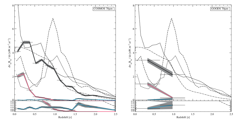
Figure 7: Differential 70 $\mu$m background brightness $d\nu_{70}B_{70}/dz$ as a function of redshift, in units of nW.m^-2.sr^-1. in the COSMOS field (left) and GOODS field (right). The lower part of the plot shows a linear zoom between 0 and 0.25 nW.m^-2.sr^-1 in order to exhibit the trend of cleaned sources and AGNs. Black solid lines: total contribution of infrared galaxies. Solid red lines: contribution from resolved sources only. Solid blue line: contribution from AGN only. Dash line Lagache et al. (2004) model, with $S_{24}>80\leavevmode\nobreak\ \mu$Jy cut. Dot line: Le Borgne et al. (2009) model, with $S_{24}>80\leavevmode\nobreak\ \mu$Jy cut. Dot-dash line:Valiante et al. (2009). Dot-dot-dot-dash line: Bethermin et al. (2010c) model, with $S_{24}>80\leavevmode\nobreak\ \mu$Jy cut. Models are discussed in Sect. 4.5 and figure 10.

3.2 Photometry and uncertainty estimations

We perform aperture photometry on the stacked images with the following parameters at 160 $\mu$m: aperture radius of 25”, a sky annulus to estimate the background between 80 and 110”, and an aperture correction of 2.29. At 70 $\mu$m, the parameters are: 18”, 50 and 70”, and 1.68. We have secure detections in all redshift bins at 160 $\mu$m and 70 $\mu$m, except in the two highest redshift bin ($z>1.3$) in GOODS. The signal to noise ratio is better in COSMOS than in GOODS, due to the larger number of sources used (the number of sources used are reported in tables 2 to 5). We thus will take into account in our analysis the redshifts bins $0<z<1.3$ in GOODS and $0<z<2.5$ in COSMOS.

The error bars come from three quadratically summed terms. 1- the photometry uncertainty. 2- the Poisson noise coming from the number of stacked sources. 3- a bootstrap analysis.

The bootstrap analysis is done by running the stacking process $N_{b}$ times (usually $N_{b}=5000$ and $N_{b}=14000$ for GOODS and COSMOS resp.) of a new sample composed of randomly selected sources from our original sample, keeping the total number of sources constant Bavouzet (2008); this means that some stacked positions might be present zero, or multiple times in each realization. The bootstrap error bar comes from the standard deviation of the distribution of the photometry measured on these $N_{b}$ realizations. Notice that the signal-to-noise ratio of the detections in the stacked images (only photometric) is higher than the value quoted in this paper, since we add the Poisson and bootstrap terms to estimate the final error bar, which takes into account the dispersion of the underlying sample. The final error bar is thus larger than just the photometric noise estimate. The error bars on the AGNs samples were determined using a smaller number of bootstrap, $N_{b}=100$ and $N_{b}=2000$ for GOODS and COSMOS respectively.

The variance due to the large scale structure (also known as cosmic variance) and field-to-field variations is a systematic component of the noise, that is difficult to estimate at this stage. The Poisson noise, used here, gives a strict lower limit of the cosmic variance.

3.3 Measurements

By adding the brightness obtained from the stacking of 24 $\mu$m sources with $S_{24}\geq 80\leavevmode\nobreak\ \mu$Jy and the few detected far-infrared sources, we measure $B_{160_{tot-GOODS}}=7.53\pm 0.52$ nW.$m^{-2}$.$sr^{-1}$ at 160 $\mu$m, $B_{70_{tot-GOODS}}=3.97\pm 0.17$ nW.$m^{-2}$.$sr^{-1}$ at 70 $\mu$m and $B_{160_{tot-COSMOS}}=7.88\pm 0.19$ nW.$m^{-2}$.$sr^{-1}$ at 160 $\mu$m, $B_{70_{tot-COSMOS}}=4.95\pm 0.08$ nW.$m^{-2}$.$sr^{-1}$ at 70 $\mu$m (see also the summary in Tab. 6).

If we compare with the models from Lagache et al. (2004), Le Borgne et al. (2009), and Bethermin et al. (2010c) (cf section 4.5 and Tab. 6) applying the same selection of using the 24 $\mu$m sources with $S_{24}\geq 80\leavevmode\nobreak\ \mu$Jy, we obtain that we resolve 66 to 89% of the 160 $\mu$m background, and 75 to 98% of the 70 $\mu$m background.

To be more specific, using the only post-Herschel model in hand Bethermin et al. (2010c), our data show that we resolve in COSMOS 90% at 160 $\mu$m and 98% at 70 $\mu$m of the background we are supposed to measure with the selection at 24 $\mu$m applied. Our selection introduces an incompleteness in the CIB estimate due to the fainter 24 $\mu$m sources ($S_{24}<80\leavevmode\nobreak\ \mu$Jy), missing in our analysis; this loss implies that we resolve 68% of the total 160 $\mu$m background and 81% of the total 70 $\mu$m background in COSMOS (see sect. 4.5 for the details). For comparison, Berta et al. (2010) identified about 50% of the 100 and 160 $\mu$m backgrounds in individual sources, and account for 50 to 75% of the background when stacking at the positions of 24 $\mu$m galaxies, as we do.

4 Discussion

In the following, we present the measurements and the models in the form of $\frac{d(\nu B_{\nu})}{dz}$ versus redshift $z$, where $\nu B_{\nu}$ is the CIB brightness in nW.m^-2.sr^-1, $\lambda$ is the wavelength (70 $\mu$m or 160 $\mu$m) and $\nu$ the corresponding frequency. This representation has the advantage of being independent of the redshift binning, thus allowing a direct comparison between datasets and models differently sampled in redshift. We discuss data and models with the prior selection of $S_{24}>80\leavevmode\nobreak\ \mu$Jy, and will show (sect. 4.5) that our conclusions for $z<1.5$, i.e. where most of the FIR background arises, are not modified by this prior selection compared to taking fainter galaxies.

4.1 The 160 $\mu$m background: history since $z=2$

The distribution of the $160\leavevmode\nobreak\ \mu$m CIB measured brightness as a function of redshift (Fig. 6) shows a plateau between redshifts 0.3 and 0.9 in COSMOS and GOODS fields, followed by a decrease at higher redshift. The small dip at $z=0.5$ in COSMOS is not significant, since it disappears when increasing the size of the redshift bin ($\Delta z=0.3$ instead of 0.15) and is likely due to a structure in the COSMOS field. The GOODS field has the same trend in redshift.

The contribution from resolved sources is maximum at $z<0.3$ and strongly decreases at higher redshift, in agreement with the identifications of Frayer et al. (2006a). The AGN contribution is rather constant with redshift; the relative contribution of AGN thus rises with redshift. Assuming the COSMOS field is representative of the whole CIB population, we derive that 33% of the 160 $\mu$m background is accounted at redshifts $0<z<0.5$, 41% for $0.5<z<1$, 17% for $1<z<1.5$, and 9% for $1.5<z<2$. Our results are consistent with Berta et al. (2010), who analyzed a deep sample in the GOODS-N field at 160 $\mu$m with PACS/Herschel. Most of the far-infrared sources are resolved by Herschel, and the stacks of 24 $\mu$m sources provide slightly more depth. Their peak at $z=1$ is more pronounced than our analysis.

The Lagache et al. (2004), Le Borgne et al. (2009),Valiante et al. (2009) and Bethermin et al. (2010c) models are overplotted to our measurements in Fig. 6, using the same selection of $S_{24}\geq 80\leavevmode\nobreak\ \mu$Jy as applied on the data. Pre-Herschel models predict different redshift distribution of $d\nu_{160}B_{160}/dz$. The Lagache et al. (2004) models peaks at $z\sim 1$, and does not fit our data. Our data are in better qualitative agreement with the Le Borgne et al. (2009) model, (except for $z<0.3$), but none models fit the $z>1$ tail. The problem of the discrepancy between our data and the Le Borgne et al. (2009) model at $z<0.3$ might be twofold: our data lacks of statistics at very low redshift due to the relative small sky area, and the model might be overpredicting low-z galaxies because of the lack of a cold component in the galaxies SED used. The Bethermin et al. (2010c) fits well the low, intermediate and high redshift ranges, likely because it is based on the minimization of recent Spitzer and Herschel data, and already takes into account the FIR and submm statistical properties of galaxies (see Sect. 4.5).

4.2 The 70 $\mu$m background: history since $z=2$

The distribution of the $70\leavevmode\nobreak\ \mu$m CIB measured brightness as a function of redshift (Fig. 7) shows a maximum contribution $z<0.5$ in COSMOS, consistent with the GOODS measurements. The peak contribution at 70 $\mu$m lies at lower redshift than at 160 $\mu$m, which is expected as a consequence of the K-correction (the effect of the redshifted shape of the galaxies spectra). This effect is also seen between 100 $\mu$m and 160 $\mu$m in the PACS/Herschel data by Berta et al. (2010). The dip at $z\sim 0.5$ is likely a cosmic variance effect, as it is not seen in the GOODS field, and it disappears when we use broader redshift bins. This dip does not change our conclusion about the 70 $\mu$m background emission with redshift.

The contribution from resolved sources is maximum at $0.15<z<0.3$ and strongly decreases at higher redshift, in agreement with the identifications of Frayer et al. (2006a). The AGN contributions is rather constant with redshift. Assuming the COSMOS field is representative of the whole CIB population, we derive that 43% of the 70 $\mu$m background is accounted at redshifts $0<z<0.5$, 38% for $0.5<z<1$, 13% for $1<z<1.5$, and 5% for $1.5<z<2$.

The Lagache et al. (2004) model predicts a peak of the CIB at 70 $\mu$m at around $z=1$, not seen in the data. The Le Borgne et al. (2009) predicts a peak at lower redshift ($z\leq 0.5$), with a strong contribution at $z\sim 0$, not seen either in the data; otherwise, the decrease at $z>0.5$ has a shape comparable to the data, despite a larger high redshift tail. The post-Herschel Bethermin et al. (2010c) model nicely follows observed evolution in COSMOS and GOODS (Fig. 7).

Figure 8: The relative contribution of identified AGN to the 70 and 160 $\mu$m CIB as a function of redshift, with the selection at 24 $\mu$m with $S_{24}>80\mu$Jy.

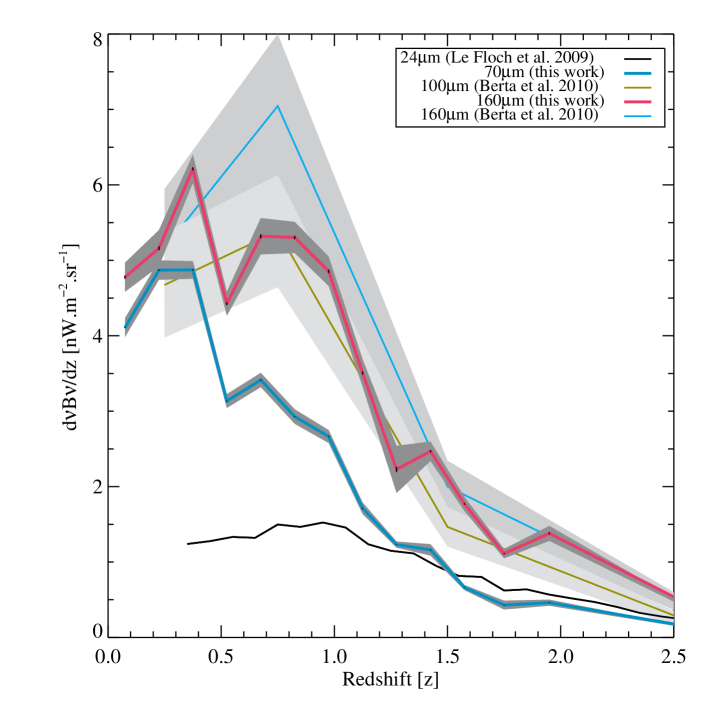
Figure 9: The Cosmic Infrared Background history since $z\sim 2$ at 24, 70, 100 and 160 $\mu$m as measured from galaxies selected at 24 $\mu$m with $S_{24}>80\mu$Jy. 24 $\mu$m data come from Le Floc’h et al. (2009), 70 and 160 $\mu$m from this work, all using the Spitzer/MIPS data of COSMOS field. 100 and 160 $\mu$m data in four redshift bins come from Berta et al. (2010) in GOODS-N with Herschel/PACS (and using the same 24 $\mu$m prior.).

4.3 Role of AGN

The AGN contribution in each redshift bin is shown on Fig. 7 and 6, as the lower blue area. The estimate of this contribution can be considered as a “best effort” estimate, because of the difficulty of the task of identifying the origin of the far-infrared emission (star formation or AGN). Our AGN identification relies on X-ray detections and IRAC colors Caputi et al. (2006); Salvato et al. (2009), but the far-infrared emission is not necessarily physically linked to the AGN Le Floc’h et al. (2007).

Our analysis shows that the absolute contribution of AGN to the CIB at 70 and 160 $\mu$m is rather constant with redshift. Figure 8 shows the relative contribution to the CIB, and is obtained by dividing the AGN contribution to the total CIB contribution. Because of the smaller contribution of higher redshift sources to the CIB, the AGN fraction contribution to the CIB is increasing with redshift, from about $3\pm 10$% for $0<z<1.5$, and up to possibly 15-25% for $z>1.5$, but our large error bars do not allow any meaningful estimate. We thus can only state that the relative AGN contribution is less than about 10% at $z<1.5$. Our results are in agreement with Daddi et al. (2007) who predict that the contribution of AGNs shouldn’t exceed more than 7$\%$ up to a redshift unity.

AGN are thought to play a central role in terms of physical processes driving galaxy evolution and regulating star formation trough feedback (Magorrian et al., 1998; Ferrarese & Merritt, 2000; Bower et al., 2006; Hopkins et al., 2006; Cattaneo et al., 2009; Hopkins et al., 2010, e.g. ). However, our work confirms that, in terms of total energy contributions to the CIB, the AGN play a minor role. This conclusion is in agreement with the identifications of Frayer et al. (2006a) and the analysis of Valiante et al. (2009), where (their figure 19) is shown that less than 10% of the sources with $S_{24}>80\leavevmode\nobreak\ \mu$Jy (Dole et al., 2006, i.e. the sources making-up the CIB at 24 to 160 $\mu$m, see ) have a significant AGN contribution.

4.4 The 24, 70, 100 and 160 $\mu$m backgrounds

The mid- and far-infrared background buildup at 24, 70, 100 and 160 $\mu$m as a function of redshift is summarized in figure 9 and is available online. The 24 $\mu$m data come from Le Floc’h et al. (2009) and were normalized to 2.86 nW.m^-2.sr^-1 Bethermin et al. (2010), and the data at 100 $\mu$m come from Berta et al. (2010), while the data at 70 and 160 $\mu$m come from this work. At wavelengths larger than 60 $\mu$m, the observed buildup sequence shows an increasing contribution from $z\sim 0.5$ to $z\sim 1$ with increasing wavelength. This behaviour is expected, as consequence of the redshifted peak in the galaxy spectral energy distributions, or k-correction (Lagache et al., 2004, 2005, e.g. ). The 24 $\mu$m buildup shows a flatter (or broader) distribution in redshift, with a maximum contribution around $z\sim 1$; This mid-infrared distribution has a relative $z>1.5$ contribution larger than in the far-IR, i.e. the decay slope is smaller at 24 $\mu$m than at 70 $\mu$m and larger wavelengths.

A detailed comparison, however, is still difficult because of the cosmic variance. The results from Berta et al. (2010) are based on GOODS-N, an area about 50 times smaller than used here. We furthermore showed that large scale structure is visible at $z<0.5$ in the COSMOS field.

The fact that most of the CIB between 100 and 160 $\mu$m is identified as being produced by $z<1$ sources is in line with expectations (Lagache et al., 2005; Bethermin et al., 2010c, e.g. ). The 24 $\mu$m background has, however, a significant fraction from galaxies at $z>1$ (Le Floc’h et al., 2009, 30%, according to ). As expected and observed Marsden et al. (2009), most of the submillimeter background is made of sources lying at higher redshifts ($z>1.5$). This wavelength versus redshift dependence of the background can be explained by the sum of SED of galaxies at various redshifts, in particular the peak emission in the far-infrared of the reprocessed starlight by dust being redshifted. Thus, the SED of the CIB is broader and flatter at far-infrared and submillimeter wavelengths than any individual galaxy SED.

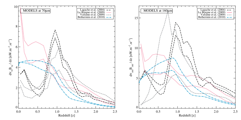
Figure 10: Differential 70 (left) and 160 $\mu$m (right) background brightness $d\nu_{\nu}B_{\nu}/dz$ as a function of redshift, in units of nW.m^-2.sr^-1, as predicted by 4 models: Dash black line: Lagache et al. (2004) model; Dot magenta line: Le Borgne et al. (2009) model; Dot-dash grey line: Valiante et al. (2009); Dot-dot-dot-dash blue line: Bethermin et al. (2010c) model. For each model, the top line corresponds to all galaxies, and the bottom line to the prior selection (used in this work) of $S_{24}>80\leavevmode\nobreak\ \mu$Jy.

4.5 The models

These observations can be confronted to models. We use three backwards evolution models developed to fit infrared data: Lagache et al. (2004), Le Borgne et al. (2009), Valiante et al. (2009), and Bethermin et al. (2010c), among an abundant literature (Franceschini et al., 2008, 2009; Pearson & Khan, 2009; Rowan-Robinson, 2009, for the most recent: ). The main feature of the Lagache et al. (2004) model is the use of two galaxy populations spectral energy distributions (SED), normal/cold and starburst galaxies, parametrized by their total infrared luminosity. The local luminosity functions are fitted, and the evolution in redshift is applied in order to fit the additional constraints of the observed number counts, CIB SED, and CIB fluctuation level. The Le Borgne et al. (2009) model is based on an automated minimization of the difference between the model and selected datasets (local luminosity functions, number counts, CIB absolute level) with a given SED library Chary et al. (2001). The Valiante et al. (2009) model introduces scatter in the SED by using Monte-Carlo runs within an extended library based on observations from the Spitzer archive, and containing starburst and AGN contributions as a function of IR luminosity. Those three models used Spitzer data, and were developed prior to the availability of Herschel data. Finally, the Bethermin et al. (2010c) model is a fully-parametric approach, automatically fitting the latest Spitzer, BLAST & Herschel data with Markov chain Monte Carlo (MCMC) Dunkley et al. (2005) method, and using the Lagache et al. (2004) SED library of two galaxy populations.

Figures 6 and 7 overplot these three models in the case of a prior selection at 24 $\mu$m (with $S_{24}>80\leavevmode\nobreak\ \mu$Jy) in order to be consistent with the data we are comparing with. Figure 10 shows the models, with this prior cut, but also without any cut, i.e. all the galaxies. The main differences can be summarized as follows:

• the Lagache et al. (2004) model predicts a contribution of infrared galaxies to the 70 and 160 $\mu$m backgrounds peaking at $z\sim 1$, which is not observed; also the predicted dip at $z\sim 0.5$ is not observed either.

• the Le Borgne et al. (2009) model overpredicts the galaxy contributions at $z\leq 0.3$, in disagreement with observations, despite the poor statistics of the observations; the origin is likely a lack of a cold galaxy component at $z\sim 0$. The general shape of the model at $z>0.3$ agrees with the data, despite predicted peak and high-redshift ($z>1$) tail slightly higher than observed.

• the Valiante et al. (2009) model has similar trends as Lagache et al. (2004): almost no contribution at low redshift (in disagreement with data at 70 and 160 $\mu$m), and a pronounced peak at $z\sim 1$, not observed. This models reproduces well, however, the $z>1$ tail at 160 $\mu$m (but not at 70 $\mu$m).

• the Bethermin et al. (2010c) model provides a better fit to the data, likely because its minimization on recent Spitzer & Herschel data Bethermin et al. (2010); Oliver et al. (2010) at far-infrared and submillimeter wavelengths already takes into account the statistical properties of galaxies in an empirical way.

• the selection of $S_{24}>80\leavevmode\nobreak\ \mu$Jy galaxies to estimate the background buildup with redshift produces an almost flat cut in redshift to the brightness (comparison of the two lines for each model in fig. 10, except for Valiante et al. (2009) at 160 $\mu$m with larger variations). Thus the peak and the structure in redshift observed with the $S_{24}>80\leavevmode\nobreak\ \mu$Jy cut is not much affected by this selection, and our conclusions based on this cut can be extended to the whole CIB buildup, at least for $z<2.5$. However, the $S_{24}>80\leavevmode\nobreak\ \mu$Jy cut might cause a problem of strong incompleteness at Herschel SPIRE wavelengths, made-up by higher-redshift sources Lagache et al. (2005); Marsden et al. (2009); A need to use fainter 24 $\mu$m flux densities is thus required at submm wavelengths.

All these models predict similar star formation rates and luminosity function evolutions. Our work put stronger constraints on the models, which will have to fine-tune either the galaxies SED used or refine the luminosity function evolutions.

5 Conclusion

As shown by Le Floc’h et al. (2009) and our results, the CIB buildup allows to break degeneracies present in the models (same predicted number counts and CIB SED, but different redshift histories for the luminosity functions for instance). Using exquisite Spitzer data on one of the widest and deepest fields, we are able to measure that the maximum contribution of the 70 $\mu$m background (as selected with 24 $\mu$m galaxies with $S_{24}>80\leavevmode\nobreak\ \mu$Jy) occurs at $z<0.5$ and at $0.3<z<0.9$ for the 160 $\mu$m background.

We measure that 74% of the 160 $\mu$m background was emitted at $z\leq 1$, and 81% at 70 $\mu$m. We also provided an estimate of the AGN contribution to the far-infrared background of less than about 10% for $z<1.5$.

The comparison with preliminary Herschel/PACS data on GOODS-N from Berta et al. (2010) is in line with our findings, despite the uncertainties due to large scale structure. The consistency of the results confirms that the stacking analysis method is a valid approach to estimate the components of the far-IR background using prior information on resolved mid-IR sources.

The Lagache et al. (2004) model predictions mainly disagree with the data, since the peak contribution at $z\sim 1$ is not observed. The Le Borgne et al. (2009) model disagrees with the data at low redshift (likely due to the SED used), but succeeds in reproducing most of the observed trend, despite an excess at $z>1.5$. The Bethermin et al. (2010c) model is favored by the data.

Our study, combined with those of Le Floc’h et al. (2009) and Berta et al. (2010), can allow to better constrain the models of galaxy evolution, since their predictions can strongly vary with redshift, despite good fits of the number counts, luminosity functions and cosmic infrared background spectral energy distribution.

This study, together with forthcoming works to be done on Herschel data, will also help refining the models to compute the far-infrared and submillimeter emissivity with redshift, needed to compute the optical depth for (hundreds of) TeV photons. Since the opacity of the Universe for TeV photons depends on the infrared luminosity density along the line of sight, the buildup history of the CIB has direct effect on the TeV photons propagation. We showed that most ($\sim$80%) of the far-infrared background is produced at $z<1$, in a regime where many blazars are observed (Aharonian et al., 2006; Albert & Magic Collaboration, 2008, e.g. ). The model predictions for TeV obscuration models (Mazin & Raue, 2007; Franceschini et al., 2008; Stecker & Scully, 2009; Kneiske & Dole, 2010; Younger & Hopkins, 2010; Bethermin et al., 2010c, e.g. ) could be disentangled at $z\leq 0.3$, where the CIB impacts high energy photons the most, by comparing their CIB buildup history with our data.

Table 2: The CIB brightness by redshift range at 160 $\mu$m, in units of nW.$m^{-2}$.$sr^{-1}$, in the case of the GOODS fields. The subscript “stack” refers to the measurement of the signal on the cleaned and stacked image; “sources” to the individually detected sources; “AGN” to the sources identified as AGN by Caputi et al. (2006). The total number of sources used in this analysis is thus $N_{stack}+N_{sources}$.

	0$<$ $z$ $<$0.65	0.65$<$ $z$ $<$1.3	1.3$<$ $z$ $<$2	$z$ $>$2
$N_{stack}$	317	573	258	198
$N_{sources}$	10	11	3	2
$N_{AGNs}$	9	45	38	44
$B_{160_{stack}}$	2.18 $\pm$ 0.45	2.39 $\pm$ 0.54	1.13 $\pm$ 0.35	0.78 $\pm$ 0.27
$B_{160_{sources}}$	0.57 $\pm$ 0.18	0.34 $\pm$ 0.11	0.06 $\pm$ 0.04	0.07 $\pm$ 0.05
$B_{160_{AGNs}}$	0.04 $\pm$ 0.07	0.17 $\pm$ 0.25	0.32 $\pm$ 0.22	0.20 $\pm$ 0.19
$B_{160_{tot}}$	2.75 $\pm$ 0.46	2.73 $\pm$ 0.54	1.19 $\pm$ 0.35	0.85 $\pm$ 0.27

Table 3: The CIB brightness by redshift range at 70 $\mu$m, in units of nW.$m^{-2}$.$sr^{-1}$, in the GOODS fields. Terms are defined in the caption of Tab. 2.

	0$<$ $z$ $<$0.65	0.65$<$ $z$ $<$1.3	1.3$<$ $z$ $<$2	$z$ $>$2
$N_{stack}$	317	575	259	198
$N_{sources}$	19	5	1	0
$N_{AGNs}$	9	45	38	44
$B_{70_{stack}}$	1.29 $\pm$ 0.22	1.25 $\pm$ 0.28	0.35 $\pm$ 0.15	0.15 $\pm$ 0.12
$B_{70_{sources}}$	0.77 $\pm$ 0.18	0.14 $\pm$ 0.07	0.01 $\pm$ 0.015	–
$B_{70_{AGNs}}$	0.05 $\pm$ 0.03	0.1 $\pm$ 0.12	0.11 $\pm$ 0.08	0.11 $\pm$ 0.12
$B_{70_{tot}}$	2.06 $\pm$ 0.24	1.4 $\pm$ 0.28	0.36 $\pm$ 0.15	0.15 $\pm$ 0.12

Table 4: The CIB brightness by redshift range at 160 $\mu$m, in units of nW.$m^{-2}$.$sr^{-1}$, in the case of the COSMOS field. The subscript “stack” refers to the measurement of the signal on the cleaned and stacked image; “sources” to the individually detected sources; “AGN” to the sources identified as AGN by Salvato et al. (2009). The total number of sources used in this analysis is thus $N_{stack}+N_{sources}$.

	0$<$ $z$ $<$0.15	0.15$<$ $z$ $<$0.3	0.3$<$ $z$ $<$0.45	0.45$<$ $z$ $<$0.6	0.6$<$ $z$ $<$0.75	0.75$<$ $z$ $<$0.9	0.9$<$ $z$ $<$1.05
$N_{stack}$	2083	1559	2853	2201	3225	3590	3478
$N_{sources}$	56	40	18	9	11	12	6
$N_{AGNs}$	34	32	74	48	88	109	123
$B_{160_{stack}}$	0.43 $\pm$ 0.04	0.56 $\pm$ 0.04	0.87 $\pm$ 0.05	0.63 $\pm$ 0.04	0.76 $\pm$ 0.07	0.75 $\pm$ 0.06	0.71 $\pm$ 0.06
$B_{160_{sources}}$	0.3 $\pm$ 0.001	0.21 $\pm$ 0.002	0.07 $\pm$ 0.001	0.03 $\pm$ 0.001	0.034 $\pm$ 0.001	0.043 $\pm$ 0.001	0.021 $\pm$ 0.001
$B_{160_{AGNs}}$	0.02 $\pm$ 0.006	0.01 $\pm$ 0.005	0.03 $\pm$ 0.01	0.02 $\pm$ 0.01	0.02 $\pm$ 0.01	0.01 $\pm$ 0.01	0.02 $\pm$ 0.01
$B_{160_{tot}}$	0.72 $\pm$ 0.04	0.77 $\pm$ 0.04	0.93 $\pm$ 0.05	0.66 $\pm$ 0.04	0.8 $\pm$ 0.07	0.8 $\pm$ 0.06	0.73 $\pm$ 0.06
	1.05$<$ $z$ $<$1.2	1.2$<$ $z$ $<$ 1.35	1.35$<$ $z$ $<$1.5	1.5$<$ $z$ $<$1.65	1.65$<$ $z$ $<$1.85	1.85$<$ $z$ $<$2.05	$z$ $>$2.05
$N_{stack}$	2670	1401	2044	1311	1519	2073	2833
$N_{sources}$	2	0	2	2	0	1	2
$N_{AGNs}$	83	76	55	225	230	198	288
$B_{160_{stack}}$	0.52 $\pm$ 0.05	0.33 $\pm$ 0.09	0.36 $\pm$ 0.04	0.26 $\pm$ 0.03	0.22 $\pm$ 0.02	0.27 $\pm$ 0.04	0.47 $\pm$ 0.04
$B_{160_{sources}}$	0.005 $\pm$ 0.0003	–	0.006 $\pm$ 0.0003	0.006 $\pm$ 0.0003	–	0.003 $\pm$ 0.0001	0.007 $\pm$ 0.0003
$B_{160_{AGNs}}$	0.02 $\pm$ 0.01	0.02 $\pm$ 0.01	0.01 $\pm$ 0.008	0.04 $\pm$ 0.03	0.04 $\pm$ 0.03	0.05 $\pm$ 0.03	0.04 $\pm$ 0.03
$B_{160_{tot}}$	0.53 $\pm$ 0.05	0.33 $\pm$ 0.09	0.37 $\pm$ 0.04	0.27 $\pm$ 0.03	0.22 $\pm$ 0.02	0.28 $\pm$ 0.04	0.47 $\pm$ 0.04

Table 5: The CIB brightness by redshift range at 70 $\mu$m, in units of nW.$m^{-2}$.$sr^{-1}$ , in the COSMOS field. Terms are defined in the caption of Tab. 4.

	0$<$ $z$ $<$0.15	0.15$<$ $z$ $<$0.3	0.3$<$ $z$ $<$0.45	0.45$<$ $z$ $<$0.6	0.6$<$ $z$ $<$0.75	0.75$<$ $z$ $<$0.9	0.9$<$ $z$ $<$1.05
$N_{stack}$	2083	1559	2853	2202	3225	3590	3478
$N_{sources}$	77	82	48	23	13	11	3
$N_{AGNs}$	34	32	74	48	88	110	123
$B_{70_{stack}}$	0.31 $\pm$ 0.03	0.39 $\pm$ 0.02	0.6 $\pm$ 0.03	0.42 $\pm$ 0.03	0.47 $\pm$ 0.03	0.41 $\pm$ 0.03	0.39 $\pm$ 0.03
$B_{70_{sources}}$	0.31 $\pm$ 0.001	0.34 $\pm$ 0.001	0.13 $\pm$ 0.0005	0.05 $\pm$ 0.0003	0.04 $\pm$ 0.0003	0.027 $\pm$ 0.0003	0.008 $\pm$ 0.0001
$B_{70_{AGNs}}$	0.011 $\pm$ 0.004	0.008 $\pm$ 0.003	0.015 $\pm$ 0.006	0.009 $\pm$ 0.003	0.016 $\pm$ 0.005	0.015 $\pm$ 0.007	0.015 $\pm$ 0.008
$B_{70_{tot}}$	0.62 $\pm$ 0.03	0.73 $\pm$ 0.02	0.73 $\pm$ 0.03	0.47 $\pm$ 0.03	0.51 $\pm$ 0.03	0.44 $\pm$ 0.03	0.4 $\pm$ 0.03
	1.05$<$ $z$ $<$1.2	1.2$<$ $z$ $<$ 1.35	1.35$<$ $z$ $<$1.5	1.5$<$ $z$ $<$1.65	1.65$<$ $z$ $<$1.85	1.85$<$ $z$ $<$2.05	$z$ $>$2.05
$N_{stack}$	2670	1401	2044	1311	1519	2073	2833
$N_{sources}$	2	1	2	0	0	0	0
$N_{AGNs}$	83	76	55	225	232	200	288
$B_{70_{stack}}$	0.25 $\pm$ 0.02	0.18 $\pm$ 0.01	0.17 $\pm$ 0.02	0.1 $\pm$ 0.01	0.09 $\pm$ 0.02	0.09 $\pm$ 0.02	0.16 $\pm$ 0.02
$B_{70_{sources}}$	0.004 $\pm$ 0.0001	0.002 $\pm$ 0.0001	0.003 $\pm$ 0.0001	–	–	–	–
$B_{70_{AGNs}}$	0.14 $\pm$ 0.007	0.011 $\pm$ 0.005	0.006 $\pm$ 0.004	0.28 $\pm$ 0.012	0.026 $\pm$ 0.015	0.022 $\pm$ 0.01	0.029 $\pm$ 0.018
$B_{70_{tot}}$	0.26 $\pm$ 0.02	0.18 $\pm$ 0.01	0.17 $\pm$ 0.02	0.1 $\pm$ 0.01	0.09 $\pm$ 0.2	0.09 $\pm$ 0.02	0.15 $\pm$ 0.02

Table 6: The total CIB brightness at 160 $\mu$m & 70$\mu$m for the GOODS & COSMOS fields, in units of nW.$m^{-2}$.$sr^{-1}$: lines 1 & 2: our estimates; line 3: Bethermin et al. (2010) CIB measured value using number counts integration; line 4: Bethermin et al. (2010) CIB value with extrapolation of the number counts in power-law; line 5: Lagache et al. (2004) CIB model value with the constraint: $S_{24}$ $>$ 80 $\mu$Jy; line 6: Lagache et al. (2004) CIB model value of the total background; line 7: Le Borgne et al. (2009) CIB model value with the constraint: $S_{24}$ $>$ 80 $\mu$Jy; line 8: Le Borgne et al. (2009) CIB model value of the total background; line 9: Valiante et al. (2009) CIB model value with the constraint: $S_{24}$ $>$ 80 $\mu$Jy; line 10: Valiante et al. (2009) CIB model value of the total background; line 11: Bethermin et al. (2010c) CIB model value with the constraint: $S_{24}$ $>$ 80 $\mu$Jy; line 12: Bethermin et al. (2010c) CIB model value of the total background.

	160 $\mu$m	70 $\mu$m
$B_{tot-GOODS}$	7.53 $\pm$ 0.84	3.97 $\pm$ 0.41
$B_{tot-COSMOS}$	7.88 $\pm$ 0.19	4.95 $\pm$ 0.08
$B_{Bethermin}$	9.0 $\pm$ 1.1	5.2 $\pm$ 0.4
$B_{Bethermin_{CIBestimate}}$	$14.6^{+7.1}_{-2.9}$	$6.4^{+0.7}_{-0.6}$
$B_{model_{Lagache}}(S_{24}>80\mu Jy)$	11.91	5.73
$B_{model_{Lagache}}$	14.87	6.78
$B_{model_{LeBorgne}}(S_{24}>80\mu Jy)$	9.54	6.65
$B_{model_{LeBorgne}}$	13.57	8.54
$B_{model_{Valiante}}(S_{24}>80\mu Jy)$	6.84	4.27
$B_{model_{Valiante}}$	16.70	6.98
$B_{model_{Bethermin}}(S_{24}>80\mu Jy)$	8.82	5.02
$B_{model_{Bethermin}}$	11.66	6.09

References

- (1)
- Aharonian et al. (2006) Aharonian, F, Akhperjanian, A. G, Bazer-Bachi, A. R, Beilicke, M, Benbow, W, et al., 2006, Nature, 440:1018.
- Aharonian et al. (2007) Aharonian, F, Akhperjanian, A. G, Barres De Almeida, U, Bazer-Bachi, A. R, Behera, B, Beilicke, M, Benbow, W, et al., 2007, A&A, 475:L9–L13.
- Albert & Magic Collaboration (2008) Albert, J & Magic Collaboration. 2008, Science, 320:1752.
- Alonso-Herrero et al. (2006) Alonso-Herrero, A, Perez-Gonzalez, P. G, Alexander, D. M, Rieke, G. H, Rigopoulou, D, Le Floc’h, et al., 2006, ApJ, 640:167.
- Bavouzet (2008) Bavouzet, N. Les galaxies infrarouges: distribution spectrale d’énergie et contributions au fond extragalactique. PhD thesis, Université Paris-Sud 11 http://tel.archives-ouvertes.fr/tel-00363975/, 2008.
- Berta et al. (2010) Berta, S, Magnelli, B, Lutz, D, Altieri, B, Aussel, H, arXiv:1005.1073, 2010.
- Bethermin et al. (2010) Bethermin, M, Dole, H, Beelen, A, & Aussel, H. et al., 2010, A&A, 512:78.
- Bethermin et al. (2010b) Bethermin, M, Dole, H, Cousin, M, & Bavouzet, N. 2010, A&A, 516, 43
- Bethermin et al. (2010c) Bethermin, M, Dole, H, Lagache, G, Le Borgne, D., & Penin, A. 2010, A&A, in prep
- Bower et al. (2006) Bower, R G, Benson, A J, Malbon, R, Helly, J C, Frenk, C S, et al., 2006, MNRAS, 370:645.
- Brusa et al. (2007) Brusa, M, Zamorani, G, Comastri, A, Hasinger, G, Cappelluti, N, et al., 2007, Astrophys. J. Suppl. Ser., 172:353–367.
- Brusa et al. (2010) Brusa, M, Civano, F, Comastri, A, Miyaji, T, Salvato, M, et al., arXiv:1004.2790, 2010.
- Cappelluti et al. (2007) Cappelluti, N, Hasinger, G, Brusa, M, Comastri, A, Zamorani, G, et al., 2007, Astrophys. J. Suppl. Ser., 172:341–352.
- Cappelluti et al. (2009) Cappelluti, N, Brusa, M, Hasinger, G, Comastri, A, Zamorani, G, et al., 2009, A&A, 497:635–648.
- Caputi et al. (2006) Caputi, K. I, Dole, H, Lagache, G, McLure, R. J, Puget, J. L, Rieke, G. H, Dunlop, J. S, Floc’h, E. L, Papovich, C, & Perez-Gonzalez, P. G. 2006, ApJ, 637:727.
- Caputi et al. (2007) Caputi, K. I, Lagache, G, Yan, L, Dole, H, Bavouzet, N, Le Floc’H, E, Choi, P. I, Helou, G, & Reddy, N. 2007, ApJ, 660:97–116.
- Cattaneo et al. (2009) Cattaneo, A, Faber, S, Binney, J, Dekel, A, Kormendy, J, et al., 2009, Nature, 460:213.
- Chary et al. (2001) Chary, R, Elbaz, D. 2001, ApJ, 556, 562
- Chary et al. (2004) Chary, R, Casertano, S, Dickinson, M. E, Ferguson, H. C, Eisenhardt, P. R. M, Elbaz, D, Grogin, N. A, Moustakas, L. A, Reach, W. T, & Yan, H. 2004, Astrophys. J. Suppl. Ser., 154:80.
- Clements et al. (2010) Clements, D. L, Rigby, E, Maddox, S, Dunne, L, Mortier, A, et al., arXiv:1005.2409, 2010.
- Daddi et al. (2007) Daddi, E, Alexander, D. M, Dickinson, M, Gilli, R, Renzini, A, et al., 2007, ApJ, 670:173–189.
- Dole et al. (2004) Dole, H, Floc’h, E. L, Perez-Gonzalez, P. G, Papovich, C, Egami, E, et al., 2004, Astrophys. J. Suppl. Ser., 154:87.
- Dole et al. (2006) Dole, H, Lagache, G, Puget, J. L, Caputi, K. I, Fernández-Conde, N, et al., 2006, A&A, 451:417.
- Dunkley et al. (2005) Dunkley, J, Bucher, M, Ferreira, P. G., Moodley, K., Skordis, C, 2005, MNRAS, 356:925
- Dye et al. (2010) Dye, S, Dunne, L, Eales, S, Smith, D. J. B, Amblard, A, et al., arXiv:1005.2411, 2010.
- Fernandez-Conde et al. (2008) Fernandez-Conde, N, Lagache, G, Puget, J. L, & Dole, H. 2008, A&A, 481:885–895.
- Fernandez-Conde et al. (2010) Fernandez-Conde, N, Lagache, G, Puget, J. L, & Dole, H. arXiv:1004.0123, 2010.
- Ferrarese & Merritt (2000) Ferrarese, L, Merritt, D, 2000, ApJ, 539:L9.
- Franceschini et al. (2008) Franceschini, A, G, Rodighiero, M, Vaccari, et al. 2008, A&A, 487, 837
- Franceschini et al. (2009) Franceschini, A., et al. 2009, arXiv:0906.4264
- Frayer et al. (2006a) Frayer, D. T, Fadda, D, Yan, L, Marleau, F. R, Choi, P. I, et al., 2006a, AJ, 131:250.
- Frayer et al. (2006b) Frayer, D. T, Huynh, M. T, Chary, R, Dickinson, M, Elbaz, D, et al., 2006b, ApJ, 647:L9–L12.
- Frayer et al. (2009) Frayer, D. T, Sanders, D. B, Surace, J. A, Aussel, H, Salvato, M, et al., 2009, AJ, 138:1261.
- Hauser & Dwek (2001) Hauser, M. G & Dwek, E. 2001, ARA&A, 37:249.
- Hauser et al. (1998) Hauser, M. G, Arendt, R. G, Kelsall, T, Dwek, E, Odegard, N, et al., 1998, ApJ, 508:25.
- Hogbom (1974) Hogbom, J. A., 1974, Astrophys. J. Suppl. Ser., 15:417.
- Hopkins et al. (2006) Hopkins, P. F., Hernquist, L, Cox, T J, Di Matteo, T, Robertson, B, Springel, V 2006, Astrophys. J. Suppl. Ser., 163:1.
- Hopkins et al. (2010) Hopkins, P. F., Younger, J D, Hayward C C, Narayanan, D, Hernquist, L 2010, MNRAS, 402:1693.
- Ilbert et al. (2009) Ilbert, O, Capak, P, Salvato, M, Aussel, H, McCracken, H. J, et al.,xs 2009, ApJ, 690:1236.
- Kashlinsky (2005) Kashlinsky, A. 2005, Phys. Rep., 409:361.
- Kneiske & Dole (2009) Kneiske, T. M & Dole, H. 2009, A&A.
- Kneiske & Dole (2010) Kneiske, T & Dole, H. 2010, A&A, in press, ArXiv:1001.2132.
- Lagache et al. (2004) Lagache, G, Dole, H, Puget, J. L, Perez-Gonzalez, P. G, Floc’h, E. L, Rieke, G. H, Papovich, C, Egami, E, Alonso-Herrero, A, Engelbracht, C. W, Gordon, K. D, Misselt, K. A, & Morrison, J. E. 2004, Astrophys. J. Suppl. Ser., 154:112.
- Lagache et al. (2005) Lagache, G, Puget, J. L, & Dole, H. 2005, ARA&A, 43:727.
- Le Borgne et al. (2009) Le Borgne, D, Elbaz, D, Ocvirk, P, & Pichon, C. 2009, A&A, 504:727–740.
- Le Floc’h et al. (2005) Le Floc’h, E, Papovich, C, Dole, H, Bell, E. F, Lagache, et al., 2005, ApJ, 632:169.
- Le Floc’h et al. (2007) Le Floc’h, E, Willmer, C. N. A, Noeske, K, Konidaris, N. P, Laird, E. S, et al., 2007, ApJ, 660, L65-L68
- Le Floc’h et al. (2009) Le Floc’h, E, Aussel, H, Ilbert, O, Riguccini, L, Frayer, D. T, et al., 2009, ApJ, 703:222.
- Magnelli et al. (2009) Magnelli, B, Elbaz, D, Chary, R. R, Dickinson, M, Le Borgne, D, Frayer, D. T, & Willmer, C. N. A. 2009, A&A, 496:57–75.
- Magorrian et al. (1998) Magorrian, J, Tremaine, S, Richstone, D, Bender, R, Bower, G, et al., 1998, AJ, 115:2285.
- Marsden et al. (2009) Marsden, G, Ade, P, Bock, J, Chapin, E, Devlin, M, et al., 2009, ApJ, 707, 1729
- Mazin & Raue (2007) Mazin, D & Raue, M. 2007, A&A, 471:439–452.
- Oliver et al. (2010) OLiver, S et al., arXiv:1005.2184
- Papovich et al. (2004) Papovich, C, Dole, H, Egami, E, Floc’h, E. L, Perez-Gonzalez, P. G, et al., 2004, Astrophys. J. Suppl. Ser., 154:70.
- Pearson & Khan (2009) C. Pearson; S. A. Khan 2009, MNRAS, 399, L11
- Puget et al. (1996) Puget, J. L, Abergel, A, Bernard, J. P, Boulanger, F, Burton, W. B, Désert, F. X, & Hartmann, D. 1996, A&A, 308:L5.
- Raue et al. (2009) Raue, M, Kneiske, T, & Mazin, D. 2009, A&A, 498:25–35.
- Rieke et al. (2004) Rieke, G. H, Young, E. T, Engelbracht, C. W, Kelly, D. M, Low, F. J, et al., 2004, Astrophys. J. Suppl. Ser., 154:25.
- Rowan-Robinson (2009) M. Rowan-Robinson 2009, MNRAS, 394, 117-123
- Salvato et al. (2009) Salvato, M, Hasinger, G, Ilbert, O, Zamorani, G, Brusa, M, et al., 2009, ApJ, 690:1250.
- Soifer & Neugebauer (1991) Soifer, B. T & Neugebauer, G. 1991, AJ, 101:354.
- Stecker & Scully (2009) Stecker, F. W & Scully, S. T. 2009, ApJ, 691:L91–L94.
- Takeuchi et al. (2006) Takeuchi, T. T, Ishii, T. T, Dole, H, Dennefeld, M, Lagache, G, & Puget, J. L. 2006, A&A, 448:525.
- Valiante et al. (2009) Valiante, E, Lutz, D, Sturm, E, Genzel, R, & Chapin, E. L. 2009, ApJ, 701:1814.
- Werner et al. (2004) Werner, M. W, Roellig, T. L, Low, F. J, Rieke, G. H, Rieke, M, et al., 2004, Astrophys. J. Suppl. Ser., 154:1.
- Younger & Hopkins (2010) Younger, J. D & Hopkins, P. F. A physical model for the origin of the diffuse cosmic infrared background. arXiv:1003.4733, 2010.