The Formation of a Magnetic Channel by the Emergence of Current-carrying Magnetic Fields

Abstract

A magnetic channel – a series of polarity reversals separating elongated flux threads with opposite polarities – may be a manifestation of a highly non-potential magnetic configuration in active regions. To understand its formation we have carried out a detailed analysis of the magnetic channel in AR 10930 using data taken by the Solar Optical Telescope /Hinode. As a result, we found upflows ($-0.5$ to $-1.0$ km s^-1) and downflows ($+1.5$ to $+2.0$ km s^-1) inside and at both tips of the thread respectively, and a pair of strong vertical currents of opposite polarity along the channel. Moreover, our analysis of the nonlinear force-free fields constructed from the photospheric magnetic field indicates that the current density in the lower corona may have gradually increased as a result of the continuous emergence of the highly sheared flux along the channel. With these results, we suggest that the magnetic channel originates from the emergence of the twisted flux tube that has formed below the surface before the emergence.

1 Introduction

Flares usually occur in regions of highly non-potential magnetic field that can contain large amount of free magnetic energy (Wang et al., 1996; Schrijver, 2009). The degree of magnetic non-potentiality has been empirically measured by different kinds of observational parameters such as magnetic gradient across the polarity inversion lines (PIL) (Wang, 2006), magnetic shear at PILs (Hagyard et al., 1984, 1990) and flux emergence at the flaring site (Ishii et al., 1998; Schrijver, 2009). Most of highly non-potential magnetic fields have complex configurations.

Zirin & Wang (1993) observed a complex magnetic field configuration called magnetic channel in an active $\delta$-type sunspot group that produced major flares. From the vector videomagnetograms taken at the Big Bear Solar Observatory, they found a series of alternating opposite polarities near the main PIL of the active region where major flares occurred about one day after. Those elongated opposite polarities were separated by channels along which the strong transverse magnetic fields were detected. Even though they did not show the direct connection between the magnetic channel and the flare occurrence, the appearance of such a sheared structure at the flaring region itself is interesting in the viewpoint of the magnetic non-potentiality of the flaring region.

The characteristics of a magnetic channel were recently studied by Wang et al. (2008) with data from the Solar Optical Telescope (SOT)/Hinode. This channel was observed between two spots of opposite polarity in AR 10930. By analyzing both vector magnetograms and three-dimensional coronal field obtained from the nonlinear force-free field (NLFFF) extrapolation, they quantified magnetic properties of the channel and confirmed that the channel was a highly sheared and non-potential structure. For instance, they measured the distribution of shear angles in the channel area using vector magnetograms and showed that the median value was 63^∘.9. They also suggested a schematic model to explain the formation mechanism of the channel. According to this model, a series of small bipoles become squeezed and elongated once they emerge because of the compactness of the background field, leading to the formation of the magnetic channel. Unfortunately, however, since they analyzed only a snapshot vector magnetogram, the study was not sufficient to show the formation process of the magnetic channel. Their analysis focused on the single set of magnetic data taken at 14 UT on December 13 when the magnetic channel was already well developed.

We aim to systematically investigate the formation process of the channel structure in AR 10930. Since a time sequential Spectropolarimeter (SP) data from SOT are available at the early phase of the channel formation, more detailed analysis could be performed at this time period. As Wang et al. (2008) mentioned, the channel is likely to have been formed due to flux emergence at the flaring region. Note that the flux emergence has been regarded as one of the important processes that increase the magnetic non-potentiality (Kurokawa, 1987; Tanaka, 1991; Ishii et al., 1998; Kurokawa et al., 2002; Brooks et al., 2003; Schrijver, 2009). In addition, it seems that the formation of the magnetic channel could be related to the flare that occurred one day later, on December 13. If we investigate how such a sheared structure developed prior to the flare occurrence, we will be able to better understand how free magnetic energy was accumulated and how the destabilization of the magnetic field took place in AR 10930. Like the active region studied by Zirin & Wang (1993), AR 10930 also shows the $\delta$-configuration and produced a number of flares including three X-class ones during its first disk passage. Due to its high degree of activity, specifically the X-class flare on 2006 December 13, many flare-related studies have been performed with AR 10930 using data from SOT/Hinode (Kubo et al., 2007; Guo & Ding, 2008; Schrijver et al., 2008; Magara & Tsuneta, 2008).

Specifically, we examine the temporal evolution of the photospheric vector magnetic fields around the formation site of the channel. We also probe the three-dimensional structures of both magnetic field and electric current in the corona above the magnetic channel by applying the NLFFF extrapolation.

The content of this paper is organized as follows. In Section 2, we describe the data and the analysis methods. Then the observational findings and their significance are presented in Section 3 that is divided into two parts. In Section 3.1, the photospheric evolution of the channel structure examined by analyzing Filtergraph (FG) and SP data is presented. The description of the temporal change in the Doppler velocity and the vector magnetic field is also included. In Section 3.2, the characteristics of the coronal magnetic field and the coronal current density deduced from the NLFFF extrapolation are presented. Finally, we summarize the key results and discuss their physical implications in Section 4.

2 Observations and Data Analysis

2.1 Data description

AR 10930 was observed from 2006 December 5 to 17 in the southern hemisphere near the solar equator. This active region is one of the highly flare-productive active regions well observed by Hinode, the Japanese satellite launched on 2006 September 22. It showed a significant rotation of sunspots during its first disk passage (Min & Chae, 2009), and several flares occurred meanwhile including the X-3.4 flare of 2006 December 13. Figure 1 shows the line-of-sight (LOS) magnetogram obtained from SP data using the center-of-gravity (COG) method (Rees & Semel, 1979; Uitenbroek, 2003; Chae et al., 2007). The COG method could be a good choice when interested in the LOS component of magnetic field only, since it takes shorter inversion time and does not require any radiative transfer model. The data were taken about 1.5 days before the X-3.4 flare. Between the two spots of opposite polarity, there are several faint threads elongated in the east-west direction. In specific, the thin structure of negative polarity indicated by the arrow is the object of our main interest. We investigate its formation and temporal evolution for about one day.

The SOT on board Hinode provides SP data that consist of full Stokes profiles of the two Fe lines at 6301.5 and 6302.5 Å taken using the slit of 0.16″ by 164″. We have examined 7 sets of SP data that were taken during the period of our interest from 17 UT on December 11 to 20 UT on the 12th. Every set covered the same field of view of about 280″ by 160″, which is large enough to cover the entire active region. One set was taken with the normal mode at 11 UT on December 12, which is characterized by the high spatial sampling of 0.16″, and a long scan time of about 160 minutes. The others were taken with the fast mode, with a coarser spatial sampling of 0.32″ and the shorter scan time of about 60 minutes. Although the coarser spatial sampling of the fast-mode scan costs the spatial resolution, its shorter scan time makes it proper for this study considering the fast change of the channel structure. The SOT also produced Stokes $I$ and $V$ filtergrams (FG) with a higher time cadence of a few minutes. These data were useful in the study of the morphological change of magnetic structures.

2.2 Data analysis

In order to measure the LOS velocity of the active region, we have applied the COG method to Stokes $I$ profiles at all the pixels in the channel site. The COG wavelength of the averaged $I$ profile of the quiet Sun was taken as the reference. It has been demonstrated by Uitenbroek (2003) that the COG method accurately derives the LOS velocity even in the case of asymmetric lines. This property makes it suitable to apply the method to our analysis since a number of the line profiles in the region of our interest near the PIL are found to be asymmetric probably because of the complexity of magnetic and velocity structures there.

The vector magnetic fields were retrieved by using the conventional Stokes inversion method that fits the observed line profiles assuming the Milne–Eddington (ME) atmosphere. The $180^{\circ}$ ambiguity was resolved by applying the Uniform Shear Method (USM) introduced by Moon et al. (2003). These authors showed that the method successfully removed the spatial discontinuities of the transverse fields of active regions containing highly sheared regions. Moon et al. (2007) also adopted USM in resolving the azimuth ambiguity of AR 10930, the same active region as the one we are studying, and showed that the method successfully worked on all areas.

After correcting the projection effect, the small part of the active region that contains the channel structure of our interest was chosen from each of vector magnetograms for the bottom boundary condition of the NLFFF extrapolation. In the optimization code devised by Wiegelmann (2004), the lateral and the top boundaries are assumed to be potential field. If the boundaries are far from the active region, the effect of the lateral boundaries on the extrapolated field could be negligible. In our case, the solid rectangle in Figure 1 shows the FOV for the NLFFF extrapolation. The magnetic structure of our interest is relatively small and far from lateral boundaries, so that field lines of this structure are likely to be closed within the computational box. Therefore, we expect that the effect of the lateral boundary condition on the computed fields would not be significant. Since the magnetic channel is fine-scale, we maintained the original spatial sampling of 0″.32 for the extrapolation. Instead, we limited the FOV for the extrapolation to about 50″ by 50″ to reduce both the computational time and the size of data.

Before the NLFFF extrapolation, all data were preprocessed following the procedure developed by Wiegelmann & Inhester (2006) in order to make the photospheric magnetic field close to force-free. Preprocessing alters the vector magnetic field so that the bottom boundary satisfies the force-free and torque-free condition (Wiegelmann & Inhester, 2006) and also represents the chromospheric force-free condition better (Jing et al., 2009). Figure 2 shows vector magnetograms before and after the preprocessing. Although fine-scale structures have been smoothed and their boundaries have been broadened after preprocessing, the channel structure is still well recognized. The directions and strength of transverse fields have also been slightly altered. The direction of transverse fields changed to be less parallel to the neutral line of the channel structure indicating that the magnetic shear in the channel region may have been reduced after preprocessing. The relatively large change of transverse fields near the negative umbral region may be due to the boundary effect. Since this region is over 15 Mm away from the channel structure, it is expected that magnetic fields with lower heights, roughly half of 15 Mm, may not be affected significantly by the boundary effect.

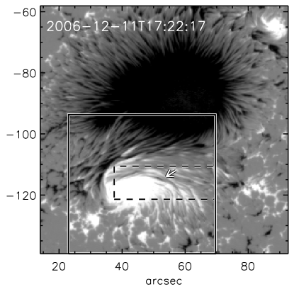
Figure 1: LOS magnetogram of AR 10930. The arrow indicates the location of the negative flux thread which is our object of interest. The solid rectangle represents the FOV for both the preprocessing and the NLFFF extrapolation, and the dashed rectangle indicates the region that we cut for the image display in Figures 4, 5, 6, and 7.

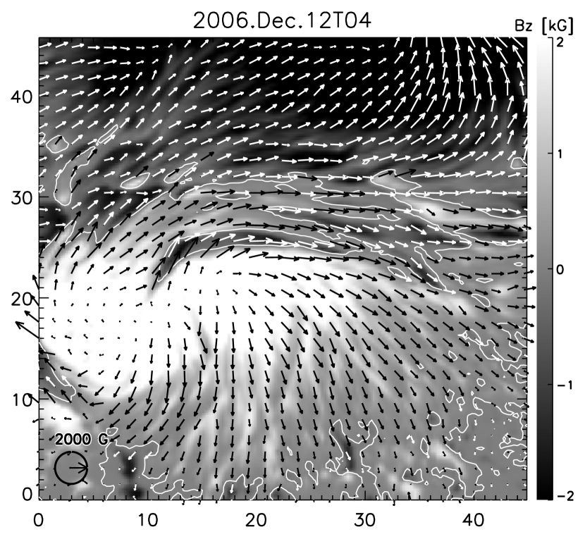
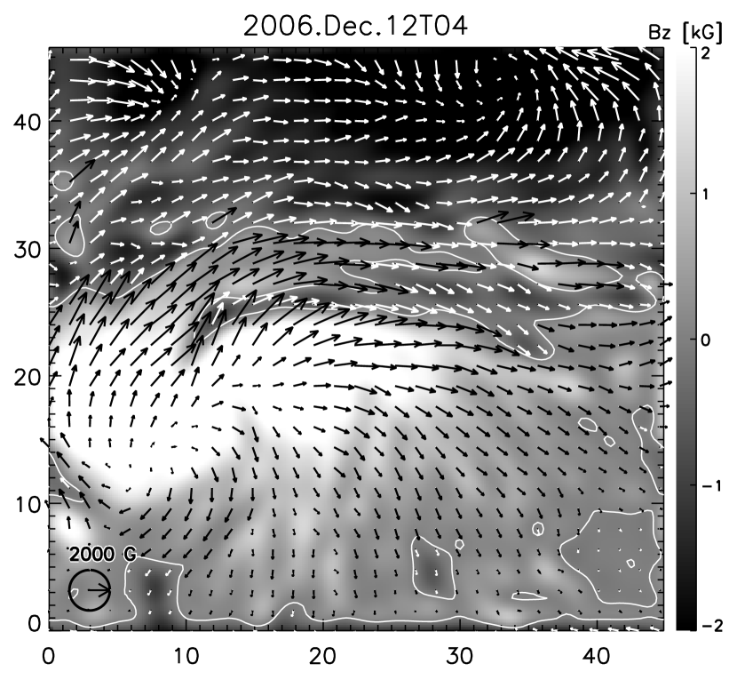
Figure 2: Vector magnetograms of AR 10930 without preprocessing (left) and with preprocessing (right).

3 Results

3.1 Photospheric magnetic and velocity fields

Figure 3 presents the time series of FG $V/I$ and $I$ maps showing the process of the formation and evolution of the magnetic channel. The most notable in the $V/I$ maps is the gradual appearance and the fast growth of a thread-like structure at the edge of the positive spot near the main PIL. As shall be shown later in this section, this process of appearance and growth physically represents the emergence of magnetic flux from below. The formation stage of this structure is well recorded in the three magnetograms taken on December 11. The first magnetogram taken at 17:27 UT on December 11 just before the formation of the channel shows that the region is dominated by the magnetic field of positive polarity with a strength of about 3000 G. However, at the elongated area pointed by an arrow, the magnetic field is weak with a strength of a few hundreds of Gauss only. This is the very location where the negative flux thread is to appear. At 20:24 UT on December 11, the polarity of the magnetic field in the area changes to negative and the thread becomes clearly visible on the surface. Although it represents the very early phase of emergence, the shape of the negative flux is quite elongated in contrast to the usual emergence of a bipole.

This negative flux thread seen in magnetograms corresponds to a dark penumbral filament in $I$ maps. This penumbral filament can be identified at the elongated area of weak field even at 17:27 UT on the 11th, before the appearance of the negative flux thread. It gets longer and more prominent as the negative flux thread shows up and increases in length and field strength. Supposing that the magnetic field is along the penumbral filament, the detection of the penumbral filament before the appearance of the magnetic flux thread suggests the existence of the sheared fields beneath the photosphere.

Figure 3 presents a nice example of high-resolution observation showing how a magnetic channel is fully developed. After emergence, the magnetic configuration of the first flux thread becomes complex. A few hours after its appearance, at about 23:34 UT on December 11, another thread of negative polarity appears between the first one and the PIL. This grows faster than the first one and significantly changes its shape within only 16 hr. Due to this kind of sequential emergence of negative flux threads, the polarity of the LOS magnetic field reverses five times across threads at 15:52 UT on December 12, resulting in a well-developed magnetic channel structure.

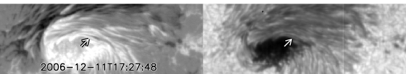
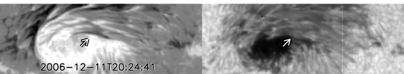
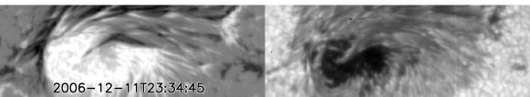
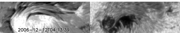
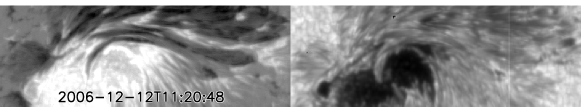
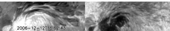
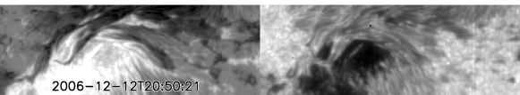
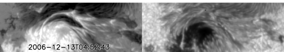
Figure 3: FG $V$/$I$ maps (left) and the corresponding FG $I$ maps (right). Images in the same row are taken at the same time and show the same FOV slightly larger than that of the white box in Figure 1. Arrows in images in the first and the second row are pointing the location of the negative flux thread of our interest that is composing the magnetic channel.

That the appearance of a flux thread is due to its emergence can be verified by checking the temporal and spatial variations of Doppler velocity around the channel structure. Figure 4 shows that before the appearance of the negative flux thread, at 17 UT on December 11, most of the area shows downflows slower than $+0.3$ km s^-1. It is a well-known property that Dopplergrams at active regions generally show downflows of 0.2–$0.3$ km s^-1 (Bhatnagar, 1971; Howard, 1971, 9172; Giovanelli & Slaughter, 1978). About three hours later at 20UT when the thread forms, upflows show up at the center of the PIL, just between the positive spot and the negative thread. This upflow signature is clearer in the spatial profiles of the LOS velocity across the threads presented in the lower panel of Figure 4. At 20 UT on December 11, upflows of about $-0.3$ km s^-1 are seen at the interface between the positive spot and the negative flux thread. As the time goes on, the signature of upflows becomes enhanced with the width of the upflow region along the north–south direction increasing from 0″.7 (20 UT on December 11) to 3″.5 (11UT on December 12), and with the upflow speed increasing from about $-0.3$ to over $-1$ km s^-1 in $19$ hr.

Interestingly, the spatial distribution of the LOS velocity around the negative flux thread at a specific instant, say, at 20 UT on December 11 is consistent with what is expected when an arch-shaped magnetic flux emerges. We expect that the center of a PIL will display blueshifts because of the emerging apex and both footpoints on the opposite sides of the PIL will do redshifts because of the draining plasma along the field line. In fact we see faster downflows of $+1.5$ km s^-1 at both ends of the negative flux thread and slower upflows of $-0.3$ km s^-1 at the center of the PIL.

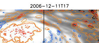
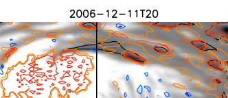
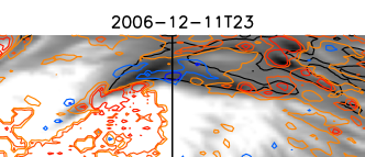
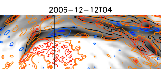
Figure 4: Upper panel (gray-scaled images) : gray-scaled LOS magnetograms aligned with contours of the LOS velocity. The blue/orange contours represent upflow/downflow with the contour levels of $(-1.0,-0.5,-0.2,\,0.5,1.0,1.5)$ km s^-1. Black contours indicate the PILs. The FOV of each image is $43\arcsec\times 16\arcsec$, the same as that of the solid rectangle in Figure 1. The vertical line in each image indicates the position along which the spatial profile of the LOS velocity will be measured. Lower panel (plots) : spatial profiles of the LOS velocity and the LOS magnetic field along the line indicated in each upper panel. Dotted lines indicate the polarity reversals.

With the result of the ME inversion of SP data, we have checked the transverse vector magnetic field and inclination angles around the magnetic channel to figure out the magnetic field configuration of the negative flux thread. Vector magnetograms presented in Figure 5 clearly show that the magnetic field around the channel structure is predominantly horizontal and nearly parallel to the channel. Horizontal fields are as strong as 3000 G while vertical fields are weaker than 1000 G. The shear angles and inclinations of this channel area at a specific time were previously studied by Wang et al. (2008). Here we focus on the beginning phase of the flux emergence and thereafter. The transverse magnetic field vectors at 17 UT on December 11 diverge out of the positive spot, and tightly wind around the umbra clockwise, indicating that this active region is already highly non-potential. Before the channel formation the azimuth of the vectors is smooth and nearly uniform, but as the negative flux thread emerges and grows, it steeply varies across the thread. Combined with the change of magnetic polarity, this spatial variation of azimuth is consistent with a magnetic configuration of negative (left-handed) twist. Considering that the transverse field is already nearly parallel to the channel at the early phase of the flux emergence and that persistent upflows exist along the thread, we think that the twist is continuously carried by the emerging flux from below the surface rather than being induced by the photospheric flows after emergence.

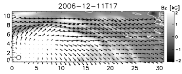
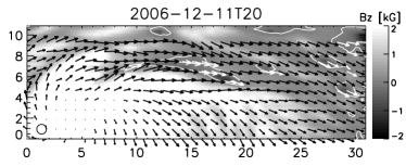
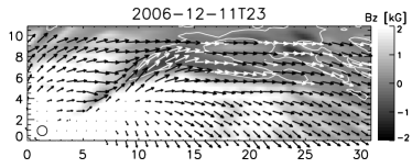
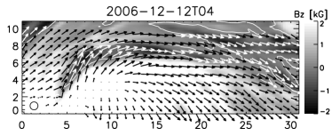
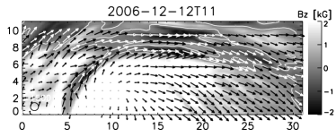
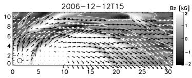
Figure 5: Transverse magnetic field vectors superposed on gray-scaled LOS magnetograms. The unit length of the arrow (the diameter of the circle at the lower left corner) corresponds to the transverse field strength of $2000$ G. The color of arrows was set to be opposite to that of the background gray-scaled magnetogram.

Figure 6 shows that the direction of magnetic field changes from horizontal to vertical at the channel between the positive spot and the negative thread, as the negative flux thread grows. At 17 UT on December 11, before the formation of the magnetic channel most of the region shows nearly $90^{\circ}$ inclination indicating that the magnetic field is almost parallel to the surface. After the thread emerges, the inclination gradually increases and at some places it reaches about $120^{\circ}$ already at 04 UT on December 12. This trend of increase is clearly shown in the time profile of inclination spatially averaged along the negative flux thread. Roughly speaking, the averaged inclination increases from $95^{\circ}$ to $112^{\circ}$ for 22 hr, which means that the magnetic field gradually changes to vertical to the surface. The inclination angle of $112^{\circ}$ means that the field is negative and $22^{\circ}$ inclined from the surface. Together with results on the Doppler velocity described above, this result supports the emergence of arch-shaped magnetic fields.

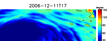
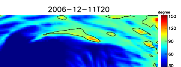
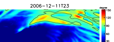
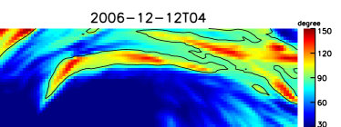
Figure 6: Upper panel : spatial distribution of the inclination angle. An angle of $90^{\circ}$ corresponds to horizontal fields to the surface. Angles either less than $30^{\circ}$ or over $150^{\circ}$ were suppressed in the map in order to describe the change in inclination around the channel more clearly. The inclination angles of the channel are all within $30^{\circ}--150^{\circ}$ range. The black solid contours indicate the PIL. Lower panel : time variation of the inclination angle that was measured and averaged along each negative flux thread.

Figure 7 shows that the vertical component of electric current density is strong along the PIL between the negative flux thread and the positive penumbral magnetic field. The negative flux thread is identified by the enclosing white contour in each panel. The most prominent is the appearance and growth of a pair of current threads of opposite polarity: a negative one in the magnetic region of positive polarity and a positive one in the region of the negative flux thread. Its signature is seen as early as 17 UT on December 11, even before the emergence of the negative flux thread. This pair of current threads is another manifestation of the steep gradient of the transverse component of magnetic field across the flux thread, and is quite consistent with the emergence of a horizontal flux tube that is twisted in the left-handed sense. A careful examination of Figure 7 reveals that after the appearance of the negative flux thread, the current thread of negative polarity gets stronger than the one of positive polarity. This asymmetry may be explained by the interaction of the newly emerging field and pre-existing overlying field. Since the current thread of negative polarity shows up in the region of stronger field, the magnetic flux should be more squeezed, resulting in a steeper magnetic gradient and a higher electric current density.

An opposite pattern of current density is also found in Figure 7: a negative current in the magnetic region of negative polarity, and a positive one in the negative magnetic region. It could be interpreted in two ways. The weaker current threads with the opposite direction to one along the magnetic channel may represent the return current of the twisted flux tube. In the case of the typical twisted flux tube, the surface current flows opposite to the field-aligned volume current so that the twisted flux tube could have a finite size. They are concentrated in the vicinity of the flux thread at the early phase of the flux emergence. The other possible interpretation is that those opposite current threads may indicate that local flux is twisted in the right-handed sense, which is opposite to the twist of magnetic channel structure. It is not surprising if some local magnetic fields emerge carrying opposite helicity to the total helicity of the active region (Kusano et al., 2004; Chandra et al., 2010). However, the current threads are fragmented and get complex as the magnetic channel evolves and more fine-scale flux threads emerge nearby. Therefore, it is not easy to interpret current distribution at the later phase of the channel formation.

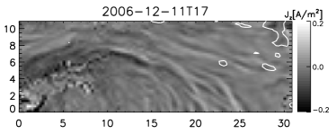
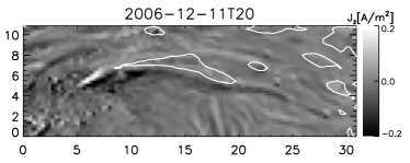
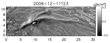
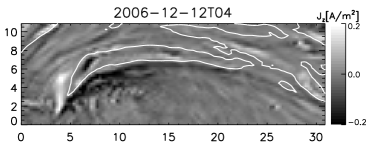
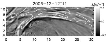
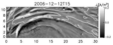
Figure 7: Maps of the vertical components of electric current (gray scale) with the PILs (white contour). The positive sign corresponds to the upward direction and the negative to the downward. The current field stronger than $\pm 0.2$ A m^-2 was suppressed in the image display.

3.2 Coronal Magnetic Field

With the aid of the NLFFF extrapolation, we have checked the temporal change of the coronal magnetic field and the three-dimensional current field above the magnetic channel, assuming that the evolution of the magnetic field in the corona may be approximated to be quasi-static and force-free. Figure 8 displays the field lines that are lower than 3 Mm and near the negative flux thread at each instant. The figure clearly demonstrates the emergence of highly sheared field lines (red lines and blue lines) along the photospheric negative flux thread inside a pre-existing less sheared arcade (yellow lines). Before the appearance of the negative flux thread, at 17 UT on December 11, most of the field lines are over 3 Mm (omitted from the figure) and the lower field lines are connecting the positive and the negative spots. After the negative flux thread emerged, at 23UT, new field lines lower than 1 Mm connecting the positive magnetic region and the negative flux thread (red lines) are observed below yellow lines at 23 UT on December 11. At 04 UT on December 12, the flux thread has grown laterally and blue lines slightly higher than red lines are visible along the flux thread. Since we did not trace the field line footpoints along the time, we could not tell which field line corresponds to which among different observation times. However, since the negative flux thread is continuously emerging, it seems natural to assume that some of the red lines at 23 UT on December 11 extended upward and are seen as blue lines at 04 UT on December 12. The overall topology of field lines at 04 UT on December 12, more sheared field lines inside less sheared ones, resembles the upper portion of a twisted flux tube that has partly emerged through the photosphere. These results from NLFFF extrapolations are consistent with the picture of the emergence of a twisted flux tube. Although Schrijver et al. (2008) and Magara & Tsuneta (2008) also showed evidence of the emerging twisted flux tube in AR 10930, we are looking at somewhat different region in that the scale size of the channel structure is a lot smaller than theirs.

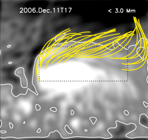
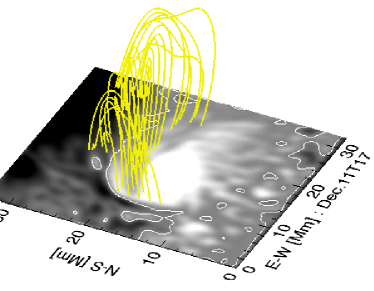
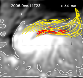
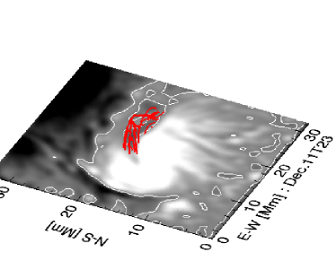
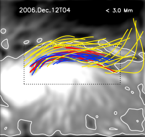
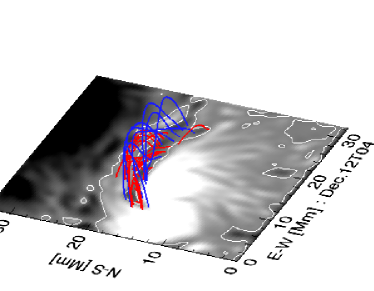
Figure 8: Magnetic field lines from the NLFFF extrapolation viewed from the top (left panel) and side (right panel). Field lines lower than 3 Mm only are displayed co-aligned with the vertical magnetic field (gray scale images). Field lines of the channel structure are colored either red or blue depending on their height, and overlying field lines are colored yellow. Red indicates field lines lower than 1 Mm, blue higher than 1 Mm and lower than 2 Mm. Overlying field lines are omitted in side view images to show the channel field lines clearly.

The NLFFF extrapolations allow us to calculate all the components of electric current density in the lower corona. Figure 9 shows the isosurfaces of the transverse component of current density with the value of $0.1$ A m^-2 taken at 20 UT on December 11 and 4 UT on December 12. The isosurfaces viewed from the top have helical structures that are consistent with the shape of the channel field lines shown in Figure 8. The height of the isosurface at 20 UT on December 12 is about 2 Mm. In fact, as the negative flux thread emerges, the increase of the isosurface is more enhanced in the lateral direction along the PIL than in the vertical direction. The overlying field lines may prohibit the emerging flux from rapidly expanding to the upper layer.

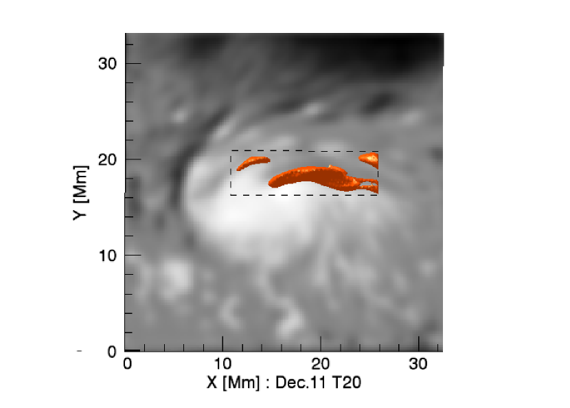
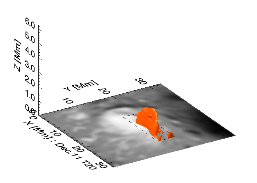
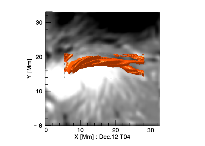
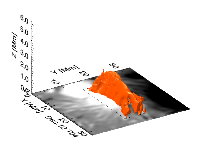
Figure 9: Isosurfaces of the transverse component of current density, $|J_{t}|=\sqrt{{J_{x}}^{2}+{J_{y}}^{2}}=0.1~{}\textrm{A}~{}\textrm{m}^{-2}$, viewed from the top (left) and side (right). The upper panel was taken at 20 UT on December 11 and the lower panel at 04 UT on December 12. Current density out of the rectangle presented by the dashed line was suppressed in the display to show the current density along the channel only.

The left panel of Figure 10 shows the spatial variations of the total current density over the altitude at different observation times. It is clear from the figure that high density of current is confined to heights below about 2 Mm in all observations and the total current density decreases to nearly zero in the higher layer. This trend of decrease in the higher layer is not surprising considering the general expectation that the coronal field gets more potential-like as well as the field strength gets weaker as the altitude increases (Jing et al., 2008). What is more interesting to us is the finding of the narrow vertical extent of the high-density current layer since it implies that the newly emerging flux that carries electric current is vertically confined.

The high-density current layer, even though vertically confined, underwent temporal changes. The right upper panel of Figure 10 presents the time profile of the total current density measured at a fixed height of $0.46$ Mm and shows that the current at this lower layer increases as the channel evolves. This result indicates that the emerging flux thread carries electric current into the lower corona. Moreover, the right lower panel shows that the height of the same total current of $0.16$ A m^-2 increases by about $1.1$ Mm in $27$ hours. This means that the electric current not only increases at the lower layer but also transfers to the upper layer because of the emergence of the flux thread.

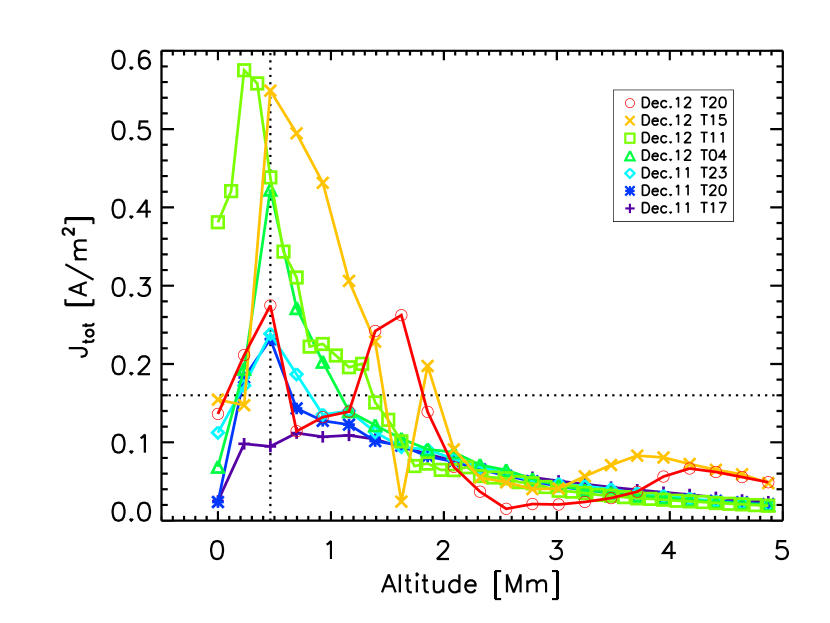
Figure 10: Left panel : total current density $|J_{\textrm{tot}}|=\sqrt{{J_{x}}^{2}+{J_{y}}^{2}+{J_{z}}^{2}}$ over the altitude above the region of the negative flux emergence. Each value of the total current was taken from the average over $3\times 3$ pixels centered on the position of peak height-integrated current density at each altitude. Right panel : Time profiles of the total current density measured at $0.46$ Mm (upper panel) and height at which the value of the total current density is $0.16$ A m^-2 (lower panel).

4 Summary and Discussion

4.1 Formation of the magnetic channel

We have analyzed the formation process of the magnetic channel in AR 10930 in detail, focusing on the region of a negative flux thread that comprises the magnetic channel, and obtained the following results.

1. Negative flux threads that comprise the magnetic channel have elongated shape from the early phase of their emergence, and correspond to penumbral filaments seen in the intensity maps.

2. Upflows of $-0.5$ to $-1.0$ km s^-1 are detected inside the thread and downflows of 1.5–$2.0$ km s^-1 near both tips of the thread.

3. The magnetic fields of the channel structure are highly sheared from the early phase of the formation and their averaged inclination angle increases from $95^{\circ}$ ($5^{\circ}$ inclined from the surface) to $112^{\circ}$ ($22^{\circ}$ inclined from the surface) as the thread emerges.

4. The map of the vertical component of electric current density displays a pair of strong vertical current threads of opposite polarity along the neutral line between the negative flux thread and the positive umbra.

5. The coronal magnetic field computed using the NLFFF extrapolation indicates the emergence of highly sheared arch-shaped field lines inside the slightly sheared arcades that resemble the upper part of the twisted flux tube.

6. The total current density in the lower corona (at the height of $0.46$ Mm) increases (by $0.45$ A m^-2 for 22 hr) and slowly transfers to the upper layer ($\Delta$height$=1.1$ Mm for 27 hr) due to the emergence of the flux thread.

These results indicate that the highly sheared magnetic channel is formed by the subsequent emergence of the current-carrying magnetic fields, rather than the photospheric flow after the flux emergence. In case the emerging field was initially potential and was sheared by the photospheric flow, there should be observed a sufficient amount of velocity gradient of horizontal flows across the neutral line. Horizontal flows parallel to the neutral line but toward opposite directions on each side of the neutral line may stretch and shear the magnetic field. And the amount of the shear, the shear angle, would depend on the velocity gradient across the neutral line. We measured the mean value of the shear angles within a distance of 500 km from the channel’s neutral line and the value was about $72^{\circ}$ at 20 UT on December 12. If we assume that the semi-circular field emerged at a constant emerging speed of $0.5$ – $1.0$ km s^-1, based on the upflow speed obtained from the Dopplergram, then the magnetic field should have been tilted at $72^{\circ}$ within $8$ – $16$ minutes. In this case, the required velocity difference between horizontal flows on each side of the neutral line would be quite large, i.e., $3$ – $6$ km s^-1. However, we could not find such a large velocity difference across the neutral line of the magnetic channel from the time series of FG $V/I$ images. Horizontal flows on each side of the neutral line were toward the same direction and the speed was comparable with the value of around $1$ km s^-1. Therefore, we suggest that the effect of the photospheric flow after the flux emergence may be insignificant in the formation of the magnetic channel.

As a matter of fact, the picture of the formation of the magnetic channel by the emerging magnetic flux was already pointed out by previous studies (Zirin & Wang, 1993; Kubo et al., 2007; Wang et al., 2008). In these studies, the pattern such as negative polarities alternate with positive ones is schematically explained by the emergence of multiple bipoles. Although they conjectured that these emerging bipoles are likely to be carrying shear and twist into the corona, however, their studies were insufficient to reveal where and how the shear or twist was supplied. In contrast, our study investigates the very early phase of the flux emergence and provides strong evidence that each emerging flux that comprises the magnetic channel is actually a fine-scale twisted flux tube.

Our study indicates that the elongated shape of the negative magnetic flux thread constituting the magnetic channel is an intrinsic property of its own rather than a result of either stretching by horizontal motions (Zirin & Wang, 1993) or squeezing by surrounding magnetic flux (Wang et al., 2008). The flux thread corresponds to a penumbral filament seen in the intensity maps, and these two features appear to be two different manifestations of the same structure: an emerging twisted flux tube. This result is in line with the study of Bellot Rubio et al. (2007) who found the evidence that supports the idea that the dark-cored penumbral filaments may be flux tubes carrying Evershed flows.

4.2 NLFFF extrapolation in the lower corona

The narrow width of the magnetic channel observed in the photospheric magnetograms hints that its vertical extension may be also quite low, comparable to the size of its width. Both reconstructed magnetic fields (Figure 8) and the isosurface of transverse current density (Figure 9) also indicate that the channel structure lies in the lower atmosphere corresponding to chromospheric level. Then it should be checked if it is reasonable to apply the NLFFF extrapolation to such a low atmosphere. We have compared the extrapolated field lines lower than 2 Mm and chromospheric structures observed in a Ca II image taken by SOT/Hinode (Figure 11). The field lines in the left panel of Figure 11 relatively well follow the topology of chromospheric structures in the Ca II image. Note that the region where we reconstructed NLFFF is the center of the strong active region. The unsigned field strength at the photosphere is over 3000 G in the positive polarity and over 2000 G in most of the interested region. Therefore, we expect that the plasma-$\beta$ would be less than unity in the upper chromosphere of the active region and the force-free assumption could be reliably applied in such a low portion. The plasma-$\beta$ model derived by Gary (2001) also shows that $\beta<1$ at around 2 Mm above an active region although its value depends on both the magnetic and the pressure model they chose.

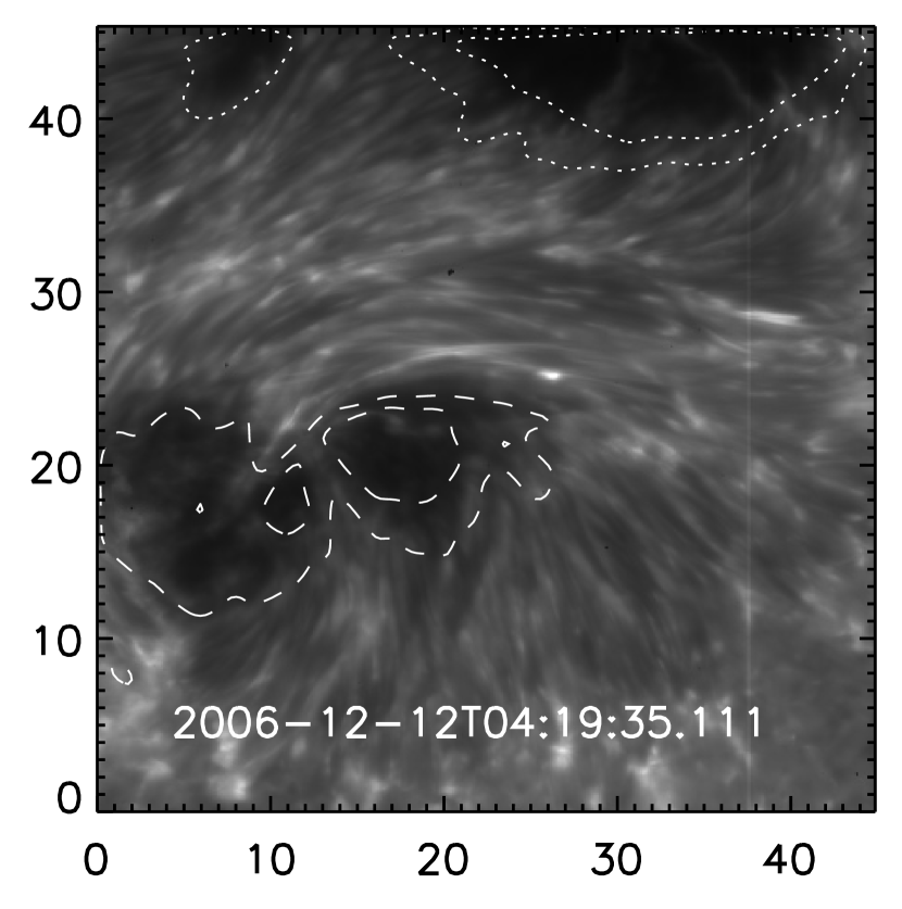
Figure 11: Left panel : magnetic field lines reconstructed from the NLFFF extrapolation of which height is less than 2 Mm. Right panel : Ca II image with the same FOV as the bottom boundary condition of the NLFFF extrapolation. Dotted lines indicate isocontours of negative polarity and dashed lines positive polarity of the bottom vertical magnetogram in both panels.

4.3 Relationship with flares

Is the formation of the magnetic channel important in the occurrence of flares? Our finding that strong current flows along the flux thread that comprises the magnetic channel suggests a positive answer to this question. It has been frequently pointed out that the flux emergence already carrying currents and helicity in the active region helps to add magnetic free energy into the region (Ishii et al., 1998; Brooks et al., 2003). Adding magnetic free energy could destabilize the pre-existing magnetic field in active region so that it may be subject to more eruptive events such as flares, coronal mass ejections and filament eruptions. Recently, increasing evidence is suggested from observations that support the idea of emerging currents associated with the emerging twisted magnetic flux from below the photosphere (Kurokawa, 1987; Tanaka, 1991; Leka et al., 1996; Ishii et al., 1998; Schrijver et al., 2008).

Our another finding that the electric current is confined to below 2 Mm above the surface, however, seems to make a problem. This height is too low for the expected height of the reconnection that produces the flare. Based on the standard flare model and considering the size and distance of the two-ribbon footpoints, the reconnection in charge of major flares should occur at the height of around 10 Mm, which is much higher than 2 Mm. One probable solution to this problem is to suppose that the strong electric current is gradually transferred to the higher layer, as is implied from our results from NLFFF models and would form the current sheet there, an essential component of the reconnection. Moreover, magnetic reconnection is likely to occur between newly emerging flux and pre-existing ambient field and can also play a role in transferring the free magnetic energy carried by the emerging flux tube to the overlying coronal field. Since the emergence of the flux thread, brightening was continuously detected along the flux thread in the Ca II images taken by SOT/Hinode. This brightening may represent subsequent magnetic reconnection of this kind, through which we may relate the emerging flux tube of much smaller scale to the December 13 flare with much larger size. Summing up, it seems that the formation of magnetic channel in AR 10930 plays a role in the December 13 flare in that it destabilizes the ambient magnetic field by carrying free energy into the corona.

4.4 Fine structure of AR magnetic fields

This study on the flux thread gives us implications not only on the structure of magnetic channel itself but also on the fine structure of an active region magnetic field. In the case of AR 10930, Schrijver et al. (2008) and Magara & Tsuneta (2008) already suggested the emergence of a twisted flux tube by retrieving coronal magnetic fields using the NLFFF extrapolation and by checking the temporal variation of the shear angle along the PIL, respectively. Compared to the scale size of their interests, the channel structure we focused on is a lot smaller, a few Mm in height. Then how could it be explained that twisted flux tubes in different scale size coexist in the same region? It seems that the magnetic fields of channel structure may be a sub-structure of larger scaled flux tube. The simple model of an active region commonly adopted is that the whole active region is a twisted flux tube. This assumption frequently well describes the large-scale structure of an active region such as sigmoid in coronal observations. However, as we observe active regions with higher spatial resolution, we find more complex and fragmentary magnetic structures, such as magnetic channel in our case. It gives us an impression that the active region as a whole twisted flux tube consists of a number of segments of twisted flux ropes. The successive emergence of small-scale flux often has been explained by the emergence of undulating single or multiple flux ropes (Ishii et al., 1998; Low, 2001; Kurokawa et al., 2002; Schrijver, 2009). The formation of active region filaments is also explained by emergence of twisted flux tube by some authors (Lites et al., 1995; Okamoto et al., 2008). Depending on the size of these segments of twisted flux rope, different features would be observed at the photosphere.

References

- Bellot Rubio et al. (2007) Bellot Rubio, L. R., et al. 2007, ApJ, 668, L91
- Bhatnagar (1971) Bhatnagar, A. 1971, Sol. Phys., 16, 40B
- Brooks et al. (2003) Brooks, D. H., Kurokawa, H., Yoshimura, K., Kozu, H., & Berger, T. E. 2003, A&A, 411, 273
- Chae et al. (2007) Chae, J., et al. 2007, PASJ, 59, 619
- Chandra et al. (2010) Chandra, R., Pariat, E., Schmieder, B., Mandrini, C., H., & Uddin, W., 2010, Sol. Phys., 261, 127
- Gary (2001) Gary, G. A. 2001, Sol. Phys., 203, 71
- Giovanelli & Slaughter (1978) Giovanelli, R. G., & Slaughter, C. 1978, Sol. Phys., 57, 255G
- Guo & Ding (2008) Guo, Y., & Ding, M. D. 2008, ApJ, 679, 1629
- Hagyard et al. (1984) Hagyard, M. J., Smith, J. B., Jr., Teuber, D., & West, E. A. 1984, Sol. Phys., 91, 115
- Hagyard et al. (1990) Hagyard, M. J., Venkatakrishnan, P., & Smith, J. B., Jr. 1990, ApJS, 73, 159
- Howard (1971) Howard, R. 1971, Sol. Phys., 16, 21H
- Howard (9172) Howard, R. 1972, Sol. Phys., 24, 123
- Ishii et al. (1998) Ishii, T. T., Kurokawa, H., & Takeuchi, T. T. 1998, ApJ, 499, 898
- Jing et al. (2008) Jing, J., Wiegelmann, T., Suematsu, Y., Kubo, M., & Wang, H. 2008, ApJ, 676, L81
- Jing et al. (2009) Jing, J., Tan, C., Yuan, Y., Wang, B., Wiegelmann, T., Xu, Y., & Wang, H. 2010, ApJ, 713, 440
- Kubo et al. (2007) Kubo, M., et al. 2007, PASJ, 59, 779
- Kurokawa (1987) Kurokawa, H. 1987, Sol. Phys., 113, 259
- Kurokawa et al. (2002) Kurokawa, H., Wang, T., & Ishii, T. T. 2002, ApJ, 572, 598
- Kusano et al. (2004) Kusano, K., Maeshiro, T., Yokoyama, T., & Sakurai, T. 2004, ApJ, 610, 537
- Leka et al. (1996) Leka, K. D., Canfield, R. C., McClymont, A. N., & van Driel-Gesztelyi, L. 1996, ApJ, 462, 547
- Lites et al. (1995) Lites, B. W., Low, B. C., Martínez Pillet, V., Seagraves, P., Skumanich, A., Frank, Z., Shine, R. A., & Tsuneta, S. 1995, ApJ, 446, 877
- Low (2001) Low, B. C. 2001, J. Geophys. Res., 106, 25141
- Magara & Tsuneta (2008) Magara, T., & Tsuneta, S. 2008, PASJ, 60, 1181
- Min & Chae (2009) Min, S., & Chae, J. 2009, Sol. Phys., 258, 203
- Moon et al. (2003) Moon, Y. -J., Wang, H., Spirock, T. J., Goode, P. R., & Park, Y. D. 2003, Sol. Phys., 217, 79
- Moon et al. (2007) Moon, Y. -J. et al. 2007, PASJ, 59, 625
- Okamoto et al. (2008) Okamoto, T. J., et al. 2008, ApJ, 673, L215
- Rees & Semel (1979) Rees, D. E., & Semel, M. D. 1979, A&A, 74, 1
- Schrijver et al. (2008) Schrijver, C. J. et al. 2008, ApJ, 675, 1637
- Schrijver (2009) Schrijver, C. J. 2009, Adv. Space Res., 43, 739
- Tanaka (1991) Tanaka, K. 1991, Sol. Phys., 136, 133
- Uitenbroek (2003) Uitenbroek, H. 2003, ApJ, 592, 1225
- Wang et al. (1996) Wang, J., Shi, Z., Wang, H., & Lü, Y. 1996, ApJ, 456, 861
- Wang (2006) Wang, H. 2006, ApJ, 649, 490
- Wang et al. (2008) Wang, H., Jing, J., Tan, C., Wiegelmann, T., & Kubo, M. 2008, ApJ, 687, 658
- Wiegelmann (2004) Wiegelmann, T. 2004, Sol. Phys., 219, 87
- Wiegelmann & Inhester (2006) Wiegelmann, T., & Inhester, B. 2006, Sol. Phys., 233, 215
- Zirin & Wang (1993) Zirin, H., & Wang, H. 1993, Nature, 363, 426