Direct regular-to-chaotic tunneling rates using the fictitious integrable system approach

Abstract

We review the fictitious integrable system approach which predicts dynamical tunneling rates from regular states to the chaotic region in systems with a mixed phase space. It is based on the introduction of a fictitious integrable system that resembles the regular dynamics within the regular island. We focus on the direct regular-to-chaotic tunneling process which dominates, if nonlinear resonances within the regular island are not relevant. For quantum maps, billiard systems, and optical microcavities we find excellent agreement with numerical rates for all regular states.

I Introduction

Tunneling of a particle is one of the central manifestations of quantum mechanics. The prototypical example is the tunneling escape from a one-dimensional potential well through an energy barrier. While classically the particle is confined for all times, quantum mechanically the probability inside the well decays exponentially, $\exp(-\gamma t)$, where $\gamma$ is the tunneling rate. It depends on the width and the height of the barrier and can be predicted, e.g., using WKB theory LanLif1991 . Tunneling vanishes in the semiclassical limit, where typical classical actions are large compared to Planck’s constant.

Tunneling not only occurs for potential barriers but whenever the corresponding classical system consists of dynamically disconnected regions in phase space, which has been termed dynamical tunneling DavHel1981 . It occurs in Hamiltonian systems which typically have a mixed phase space. Here regions of regular motion, the so-called regular islands, and regions of chaotic motion, the so-called chaotic sea, coexist. While the classical motion is confined to any of these regions, quantum mechanically they are coupled by dynamical tunneling. In particular the fundamental process of regular-to-chaotic tunneling describes the exponential decay of a wave packet initially localized in the regular island to the chaotic sea. The same coupling also leads to tunneling from the chaotic sea to the regular island.

Dynamical tunneling also affects the structure of eigenstates of systems with a mixed phase space. According to the semiclassical eigenfunction hypothesis Per1973 ; Ber1977 ; Vor1979 the eigenstates are concentrated either in the regular islands or in the chaotic sea. Away from the semiclassical limit this classification still holds approximately such that the corresponding eigenstates are called regular or chaotic. However, each eigenstate has contributions in the other regions of phase space, due to dynamical tunneling.

Dynamical tunneling in a mixed phase space has been studied theoretically HanOttAnt1984 ; Wil1986 ; BohTomUll1993 ; TomUll1994 ; Tom1998 ; Cre1998 ; ShuIke1995 ; ShuIke1998 ; OniShuIkeTak2001 ; BohBooEgyMar1993 ; DorFri1995 ; FriDor1998 ; BroSchUll2001 ; BroSchUll2002 ; EltSch2005 ; SchEltUll2005 ; WimSchEltBuc2006 ; MouEltSch2006 ; Mou2007 ; DenMou2010 ; Kes2005 ; Kes2005b ; PodNar2003 ; PodNar2005 ; SheFisGuaReb2006 ; BarBet2007 ; BaeKetLoeSch2008 ; BaeKetLoeRobVidHoeKuhSto2008 ; BaeKetLoeWieHen2009 ; LoeBaeKetSch2010 ; KesSch2011b and experimentally, e.g., in cold atom systems SteOskRai2001 ; HenHafBroHecHelMcKMilPhiRolRubUpc2001 ; MouDel2003 , microwave billiards DemGraHeiHofRehRic2000 ; HofAltDemGraHarHeiRehRic2005 ; BaeKetLoeRobVidHoeKuhSto2008 , and semiconductor nanostructures FroWilHayEavSheMIuHen2002 . It is of current interest for, e.g., eigenstates affected by flooding of regular islands SchOttKetDit2001 ; BaeKetMon2005 ; BaeKetMon2007 ; Bit2010 , emission properties of optical microcavities WieHen2006 ; BaeKetLoeWieHen2009 ; ShiHarFukHenSasNar2010 ; YanLeeMooLeeKimDaoLeeAn2010 , and spectral statistics in systems with a mixed phase space PodNar2007 ; VidStoRobKuhHoeGro2007 ; BatRob2010 ; BaeKetLoeMer2010 .

The concept of chaos-assisted tunneling was introduced in Refs. BohTomUll1993 ; TomUll1994 ; Tom1998 . It occurs, e.g., in systems with two symmetry-related regular islands surrounded by chaotic motion in phase space. There it was observed that the energy splittings $\Delta E$ between two symmetry related regular states are typically drastically enhanced due to the appearance of chaotic states, compared to an integrable situation. Chaos-assisted tunneling consists of two processes: a regular-to-chaotic tunneling step from a regular torus of one island to the chaotic sea and a chaotic-to-regular tunneling step from the chaotic sea to the symmetry-related torus. The energy splittings $\Delta E$ show strong fluctuations LinBal1990 ; BohTomUll1993 ; TomUll1994 ; Tom1998 under variation of external parameters, as the distance between the energies of the regular doublet and the close-by chaotic states varies. This was also observed for optical microcavities PodNar2005 and microwave billiards DemGraHeiHofRehRic2000 ; HofAltDemGraHarHeiRehRic2005 . In contrast to the energy splittings $\Delta E$ the regular-to-chaotic tunneling rates $\gamma$ describe the average coupling to the chaotic sea, $\gamma=\langle\Delta E\rangle/\hbar$, as shown in Sec. II.4, and therefore do not fluctuate.

In the regime, $h\lesssim A_{\text{reg}}$, in which the Planck constant $h$ is smaller but of the same order as the area $A_{\text{reg}}$ of the regular island, quantum mechanics is not affected by fine-scale structures in phase space, such as nonlinear resonances or the hierarchical transition region. Hence, the direct regular-to-chaotic tunneling process dominates. In Ref. HanOttAnt1984 a qualitative argument for the tunneling rates to behave exponentially as $\gamma\propto\exp(-B/h)$ was given. One may write $B=CA_{\text{reg}}$, where the non-universal constant $C$ has been calculated for various situations in the semiclassical limit: For a weakly chaotic system $C=2\pi$ SheFisGuaReb2006 was found and $C>2\pi$ for rough nanowires FeiBaeKetRotHucBur2006 ; FeiBaeKetBurRot2009 . The approach in Ref. PodNar2003 leads semiclassically to $C=2-\ln 4$ which was corrected to $C=3-\ln 4$ She2005 . However, this prediction does not describe generically shaped regular islands as it uses a transformation of the regular island to a harmonic oscillator.

In order to find a quantitative prediction of direct regular-to-chaotic tunneling rates for generic islands we introduced the fictitious integrable system approach BaeKetLoeSch2008 ; Loe2010 . It relies on the decomposition of Hilbert space into a regular and a chaotic subspace by means of a fictitious integrable system BohTomUll1993 ; PodNar2003 ; SheFisGuaReb2006 . We require that its dynamics resembles the regular motion in the originally mixed system as closely as possible and extends it beyond the regular region. This leads to a tunneling formula involving properties of this integrable system as well as its difference to the mixed system under consideration. It allows for the prediction of tunneling rates from any quantized torus within the regular island. This approach was applied to quantum maps BaeKetLoeSch2008 , billiard systems BaeKetLoeRobVidHoeKuhSto2008 , and optical microcavities BaeKetLoeWieHen2009 .

In the semiclassical regime, $h\ll A_{\text{reg}}$, the fine-scale structures of the classical phase space can be resolved by quantum mechanics. In particular, nonlinear resonances cause an enhancement of the regular-to-chaotic tunneling rates, which has been termed resonance-assisted tunneling BroSchUll2001 ; BroSchUll2002 ; EltSch2005 ; SchEltUll2005 . It leads to characteristic peak and plateau structures in the tunneling rates as observed for near integrable systems BroSchUll2001 ; BroSchUll2002 , mixed quantum maps EltSch2005 ; SchEltUll2005 , periodically driven systems MouEltSch2006 ; WimSchEltBuc2006 , quantum accelerator modes SheFisGuaReb2006 , and for multidimensional molecular systems Kes2005 ; Kes2005b . Quantitatively, however, deviations of several orders of magnitude to numerical rates appear, especially in the experimentally accessible regime where nonlinear resonances become relevant for tunneling. Recently, it was shown that a combination of the direct regular-to-chaotic tunneling mechanism and the resonance-assisted tunneling mechanism leads to a theory which quantitatively predicts tunneling rates from the quantum to the semiclassical regime LoeBaeKetSch2010 . For the application of this unified theory it is essential to determine the direct regular-to-chaotic tunneling rates.

In this paper we review the fictitious integrable system approach for the prediction of direct regular-to-chaotic tunneling rates. The approach is derived in Sec. II. Numerical methods for the determination of tunneling rates are presented in Sec. III. It is then shown how the approach can be applied analytically, semiclassically, and numerically to quantum maps in Sec. IV and two-dimensional billiard systems in Sec. V.

II Dynamical tunneling and the fictitious integrable system approach

We consider systems with a mixed phase space, in particular two-dimensional quantum maps and billiards. Their phase space is divided into regions of regular dynamics and regions of chaotic dynamics. We focus on the fundamental situation of just one regular island embedded in the chaotic sea, Fig. 1(a). At the center of the island one has an elliptic fixed point, which is surrounded by invariant regular tori. For such systems the semiclassical eigenfunction hypothesis Per1973 ; Ber1977 ; Vor1979 implies that in the semiclassical limit the eigenstates can be classified as either regular or chaotic, according to the phase-space region on which they concentrate. In order to understand the behavior of eigenstates away from the semiclassical limit one has to compare the size of phase-space structures with Planck’s constant $h$. We discuss this exemplarily for quantum maps BerBalTabVor1979 which are described by a unitary time-evolution operator $U$ on a Hilbert space of finite dimension $N$. Here we introduce the semiclassical parameter $h_{\text{eff}}=h/A=1/N$ as the ratio of Planck’s constant $h$ to the area $A$ of phase space. The eigenstates $|\psi_{n}\rangle$ and quasi-energies $\varphi_{n}$ of $U$ are determined by

$$U|\psi_{n}\rangle=\text{e}^{\text{i}\varphi_{n}}|\psi_{n}\rangle.$$ (1)

The so-called regular states are predominantly concentrated on tori within the regular island and fulfill the Bohr-Sommerfeld type quantization condition

$$\oint p\,\text{d}q=h_{\text{eff}}\left(m+\frac{1}{2}\right),\quad m=0,\dots,N_{\text{reg}}-1.$$ (2)

For a given value of $h_{\text{eff}}$ there exist $N_{\text{reg}}$ of such regular states, where $N_{\text{reg}}=\lfloor A_{\text{reg}}/h_{\text{eff}}+1/2\rfloor$ and $A_{\text{reg}}$ from now on is the dimensionless area of the regular island. The chaotic states mainly extend over the chaotic sea. Note, that for systems with a large density of chaotic states the regular states may disappear and chaotic states flood the regular island BaeKetMon2005 ; BaeKetMon2007 .

An important consequence of a finite $h_{\text{eff}}$ in systems with a mixed phase space is dynamical tunneling. It couples the regular island and the chaotic sea, which are classically separated. Hence, the regular and chaotic eigenfunctions of $U$ always have a small component in the other region of phase space, respectively, see Fig. 1(b,c).

The coupling of the regular and the chaotic phase-space regions can be quantified by tunneling rates $\gamma_{m}$ which describe the decay from the $m$th regular torus to the chaotic sea. To define these tunneling rates one can consider a wave packet started on this $m$th quantized torus in the regular island which is coupled to a continuum of chaotic states, as in the case of an infinite chaotic sea. Its decay $\text{e}^{-\gamma_{m}t}$ is characterized by a tunneling rate $\gamma_{m}$. For systems with a finite phase space this exponential decay occurs at most up to the Heisenberg time $\tau_{H}=h_{\text{eff}}/\Delta_{\text{ch}}$, where $\Delta_{\text{ch}}$ is the mean level spacing of the chaotic states. Alternatively, the tunneling rates can be obtained from lifetimes of resonances in a corresponding open system, e.g., by adding an absorbing region somewhere in the chaotic component, see Sec. III.1.

In the regime, $h_{\text{eff}}\lesssim A_{\text{reg}}$, where $h_{\text{eff}}$ is smaller but comparable to the area $A_{\text{reg}}$ of the regular island, the rates $\gamma_{m}$ are dominated by the direct regular-to-chaotic tunneling mechanism, while contributions from resonance-assisted tunneling are negligible. We concentrate on systems where additional phase-space structures within the chaotic sea are not relevant for tunneling. In the following we derive a prediction for the direct regular-to-chaotic tunneling rates using the fictitious integrable system approach BaeKetLoeSch2008 .

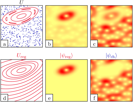
Figure 1: (Color online) (a) Illustration of the mixed classical phase space corresponding to a quantum map $U$ together with the Husimi representation of (b) a regular and (c) a chaotic eigenstate of $U$ which both have a small component in the other region. (d) Illustration of the classical phase space of the fictitious integrable system $U_{\text{reg}}$. (e) Eigenstates $|\psi_{\text{reg}}\rangle$ of $U_{\text{reg}}$ are purely regular, while (f) the purely chaotic states $|\psi_{\text{ch}}\rangle$ extend in the chaotic region of phase space.

II.1 Derivation

In order to find a prediction for the direct regular-to-chaotic tunneling rates we decompose the Hilbert space of the quantum map $U$ into two parts which correspond to the regular and chaotic regions. While classically such a decomposition is unique, quantum mechanically this is not the case due to the uncertainty principle. We find a decomposition by introducing a fictitious integrable system $U_{\text{reg}}$. Related ideas were presented in Refs. BohTomUll1993 ; PodNar2003 ; SheFisGuaReb2006 . The fictitious integrable system has to be chosen such that its dynamics resembles the classical motion corresponding to $U$ within the regular island as closely as possible and continues this regular dynamics beyond the regular island of $U$, see Fig. 1(d). The eigenstates $|\psi_{\text{reg}}^{m}\rangle$ of $U_{\text{reg}}$, $U_{\text{reg}}|\psi_{\text{reg}}^{m}\rangle=\text{e}^{\text{i}\varphi_{\text{reg}}^{m}}|\psi_{\text{reg}}^{m}\rangle$, are purely regular in the sense that they are localized on the $m$th quantized torus of the regular region and continue to decay beyond this regular region, see Fig. 1(e). This is the decisive property of $|\psi_{\text{reg}}^{m}\rangle$ which have no chaotic admixture, in contrast to the predominantly regular eigenstates of $U$, see Fig. 1(b). The explicit construction of $U_{\text{reg}}$ is discussed in Sec. II.2.

With the eigenstates $|\psi_{\text{reg}}^{m}\rangle$ of $U_{\text{reg}}$ we define a projection operator

$$P_{\text{reg}}:=\sum_{m=0}^{N_{\text{reg}}-1}|\psi_{\text{reg}}^{m}\rangle\langle\psi_{\text{reg}}^{m}|,$$ (3)

using the first $N_{\text{reg}}$ eigenstates of $U_{\text{reg}}$ which approximately projects onto the regular island corresponding to $U$. The orthogonal projector

$$P_{\text{ch}}:=\mathds{1}-P_{\text{reg}}$$ (4)

approximately projects onto the chaotic phase-space region. These projectors, $P_{\text{reg}}$ and $P_{\text{ch}}$, define our decomposition of the Hilbert space into a regular and a chaotic subspace.

Introducing a basis $|\psi_{\text{ch}}\rangle$ in the chaotic subspace we can write $P_{\text{ch}}=\sum_{\text{ch}}|\psi_{\text{ch}}\rangle\langle\psi_{\text{ch}}|$. Here we sum over all $N_{\text{ch}}=N-N_{\text{reg}}$ states $|\psi_{\text{ch}}\rangle$, which we call purely chaotic states, see Fig. 1(f) for an illustration. The coupling matrix element $v_{\text{ch},m}$ between a purely regular state $|\psi_{\text{reg}}^{m}\rangle$ and any purely chaotic state $|\psi_{\text{ch}}\rangle$ is

$$v_{\text{ch},m}=\langle\psi_{\text{ch}}|U|\psi_{\text{reg}}^{m}\rangle.$$ (5)

From this the tunneling rate is obtained using a dimensionless version of Fermi’s golden rule, see Appendix A,

$$\gamma_{m}=\sum_{\text{ch}}|v_{\text{ch},m}|^{2},$$ (6)

where the sum is over all chaotic basis states $|\psi_{\text{ch}}\rangle$ and thus averages the modulus squared of the fluctuating matrix elements $v_{\text{ch},m}$. Here we apply Fermi’s golden rule in the case of a discrete spectrum, which is possible if one considers the decay $\text{e}^{-\gamma_{m}t}$ up to the Heisenberg time $\tau_{H}=h_{\text{eff}}/\Delta_{\text{ch}}$ only.

Inserting Eq. (5) into Eq. (6) we obtain

$$\gamma_{m}=\|P_{\text{ch}}U|\psi_{\text{reg}}^{m}\rangle\|^{2}=\|(\mathds{1}-P_{\text{reg}})U|\psi_{\text{reg}}^{m}\rangle\|^{2}$$ (7)

as the basis of all our following investigations. It allows for the prediction of tunneling rates from a regular state localized on the $m$th quantized torus to the chaotic sea. Equation (7) agrees with the intuition that the tunneling rates are determined by the amount of probability that is transferred to the chaotic region after one application of the time evolution operator $U$ on $|\psi_{\text{reg}}^{m}\rangle$. We want to emphasize that Eq. (7) essentially relies on the chosen decomposition of Hilbert space determined by the fictitious integrable system $U_{\text{reg}}$. A similar expression for the tunneling rates was obtained from a phenomenological Hamiltonian in Ref. SheFisGuaReb2006 . Note, that the tunneling rate for the inverse process of tunneling from the chaotic sea to the $m$th regular torus is also given by Eq. (7) but with an additional prefactor of $1/N_{\text{ch}}$ due to the different density of final states Bit2010 .

II.1.1 Approximation for very good $U_{\text{reg}}$

In cases where one finds a fictitious integrable system $U_{\text{reg}}$ which resembles the dynamics within the regular island of $U$ with very high accuracy, Eq. (7) can be approximated as

$$\gamma_{m} \approx \|(U-U_{\text{reg}})|\psi_{\text{reg}}^{m}\rangle\|^{2},$$ (8)

using $P_{\text{reg}}U|\psi_{\text{reg}}^{m}\rangle\approx P_{\text{reg}}U_{\text{reg}}|\psi_{\text{reg}}^{m}\rangle=U_{\text{reg}}|\psi_{\text{reg}}^{m}\rangle$. Instead of the projector $P_{\text{ch}}$ in Eq. (7) the difference $U-U_{\text{reg}}$ enters in Eq. (8). This allows for a semiclassical evaluation, which is presented in Sec. II.3.

II.1.2 Approximation for non-orthogonal chaotic states

If one constructs chaotic states $|\widetilde{\psi}_{\text{ch}}\rangle$ from random wave models Ber1977 , they will not be orthogonal to the purely regular states $|\psi_{\text{reg}}^{m}\rangle$. In this case we construct orthonormalized states

$$|\psi_{\text{ch}}\rangle := c\,(\mathds{1}-P_{\text{reg}})|\widetilde{\psi}_{\text{ch}}\rangle$$ (9)

with normalization $c$. We find for the coupling matrix elements, Eq. (5),

$$v_{\text{ch},m} = c\langle\widetilde{\psi}_{\text{ch}}|U-P_{\text{reg}}U|\psi_{\text{reg}}^{m}\rangle$$ (10)

$$\approx \langle\widetilde{\psi}_{\text{ch}}|U-U_{\text{reg}}|\psi_{\text{reg}}^{m}\rangle,$$ (11)

where we use the approximations $c\approx 1$ and again $P_{\text{reg}}U|\psi_{\text{reg}}^{m}\rangle\approx U_{\text{reg}}|\psi_{\text{reg}}^{m}\rangle$. Equation (11) can now be inserted into Eq. (6), leading to

$$\gamma_{m} \approx \|\widetilde{P}_{\text{ch}}(U-U_{\text{reg}})|\psi_{\text{reg}}^{m}\rangle\|^{2}$$ (12)

with $\widetilde{P}_{\text{ch}}=\sum_{\text{ch}}|\widetilde{\psi}_{\text{ch}}\rangle\langle\widetilde{\psi}_{\text{ch}}|$.

II.1.3 Application to billiards

Two-dimensional billiard systems, which we consider in Sec. V, are given by the motion of a free particle of mass $M$ in a domain $\Omega$ with elastic reflections at its boundary $\partial\Omega$. Quantum mechanically they are described by a Hamilton operator $H$. The fictitious integrable system approach can also be applied to billiards: We use a fictitious integrable system $H_{\text{reg}}$ and its eigenstates $\psi_{\text{reg}}^{mn}(\boldsymbol{q})$, characterized by the two quantum numbers $m$ and $n$. We start from a random wave model Ber1977 for the chaotic states $\widetilde{\psi}_{\text{ch}}(\boldsymbol{q})$ which are not orthogonal to the purely regular states. Using the approximation for non-orthogonal chaotic states we obtain in analogy to Eq. (11)

$$V_{\text{ch},mn}=\int\limits_{\Omega}\text{d}^{2}q\,\widetilde{\psi}_{\text{ch}}(\boldsymbol{q})(H-H_{\text{reg}})\psi_{\text{reg}}^{mn}(\boldsymbol{q})$$ (13)

for the coupling matrix element between a purely regular state with quantum numbers $(m,n)$ and different chaotic states $\widetilde{\psi}_{\text{ch}}(\boldsymbol{q})$. The tunneling rate $\Gamma_{mn}$ is obtained using Fermi’s golden rule, Eq. (121),

$$\Gamma_{mn}=\frac{2\pi}{\hbar}\langle|V_{\text{ch},mn}|^{2}\rangle\,\rho_{\text{ch}}\approx\frac{\mathcal{A}_{\text{ch}}\hbar}{4M}\langle|V_{\text{ch},mn}|^{2}\rangle$$ (14)

where we average over the modulus squared of coupling matrix elements $V_{\text{ch},mn}$ between one particular purely regular state and different chaotic states of similar energy. The chaotic density of states $\rho_{\text{ch}}$ is approximated by the leading Weyl term $\rho_{\text{ch}}\approx\mathcal{A}_{\text{ch}}\hbar^{2}/(8\pi M)$ in which $\mathcal{A}_{\text{ch}}$ denotes the area of the billiard times the chaotic fraction of phase space. This expression for $\rho_{\text{ch}}$ follows, e.g., from counting the number of Planck cells $h^{2}$ in the chaotic part of phase space BohTomUll1993 .

II.2 Fictitious integrable system

The most difficult step in the application of Eqs. (7) and (14) to a given system is the determination of the fictitious integrable system $H_{\text{reg}}$. Its dynamics should resemble the classical motion of the considered mixed system within the regular island as closely as possible. As a result the contour lines of the corresponding integrable Hamiltonian $H_{\text{reg}}$, Fig. 1(d), approximate the KAM-curves of the classically mixed system, Fig. 1(a), in phase space. This resemblance is not possible with arbitrary precision as the integrable approximation for example does not contain nonlinear resonance chains and small embedded chaotic regions. Moreover, it cannot account for the hierarchical regular-to-chaotic transition region at the border of the regular island. Similar problems appear for the analytic continuation of a regular torus into complex space due to the existence of natural boundaries Wil1986 ; Cre1998 ; ShuIke1995 ; ShuIke1998 ; OniShuIkeTak2001 ; BroSchUll2001 ; BroSchUll2002 ; EltSch2005 . However, for not too small $h_{\text{eff}}$, where these small structures are not yet resolved quantum mechanically, an integrable approximation with finite accuracy turns out to be sufficient for a prediction of the tunneling rates.

In addition the integrable dynamics of $H_{\text{reg}}$ should extrapolate smoothly beyond the regular island of $H$. This is essential for the quantum eigenstates of $H_{\text{reg}}$ to have correctly decaying tunneling tails. According to Eq. (7) they are relevant for the determination of the tunneling rates. While typically tunneling from the regular island occurs to regions within the chaotic sea close to the border of the regular island, there exist other cases, where it occurs to regions deeper inside the chaotic sea, as studied in Ref. SheFisGuaReb2006 . Here $H_{\text{reg}}$ has to be constructed such that its eigenstates have the correct tunneling tails up to this region, see Sec. IV.1.3.

For quantum maps we determine the fictitious integrable system in the following way: We employ classical methods, see below, to obtain a one-dimensional time-independent Hamiltonian $H_{\text{reg}}(q,p)$ which is integrable by definition and resembles the classically regular motion of the mixed system. After its quantization we obtain the regular quantum map $U_{\text{reg}}=\text{e}^{-\text{i}H_{\text{reg}}/\hbar_{\text{eff}}}$ with corresponding eigenfunctions $|\psi_{\text{reg}}^{m}\rangle$. For the numerical evaluation of Eq. (7) we use $P_{\text{ch}}=\mathds{1}-P_{\text{reg}}=\mathds{1}-\sum|\psi_{\text{reg}}^{m}\rangle\langle\psi_{\text{reg}}^{m}|$, where the sum extends over $m=0,\,1,\,\dots,\,N_{\text{reg}}-1$.

Now we discuss two examples for the explicit construction of $H_{\text{reg}}$. Note, that also other methods, e.g., based on the normal-form analysis Gus1966 ; BazGioSerTodTur1993 or on the Campbell-Baker-Hausdorff formula Sch1988 can be employed in order to find $H_{\text{reg}}$. For the example systems considered in this paper, however, they show less good agreement.

II.2.1 Lie-transformation method

One approach for the determination of the fictitious integrable system for quantum maps is the Lie-transformation method LicLie1983 . It determines a classical Hamilton function

$$H_{\text{reg}}^{K}(q,p)=\sum_{l=0}^{K}\tau^{l}h_{l}(q,p)$$ (15)

as a power series in the period of the driving $\tau$, see Fig. 2(a) and Ref. BroSchUll2002 for examples. Typically, the order of the expansion $K$ can be increased up to $20$ within reasonable numerical effort. The Lie-transformation method provides a regular approximation $H_{\text{reg}}$ which interpolates the dynamics inside the regular region and gives a smooth continuation into the chaotic sea. At some order $K$ the series typically diverges due to the nonlinear resonances inside the regular island. For strongly driven systems, such as the standard map at $\kappa>2.5$, the Lie-transformation method is not able to reproduce the regular dynamics of $U$, see Fig. 2(b).

Figure 2: (Color online) Application of the Lie-transformation method. (a) Orbits (thick gray lines and dots) of the map $\mathcal{D}_{\text{d}}$ (see Sec. IV.1.2) and of the corresponding integrable system (thin red lines) of order $K=15$. Here $H_{\text{reg}}$ accurately resembles the regular dynamics of $U$. (b) Orbits of the standard map (see Sec. IV.2) for $\kappa=2.9$ (thick gray lines and dots) and of the corresponding integrable system (thin red lines) of order $K=7$. Here $H_{\text{reg}}$ does not accurately resemble the regular dynamics of $H$.

II.2.2 Method using the frequency map analysis

An alternative method is applicable even to strongly driven one-dimensional systems. In order to determine $H_{\text{reg}}(q,p)$ we associate to each torus within the regular region of $U$ an energy. This information for individual tori is then extrapolated to the entire phase space. To this end we consider a straight line $(q(u),p(u))$, parametrized by $u$, from the center $u=0$ of the regular island to its border with the chaotic sea. Each torus of the map crosses this line at some value $u$ and using the frequency map analysis LasFroCel1992 we compute the enclosed area $A(u)$ and the rotation number $\nu(u)$. Using a polynomial interpolation of these functions we calculate an energy

$$E(u)=\int\limits_{0}^{u}\text{d}u^{\prime}\,\nu(u^{\prime})\frac{\text{d}A(u^{\prime})}{\text{d}u^{\prime}}$$ (16)

for each torus in the regular region of phase space Loe2010 . This formula follows from Hamilton’s equations of motion and $A(u)=\oint p(q,u)\,\text{d}q$. Finally, we find the fictitious integrable system $H_{\text{reg}}$ by a two-dimensional extrapolation of the energies to the whole phase space with

$$H_{\text{reg}}^{K}(q,p)=\sum_{k,l=-K}^{K}h_{k,l}\text{e}^{2\pi\text{i}kq}\text{e}^{2\pi\text{i}lp}$$ (17)

using periodic basis functions up to the maximal order $K$. An example is shown in Fig. 3(a). Note, that the resulting $H_{\text{reg}}$ shows a reasonable behavior beyond the regular island of $H$ only for small values of $K$. For too large orders $K$ one observes that $H_{\text{reg}}$ oscillates in this region, see Fig. 3(b). This would lead to purely regular states $|\psi_{\text{reg}}^{m}\rangle$ with incorrect tunneling tails beyond the regular island of $U$, resulting in wrong predictions of tunneling rates with Eq. (7).

Figure 3: (Color online) Application of the method using the frequency map analysis. We show orbits of the standard map (see Sec. IV.2) for $\kappa=2.9$ (thick gray lines and dots) and the corresponding integrable system (thin red lines) of order (a) $K=2$ and (b) $K=10$. While in (b) $H_{\text{reg}}$ resembles the regular island of $U$ with higher accuracy than in (a), the extrapolation of $H_{\text{reg}}$ beyond the island strongly oscillates.

II.2.3 Quality of the prediction

An important question is whether the direct tunneling rates obtained using Eq. (7) depend on the actual choice of $H_{\text{reg}}$ and how these results converge in dependence of the order $K$ of its perturbation series. There are two main problems: First the classical expansion of the Lie transformation is asymptotically divergent LicLie1983 , which means that from some order $K$ on the series fails in reproducing the dynamics of the mixed system inside the regular region, see Fig. 2(b). Second, for the quantization of $H_{\text{reg}}$ its behavior in the vicinity of the last surviving KAM torus must be smoothly continued beyond the regular island of $U$. Large fluctuations of $H_{\text{reg}}$ in this region, as appear for the method based on the frequency map analysis for large $K$, make the use of Eq. (7) impossible, see Fig. 3(b).

Ideally one would like to use classical measures, which describe the deviations of the regular system $H_{\text{reg}}$ from the originally mixed one, to predict the error of Eq. (7) for the tunneling rates. However, these classical measures can only account for the deviations within the regular region but not for the quality of the continuation of $H_{\text{reg}}$ beyond the regular island of $U$. It remains an open question how to obtain a direct connection between the error on the classical side and the one for the tunneling rates.

Nevertheless, the convergence of the integrable approximation can be studied by considering the tunneling rates determined with Eq. (7) under variation of the perturbation order $K$. For the example map $\mathcal{D}_{\text{d}}$ (introduced in Sec. IV.1.2) we find convergence up to the maximal considered order, Fig. 4(a), and later use $K=10$ for the comparison of Eq. (7) and numerical rates. For the standard map at $\kappa=2.9$ the rates diverge rather quickly, Fig. 4(b), and we use $K=2$.

Figure 4: (Color online) Tunneling rates $\gamma$ determined with Eq. (7), normalized by the numerical value $\gamma_{\text{num}}$ for $m=0$, $h_{\text{eff}}=1/32$ vs order $K$ of $H_{\text{reg}}$. In (a) we choose the system $\mathcal{D}_{\text{d}}$ (see Sec. IV.1.2) and use the Lie transformation for the determination of $H_{\text{reg}}$ while in (b) the standard map (see Sec. IV.2) at $\kappa=2.9$ is considered for which we determine $H_{\text{reg}}$ using the method based on the frequency map analysis.

In general, different classical methods are applicable to determine a fictitious integrable system $U_{\text{reg}}$ which leads to an accurate prediction of tunneling rates with Eq. (7). Hence, the determination of $U_{\text{reg}}$ is not unique. The quality of an integrable system can be estimated a posteriori by comparison of the predicted tunneling rates with numerical rates.

II.2.4 Application to billiards

There are only few integrable two-dimensional billiard systems such as the circular, the rectangular, and the elliptical billiard. We use such integrable systems for various applications, as discussed in Sec. V for the mushroom and the annular billiard as well as for wires in a magnetic field and the annular microcavity. A general procedure to obtain $H_{\text{reg}}$ for arbitrary billiards is still under development.

II.3 Semiclassical evaluation

In this section we semiclassically evaluate the direct regular-to-chaotic tunneling rates for systems where the fictitious integrable system is of the form $H_{\text{reg}}(q,p)=p^{2}/2+W(q)$. We consider one-dimensional kicked systems

$$H(q,p,t)=T(p)+V(q)\sum_{n}\tau\delta(t-n\tau)$$ (18)

which are the simplest Hamiltonian systems showing a mixed phase-space structure. They are described by the kinetic energy $T(p)$ and the potential $V(q)$ which is applied once per kick period $\tau=1$. The classical dynamics of a kicked system is given by its stroboscopic mapping, e.g., evaluated just after each kick

$$\begin{array}[]{l}q_{n+1}=q_{n}+T^{\prime}(p_{n}),\\ p_{n+1}=p_{n}-V^{\prime}(q_{n+1}).\end{array}$$ (21)

It maps the phase-space coordinates after the $n$th kick to those after the $(n+1)$th kick. The corresponding quantum map over one kicking period is given by $U=U_{V}U_{T}$ with

$$U_{V} = \text{e}^{-\text{i}V(q)/\hbar_{\text{eff}}},$$ (22)

$$U_{T} = \text{e}^{-\text{i}T(p)/\hbar_{\text{eff}}}.$$ (23)

We consider a compact phase space with periodic boundary conditions for $q\in[-1/2,\,1/2]$ and $p\in[-1/2,\,1/2]$.

For an analytical evaluation of Eq. (7), which predicts the direct regular-to-chaotic tunneling rates, we approximate the fictitious integrable system $U_{\text{reg}}$ by a kicked system, $\widetilde{U}_{\text{reg}}=U_{\widetilde{V}}U_{T}$ or $\widetilde{U}_{\text{reg}}=U_{V}U_{\widetilde{T}}$ with

$$U_{\widetilde{V}} = \text{e}^{-\text{i}\widetilde{V}(q)/\hbar_{\text{eff}}},$$ (24)

$$U_{\widetilde{T}} = \text{e}^{-\text{i}\widetilde{T}(p)/\hbar_{\text{eff}}}.$$ (25)

Here the functions $\widetilde{V}(q)$ and $\widetilde{T}(p)$ are a low order Taylor expansion of $V(q)$ and $T(p)$, respectively, around the center of the regular island. Note, that the classical dynamics corresponding to $\widetilde{U}_{\text{reg}}$ is typically not completely regular. Still the following evaluation is applicable if $\widetilde{U}_{\text{reg}}$ has the properties: (i) Within the regular island it has an almost identical classical dynamics as $U$, including nonlinear resonances and small embedded chaotic regions. (ii) It shows predominantly regular dynamics for a sufficiently wide region beyond the border of the regular island of $U$.

We now give a semiclassical evaluation of Eq. (7) assuming that both properties (i) and (ii) are fulfilled. We consider the first case $\widetilde{U}_{\text{reg}}=U_{\widetilde{V}}U_{T}$. As the dynamics of $U$ and $\widetilde{U}_{\text{reg}}$ are almost identical within the regular island of $U$, the approximate result, Eq. (8), can be applied with $U_{\text{reg}}$ replaced by $\widetilde{U}_{\text{reg}}$, giving

$$\gamma_{m} \approx \|(U-U_{\widetilde{V}}U_{T})|\psi_{\text{reg}}^{m}\rangle\|^{2}$$ (26)

$$= \|(UU_{T}^{\dagger}U_{\widetilde{V}}^{\dagger}-\mathds{1})U_{\widetilde{V}}U_{T}|\psi_{\text{reg}}^{m}\rangle\|^{2}.$$ (27)

We now use that $|\psi_{\text{reg}}^{m}\rangle$, which is an eigenstate of the exact $U_{\text{reg}}$ and $H_{\text{reg}}$, is an approximate eigenstate of $U_{\widetilde{V}}U_{T}$, leading to $U_{\widetilde{V}}U_{T}|\psi_{\text{reg}}^{m}\rangle\approx\text{e}^{\text{i}\varphi_{\text{reg}}^{m}}|\psi_{\text{reg}}^{m}\rangle$. We obtain

$$\gamma_{m} \approx \|(U_{V}U_{\widetilde{V}}^{\dagger}-\mathds{1})|\psi_{\text{reg}}^{m}\rangle\|^{2}.$$ (28)

In position representation this reads

$$\gamma_{m} \approx 2\sum_{k=0}^{N-1}\left|\psi_{\text{reg}}^{m}(q_{k})\right|^{2}\left[1-\cos\left(\frac{\Delta V(q_{k})}{\hbar_{\text{eff}}}\right)\right],$$ (29)

where $\Delta V(q):=V(q)-\widetilde{V}(q)$ and $q_{k}=k/N-1/2$. In the semiclassical limit the sum in Eq. (29) can be replaced by an integral over the position space

$$\gamma_{m} \approx 2\int\limits_{-1/2}^{1/2}\text{d}q\left|\psi_{\text{reg}}^{m}(q)\right|^{2}\left[1-\cos\left(\frac{\Delta V(q)}{\hbar_{\text{eff}}}\right)\right].$$ (30)

Here, for the normalization $\int\text{d}q\,|\psi_{\text{reg}}^{m}(q)|^{2}=1$ holds, while previously $\sum_{k}|\psi_{\text{reg}}^{m}(q_{k})|^{2}=1$ was fulfilled. Note, that for the second case, where $U_{\text{reg}}\approx U_{V}U_{\widetilde{T}}$ is used in Eq. (8), a similar result can be obtained in momentum representation,

$$\gamma_{m} \approx 2\int\limits_{-1/2}^{1/2}\text{d}p\left|\psi_{\text{reg}}^{m}(p)\right|^{2}\left[1-\cos\left(\frac{\Delta T(p)}{\hbar_{\text{eff}}}\right)\right],$$ (31)

with $\Delta T(p):=T(p)-\widetilde{T}(p)$.

We now use a WKB expression for the regular states $|\psi_{\text{reg}}^{m}\rangle$. For simplicity we restrict to the case

$$H_{\text{reg}}(q,p)=\frac{p^{2}}{2}+W(q)$$ (32)

leading to

$$\psi_{\text{reg}}^{m}(q) \approx \sqrt{\frac{\omega}{2\pi|p(q)|}}\exp\left(-\frac{1}{\hbar_{\text{eff}}}\int\limits_{q_{m}^{r}}^{q}|p(q^{\prime})|\text{d}q^{\prime}\right),\;\;$$ (33)

which is valid for $q>q_{m}^{r}$. Here $q_{m}^{r}$ is the right classical turning point of the $m$th quantizing torus, $\omega$ is the oscillation frequency, and $p(q)=\sqrt{2(E_{\text{reg}}^{m}-W(q))}$. The eigenstates $\psi_{\text{reg}}^{m}(q)$ decay exponentially beyond the classical turning point $q_{m}^{r}$. The difference of the potential energies $\Delta V(q)$ approximately vanishes within the regular region and increases beyond its border to the chaotic sea. Hence, the most important contribution in Eq. (30) arises near the left or the right border, $q_{b}^{l}$ or $q_{b}^{r}$, of the regular island. For $q>q_{b}^{r}$ we rewrite the regular states

$$\psi_{\text{reg}}^{m}(q) \approx \psi_{\text{reg}}^{m}\left(q_{b}^{r}\right)\exp\left(\frac{-1}{\hbar_{\text{eff}}}\int\limits_{q_{b}^{r}}^{q}|p(q^{\prime})|\,\text{d}q^{\prime}\right)\sqrt{\tfrac{p(q_{b}^{r})}{p(q)}}\;\;\;\;\;$$ (34)

$$\approx \psi_{\text{reg}}^{m}\left(q_{b}^{r}\right)\exp\left(-\frac{1}{\hbar_{\text{eff}}}(q-q_{b}^{r})|p(q_{b}^{r})|\right),$$ (35)

where in the last step we use $p(q)\approx p(q_{b}^{r})$ in the vicinity of the border.

In order to evaluate Eq. (30) we split the integration interval into two parts, such that $\gamma_{m}=\gamma_{m}^{l}+\gamma_{m}^{r}$, corresponding to the contributions from the left and the right. For simplicity we now approximate $\Delta V(q)$ by a piecewise linear function,

$$\Delta V(q)\approx\left\{\begin{array}[]{ll}0&,\;q_{m}^{r}\leq q\leq q_{b}^{r}\\ c_{b}(q-q_{b}^{r})&,\;q>q_{b}^{r}\end{array}\right.,$$ (38)

with a constant $c_{b}$. With this we find

$$\gamma_{m}^{r} \approx 2\hbar_{\text{eff}}|\psi_{\text{reg}}^{m}(q_{b}^{r})|^{2}\int\limits_{0}^{x_{\text{max}}}\text{e}^{-2x|p(q_{b}^{r})|}[1-\cos(c_{b}x)]\,\text{d}x\quad\;\;$$ (39)

$$\approx \frac{Ih_{\text{eff}}}{\pi}|\psi_{\text{reg}}^{m}(q_{b}^{r})|^{2},$$ (40)

where $x=(q-q_{b}^{r})/\hbar_{\text{eff}}$, $x_{\text{max}}=(1/2-q_{b}^{r})/\hbar_{\text{eff}}$, and

$$I=\int\limits_{0}^{x_{\text{max}}}\text{e}^{-2x|p(q_{b}^{r})|}[1-\cos(c_{b}x)]\,\text{d}x.$$ (41)

In the semiclassical limit $x_{\text{max}}\to\infty$ and for fixed quantum number $m$ the integral $I$ becomes an $h_{\text{eff}}$-independent constant. The tunneling rate $\gamma_{m}^{r}$ is proportional to the square of the modulus of the regular wave function at the right border $q_{b}^{r}$ of the regular island. With Eq. (33) we obtain

$$\gamma_{m}^{r} \approx \frac{I\omega h_{\text{eff}}}{2\pi^{2}|p(q_{b}^{r})|}\exp\left(-\frac{2}{\hbar_{\text{eff}}}\int\limits_{q_{m}^{r}}^{q_{b}^{r}}\left|p(q^{\prime})\right|\text{d}q^{\prime}\right).$$ (42)

A similar equation holds for $\gamma_{m}^{l}$. Note, that the same exponent is obtained when considering the one-dimensional tunneling problem through an energy barrier in between the right turning point $q_{m}^{r}$ and the right border of the island $q_{b}^{r}$.

As an example for the explicit evaluation of Eq. (42) we consider the harmonic oscillator $H_{\text{reg}}(q,p)=p^{2}/2+\omega^{2}q^{2}/2$, where $\omega$ denotes the oscillation frequency and gives the ratio of the two half axes of the elliptic invariant tori. Its classical turning points $q_{m}^{r,l}=\pm\sqrt{2E_{m}}/\omega$, the eigenenergies $E_{m}=\hbar_{\text{eff}}\omega(m+1/2)$, and the momentum $p(q)=\sqrt{2E_{m}-q^{2}\omega^{2}}$ are explicitly given. Using these expressions in Eq. (42) and $\gamma_{m}=2\gamma_{m}^{r}$ we obtain

$$\gamma_{m}=c\,\frac{h_{\text{eff}}}{\beta_{m}}\;\text{exp}\Bigg{(}-\displaystyle\frac{2A_{\text{reg}}}{h_{\text{eff}}}\left[\beta_{m}-\alpha_{m}\ln\left(\frac{1+\beta_{m}}{\sqrt{\alpha_{m}}}\right)\right]\Bigg{)}$$ (43)

as the semiclassical prediction for the tunneling rate of the $m$th regular state, where $A_{\text{reg}}$ is the area of the regular island, $\alpha_{m}=(m+1/2)(A_{\text{reg}}/h_{\text{eff}})^{-1}$, and $\beta_{m}=\sqrt{1-\alpha_{m}}$. The exponent in Eq. (43) was also derived in Ref. DenMou2010 using complex-time path integrals. The prefactor

$$c=\frac{I}{\pi^{2}}\sqrt{\frac{\pi\omega}{A_{\text{reg}}}}$$ (44)

can be estimated semiclassically by solving the integral, Eq. (41), for $x_{\text{max}}\to\infty$. For a fixed classical torus of energy $E$ one obtains

$$I \approx \frac{1}{2|p(q_{b}^{r})|}-\frac{2|p(q_{b}^{r})|}{4|p(q_{b}^{r})|^{2}+c_{b}^{2}}.$$ (45)

With this prefactor the prediction Eq. (43) gives excellent agreement with numerically determined rates over $10$ orders of magnitude in $\gamma$, see Fig. 10(c). For a fixed quantum number $m$ in the semiclassical limit the energy $E_{m}$ approaches zero such that one can approximate $|p(q_{b}^{r})|\approx\omega q_{b}^{r}$ in Eq. (45) which does not depend on $h_{\text{eff}}$.

Let us make the following remarks concerning Eq. (43): The only information about this non-generic island with constant rotation number is $A_{\text{reg}}/h_{\text{eff}}$ as in Ref. PodNar2003 . In contrast to Eq. (7) it does not require further quantum information such as the quantum map $U$. While the term in square brackets semiclassically approaches one, it is relevant for large $h_{\text{eff}}$. In contrast to Eq. (30), where the chaotic properties are contained in the difference $\Delta V(q)$, they now appear in the prefactor $c$ via the linear approximation of this difference.

In the semiclassical limit the tunneling rates predicted by Eq. (43) decrease exponentially. For $h_{\text{eff}}\to 0$ one has $\alpha_{m}\to 0$ and $\beta_{m}\to 1$, such that $\gamma\sim\text{e}^{-2A_{\text{reg}}/h_{\text{eff}}}$. This reproduces the qualitative prediction obtained in Ref. HanOttAnt1984 . The non-universal constant in the exponent is $2$ which is comparable to the prefactor $3-\ln 4\approx 1.61$ derived in Refs. PodNar2003 ; She2005 . We find that our result gives more accurate agreement to numerical rates, as will be shown in Sec. IV. Still, a semiclassical evaluation of Eq. (7) for a fictitious integrable system of a more general form than Eq. (32) has to be developed.

II.4 Relation to chaos-assisted tunneling

In Ref. TomUll1994 Tomsovic and Ullmo studied dynamical tunneling in systems with two symmetry-related regular islands surrounded by a chaotic region in phase space. They considered the quasi-energy splittings $\Delta\varphi_{m}$ between the symmetric and antisymmetric regular states on the $m$th quantizing tori of both islands. These tunneling splittings are drastically enhanced by the presence of chaos, i.e. chaotic states assist the tunneling process compared to the case of a system with integrable dynamics between the regular islands. The two-step process, which couples the regular torus from one island to the chaotic sea and from the chaotic sea to the symmetry-related torus of the other island, dominates the direct coupling of the two regular tori.

The tunneling splittings $\Delta\varphi_{m}$ show fluctuations over several orders of magnitude under variation of external parameters LinBal1990 ; BohTomUll1993 ; TomUll1994 . These fluctuations originate from the varying distance of the regular doublet to the chaotic states and their varying coupling. According to a random matrix model, the splittings follow a Cauchy distribution LeyUll1996 with geometric mean SchEltUll2005

$$\langle\Delta\varphi_{m}\rangle=\left(\frac{\sqrt{N_{\text{ch}}}V_{\text{eff}}^{m}\tau}{\hbar}\right)^{2},$$ (46)

where $V_{\text{eff}}^{m}$ describes the effective coupling of the $m$th regular state to the chaotic sea and $\tau$ is the period of the driving. Note, that the factor $\sqrt{N_{\text{ch}}}$ arises due to the different convention in Ref. (SchEltUll2005, , Eq. (1.27)), where the regular state is coupled to one chaotic state only.

We now show that this average tunneling splitting $\langle\Delta\varphi_{m}\rangle$ in systems with symmetry-related regular regions is identical to the tunneling rate $\gamma_{m}$ from one regular region to the chaotic sea: We start from Eq. (122), $\gamma_{m}=N_{\text{ch}}\langle|v_{\text{ch},m}|^{2}\rangle$, and use the relation of the dimensionless coupling matrix elements $v_{\text{ch},m}$, defined in Eq. (5), to $V_{\text{eff}}^{m}$

$$\langle|v_{\text{ch},m}|^{2}\rangle=\left(\frac{V_{\text{eff}}^{m}\tau}{\hbar}\right)^{2}.$$ (47)

Together with Eq. (46) this leads to

$$\gamma_{m}=\langle\Delta\varphi_{m}\rangle.$$ (48)

This result was previously employed in Fig. 3 in Ref. LoeBaeKetSch2010 , where numerical splittings $\Delta\varphi_{m}$ are used and the prediction is for tunneling rates $\gamma_{m}$.

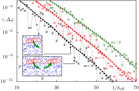
Figure 5: (Color online) Dynamical tunneling rates $\gamma$ (dots), quasi-energy splittings $\Delta\varphi$ (squares), and the prediction of Eq. (7) (lines) vs $1/h_{\text{eff}}$ for the regular states $m\leq 2$. We use the system $\mathcal{D}_{\text{d}}$ (see Sec. IV.1.2). The insets show the phase space with two symmetry-related regular regions (used to determine $\Delta\varphi$) and the phase space with one regular region (used to determine $\gamma$).

Fig. 5 illustrates the strong fluctuations of the splittings $\Delta\varphi_{m}$ (squares) in contrast to the smooth behavior of the tunneling rates $\gamma_{m}$ (dots, lines). As predicted by Eq. (48) one can see in the figure that the splittings fluctuate around the tunneling rates as a function of $1/h_{\text{eff}}$.

This demonstrates that for a quantitative verification of a theory on regular-to-chaotic tunneling the tunneling rates allow for a more precise comparison than tunneling splittings.

III Numerical determination of tunneling rates

To test the theoretical prediction derived in Sec. II we compare its results to numerical rates in Secs. IV and V. In this section we present three alternative methods to numerically compute tunneling rates: (A) opening the system, (B) time evolution of regular states, and (C) evaluating avoided crossings. Figure 6 shows a comparison of the tunneling rates obtained by these three methods for a quantum map. We find excellent agreement between the first two methods while the last approach shows small deviations.

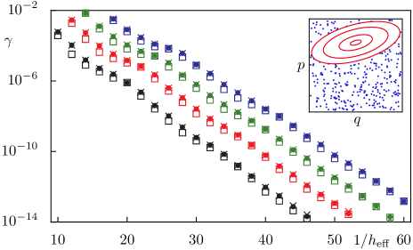
Figure 6: (Color online) Comparison of tunneling rates $\gamma$ obtained by opening the system (dots), time evolution (crosses), and the evaluation of avoided crossings (squares) vs $1/h_{\text{eff}}$. We use the map $\mathcal{D}_{\text{ho}}$ (see Sec. IV.1.1) and consider the regular states $m\leq 3$. The inset shows the phase space of the system.

III.1 Opening the system

The structure of the considered phase space, with one regular island surrounded by the chaotic sea, allows for the determination of tunneling rates by introducing absorption somewhere in the chaotic region of phase space. For quantum maps this can be realized, e.g., by using a non-unitary open quantum map BorGuaShe1991 ; SchTwo2004

$$U^{o}=PUP,$$ (49)

where $P$ is a projection operator onto the complement of the absorbing region. An example is given by a sum of projectors on position eigenstates,

$$P=\sum_{q_{l}}^{q_{r}}|q\rangle\langle q|,$$ (50)

where the regular island is located well inside the interval $[q_{l},q_{r}]$.

While the eigenvalues of $U$ are located on the unit circle the eigenvalues of $U^{o}$ are inside the unit circle as $U^{o}$ is sub-unitary, see Fig. 7. The eigenequation of $U^{o}$ reads

$$U^{o}|\psi_{n}^{o}\rangle=z_{n}|\psi_{n}^{o}\rangle$$ (51)

with eigenvalues

$$z_{n}=\text{e}^{\text{i}\left(\varphi_{n}+\text{i}\frac{\gamma_{n}}{2}\right)}.$$ (52)

The decay rate is characterized by the imaginary part of the quasi-energies in Eq. (52) and one has

$$\gamma_{m}=-2\log|z_{m}|\approx 2(1-|z_{m}|).$$ (53)

In order to obtain the open map $U^{o}$ practically, we quantize the classical map on the cylinder $(q,p)\in[-\infty,\infty]\times[-1/2,1/2]$ with the periodically extended potential $V(q)$. This leads to an infinite dimensional unitary matrix $U$ in position representation ChaShi1986 and we find $U^{o}$ with Eq. (49) using the projector $P$ given by Eq. (50). After the diagonalization of $U^{o}$ we identify the eigenvalues $z_{m}$ of $U^{o}$ close to the unit circle, which correspond to the quasi-bound regular states, and use Eq. (53) to determine the tunneling rates, see Fig. 6 (dots) for an example.

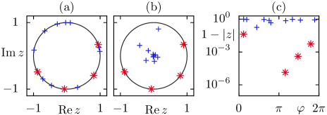
Figure 7: (Color online) (a) The eigenvalues of the unitary quantum map $\mathcal{D}_{\text{ho}}$ (see Sec. IV.1.1) with $h_{\text{eff}}=1/14$ are located on the unit circle. Regular states are marked by red stars, chaotic states by blue plus symbols. (b) The eigenvalues of the open system $U^{o}$ are located inside the unit circle. (c) The distance $1-|z|$ is shown on a logarithmic scale.

If the chaotic region does not contain partial barriers and shows no dynamical localization, it is justified to assume that the probability of escaping the regular island is equal to the probability of leaving through the absorbing regions located in the chaotic sea. Then, the location of the absorbing regions in the chaotic part of phase space has no effect on the decay rates.

In generic systems, however, partial barriers will appear in the chaotic region of phase space. The additional transition through these structures further limits the quantum transport such that the calculated decay through the absorbing region occurs slower than the decay from the regular island to the neighboring chaotic sea. Similarly, dynamical localization in the chaotic region may slow down the decay. The quantitative influence of partial barriers and dynamical localization on the regular-to-chaotic tunneling rates is an open problem for future studies. If necessary we will suppress their influence by moving the absorbing regions closer to the regular island.

III.2 Time evolution

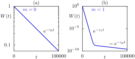
Figure 8: (Color online) Time evolution of a purely regular state for the system $\mathcal{D}_{\text{ho}}$ (see Sec. IV.1.1) with $h_{\text{eff}}=1/14$. We present $W(t)$ vs $t$ obtained by Eq. (54) on a semi-logarithmic scale. (a) For the regular ground state the tunneling rate to the chaotic sea $\gamma_{0}$ is determined by the slope of the numerical data. (b) For the first excited state $m=1$ the slope for small times $t$ determines the tunneling rate $\gamma_{1}$, while for larger times the decay of the ground state $\gamma_{0}$ with a smaller slope is found.

A simple method to obtain a numerical prediction of the tunneling rates for quantum maps is given by the time-evolution of a purely regular state $|\psi_{\text{reg}}^{m}\rangle$ with a non-unitary operator $U^{o}=PUP$. Here $P$ projects onto a region in phase space which includes the regular island. We consider

$$W_{m}(t)=\|P_{\text{reg}}(U^{o})^{t}|\psi_{\text{reg}}^{m}\rangle\|^{2}$$ (54)

for $t\in\mathbb{N}$, which describes the probability of the time-evolved regular state in the regular island at time $t$. At each time step some probability of $|\psi_{\text{reg}}^{m}\rangle$ is absorbed in the chaotic region due to the openness of the quantum map $U^{o}$. Consequently, $W_{m}(t)$ decays exponentially, $W_{m}(t)\approx\text{e}^{-\gamma_{m}t}$, and the tunneling rates $\gamma_{m}$ can be determined by a fit of the numerical data. If $|\psi_{\text{reg}}^{m}\rangle$ contains admixtures from lower excited regular states (with smaller tunneling rates) their decay dominates at times $t\gg 1/\gamma_{m}$. If it contains admixtures from higher excited regular states (with larger tunneling rate) their decay will be seen at small times, see Fig. 8. The computed tunneling rates are in excellent agreement with the results obtained by opening the system, see Fig. 6 (crosses). This method works best for regular states $|\psi_{\text{reg}}^{m}\rangle$ which resemble the corresponding eigenstates of the mixed system $U$ with high accuracy. It is particularly useful for Hilbert spaces of large dimension $N$ where diagonalizing the matrix $U^{o}$ would numerically be very time-consuming.

III.3 Evaluation of avoided crossings

The third method calculates the tunneling rate of a regular state directly from the spectrum of the system. For quantum maps we determine the quasi-energies $\varphi$ under variation of a parameter of the system which leaves the classical dynamics invariant, such as the Bloch phase $\theta_{q}$ or $\theta_{p}$. These phases specify the periodicity conditions on the torus and can be incorporated in the quantization of the map KeaMezRob1999 . Under variation of such a parameter the quasi-energy of the considered regular state $\varphi_{m}$ shows avoided crossings with quasi-energies $\varphi_{\text{ch}}$ of chaotic states, see Fig. 9. These avoided crossings have widths $\Delta\varphi_{\text{ch},m}$. According to degenerate perturbation theory they are related to the matrix elements $v_{\text{ch},m}$ by $\Delta\varphi_{\text{ch},m}=2v_{\text{ch},m}$ and fluctuate depending on the involved chaotic state. The tunneling rate follows from the dimensionless version of Fermi’s golden rule, Eq. (122),

$$\gamma_{m} = \frac{N_{\text{ch}}}{4}\langle|\Delta\varphi_{\text{ch},m}|^{2}\rangle_{\text{ch}},$$ (55)

where $N_{\text{ch}}$ is the number of chaotic states. Note, that the two methods discussed in Secs. III.1 and III.2 determine the tunneling rates $\gamma$ for fixed Bloch phases. Under variation of $\theta_{q}$ or $\theta_{p}$ we observe numerically for these methods that the rates vary by at most a factor of $2$, while Eq. (55) gives an average rate.

The quality of this prediction depends on the number of avoided crossings entering the average in Eq. (55). If only a few avoided crossings are included, the statistical error of the result is large. Note, that for quantum maps with a mean drift in the chaotic sea, such as the systems $\mathcal{D}$ (introduced in Sec. IV.1.1), under variation of the Bloch phases $\theta$ several chaotic states will show avoided crossings with each regular state BerBalTabVor1979 . The results of this method are presented in Fig. 6 (squares) for an example system. We typically obtain tunneling rates which are smaller than the results of the other two methods. While we have no explanation of this behavior, the deviation is smaller than a factor of two, which is sufficient for a comparison to theoretical predictions.

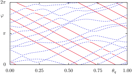
Figure 9: (Color online) Quasi-energies of the quantum map $U$ for the system $\mathcal{D}_{\text{ho}}$ (see Sec. IV.1.1) vs Bloch phase $\theta_{q}$ with $h_{\text{eff}}=1/14$ and $\theta_{p}=0$. Regular states (red solid lines) show avoided crossings with chaotic eigenstates (blue dashed lines).

Also for billiards tunneling rates can be computed by this method. We determine the spectrum under variation of parts of the billiard boundary which leaves the classically regular dynamics unchanged but affects the chaotic dynamics. Quantum mechanically, the eigenenergies of the regular states remain almost unaffected while the eigenenergies of the chaotic states vary strongly, due to the changing density of chaotic states. Hence, avoided crossings of widths $\Delta E_{\text{ch},mn}$ between the considered regular and the chaotic states appear. The tunneling rate is given by Fermi’s golden rule, Eq. (14),

$$\Gamma_{mn}=\frac{2\pi}{\hbar}\frac{\langle|\Delta E_{\text{ch},mn}|^{2}\rho_{\text{ch}}\rangle}{4}\approx\frac{\hbar}{16M}\langle|\Delta E_{\text{ch},mn}|^{2}\mathcal{A}_{\text{ch}}\rangle,$$ (56)

where we average the product of all numerically determined widths $\Delta E_{\text{ch},mn}=2V_{\text{ch},mn}$ and the corresponding density of chaotic states $\rho_{\text{ch}}$, which we approximate by its leading Weyl term, see Sec. II.1.3. Note, that in general it can be difficult to deform a part of the billiard boundary such that the regular dynamics is unchanged while still the numerical methods for the determination of eigenvalues in billiard systems are applicable.

IV Application to quantum maps

In the following we will apply the fictitious integrable system approach, derived in Sec. II, to the prediction of direct regular-to-chaotic tunneling rates in the case of quantum maps and compare the results to numerical rates for different example systems.

IV.1 Designed maps $\mathcal{D}$

Our aim is to introduce kicked systems which can be designed such that their phase space shows one regular island embedded in the chaotic sea, with very small nonlinear resonance chains within the regular island, a negligible hierarchical region, and without relevant partial barriers in the chaotic component. For such a system it is possible to study the direct regular-to-chaotic tunneling process without additional effects caused by these structures.

To this end we define the family of maps $\mathcal{D}$, according to Eq. (21), with an appropriate choice of the functions $T^{\prime}(p)$ and $V^{\prime}(q)$ ShuIke1995 ; SchOttKetDit2001 ; BaeKetMon2005 ; BaeKetLoeSch2008 ; LoeBaeKetSch2010 . For this we first introduce

$$t^{\prime}(p) = \left\{\begin{array}[]{llrcl}\tfrac{1}{2}-(1-2p)&\text{ for }&-\tfrac{1}{2}<&p&<0\\ \tfrac{1}{2}+(1-2p)&\text{ for }&\,0<&p&<\tfrac{1}{2},\end{array}\right.$$ (59)

$$v^{\prime}(q) = \begin{array}[]{llrcl}-rq+Rq^{2}&\hskip 14.51074pt\text{ for }&-\tfrac{1}{2}<&q&<\tfrac{1}{2}\end{array}$$ (61)

with $0<r<2$ and $R\geq 0$. This gives a regular island around $(q,p)=(0,1/4)$. Considering periodic boundary conditions the functions $t^{\prime}(p)$ and $v^{\prime}(q)$ show discontinuities at $p=0,\pm 1/2$ and $q=\pm 1/2$, respectively. In order to avoid these discontinuities we smooth the periodically extended functions $v^{\prime}(q)$ and $t^{\prime}(q)$ with a Gaussian,

$$G(z)=\frac{1}{\sqrt{2\pi\varepsilon^{2}}}\exp\left(-\frac{z^{2}}{2\varepsilon^{2}}\right),$$ (62)

resulting in analytic functions

$$T^{\prime}(p) = \int\limits\text{d}z\,t^{\prime}(z)G(p-z),$$ (63)

$$V^{\prime}(q) = \int\limits\text{d}z\,v^{\prime}(z)G(q-z),$$ (64)

which are periodic with respect to the phase-space unit cell. With this we obtain the maps $\mathcal{D}$ depending on the parameters $r$, $R$, and the smoothing strength $\varepsilon$. The smoothing $\varepsilon$ determines the size of the hierarchical region at the border of the regular island. Tuning the parameters $r$ and $R$ one can find situations, where all nonlinear resonance chains inside the regular island are small.

IV.1.1 Map $\mathcal{D}_{\text{ho}}$ with harmonic oscillator-like island

For $R=0$ both functions $v^{\prime}(q)$ and $t^{\prime}(p)$ are linear in $q$ and $p$, respectively. In this case we find a harmonic oscillator-like regular island with elliptic invariant tori and constant rotation number. We choose the parameters $r=0.46$, $R=0$, $\varepsilon=0.005$ and label the resulting map by $\mathcal{D}_{\text{ho}}$. Its phase-space is shown in the insets of Fig. 10. Numerically, we determine tunneling rates by introducing absorbing regions at $|q|\geq 1/2$, as described in Sec. III.1. In order to apply the fictitious integrable system approach we use the Hamiltonian of a harmonic oscillator as $H_{\text{reg}}$. It is squeezed and tilted according to the linearized dynamics in the vicinity of the stable fixed point located at the center of the regular island. Its eigenfunctions $|\psi_{\text{reg}}^{m}\rangle$ are analytically known, see Appendix B.

Figure 10(a) shows the numerically evaluated prediction of Eq. (7) compared to numerical tunneling rates. We find excellent agreement over more than $10$ orders of magnitude in $\gamma$. In the regime of large tunneling rates small deviations occur which can be attributed to the influence of the chaotic sea on the regular states: These states are located on quantizing tori close to the border of the regular island and are affected by the regular-to-chaotic transition region. However, the deviations in this regime are smaller than a factor of two.

Figure 10(b) shows the results of Eq. (29), which are obtained by approximating $U_{\text{reg}}$ by a kicked system, $\widetilde{U}_{\text{reg}}=U_{\widetilde{V}}U_{T}$, again using the analytically given $|\psi_{\text{reg}}^{m}\rangle$. These results are still in excellent agreement with the numerical rates (solid lines). In Eq. (30) the sum over the positions is replaced by an integral, which explains the small deviations to the results of Eq. (29), see Fig. 10(b) (dashed lines). These deviations vanish in the semiclassical limit.

Finally, in Fig. 10(c) we compare the results of the semiclassical prediction, Eq. (43), to the numerical rates. Due to the approximations performed in the derivation of this formula stronger deviations are visible in the regime of large tunneling rates while the agreement in the semiclassical regime is still excellent.

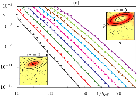
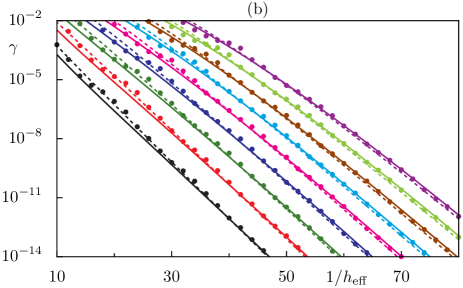
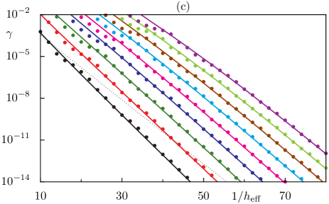
Figure 10: (Color online) Numerical tunneling rates (dots) for $m\leq 8$ for the map $\mathcal{D}_{\text{ho}}$ with a harmonic oscillator-like island. (a) Comparison with Eq. (7) (lines). The insets show Husimi functions of the regular states for the quantum numbers $m=0$ and $m=5$ at $1/h_{\text{eff}}=30$ and the classical phase space of the system. (b) Comparison with Eqs. (29) (solid lines) and (30) (dashed lines). (c) Comparison with Eq. (43) (solid lines). The prediction of Refs. PodNar2003 ; She2005 , Eq. (65), for $m=0$ with a fitted prefactor is shown (dotted line).

In Refs. PodNar2003 ; She2005 a prediction was derived for the tunneling rate of the regular ground state,

$$\gamma_{0}=c\frac{\Gamma(\alpha,4\alpha)}{\Gamma(\alpha,0)},$$ (65)

where $\Gamma$ is the incomplete gamma function, $\alpha=A_{\text{reg}}/h_{\text{eff}}$, and $c$ is a constant. Equation (65) can be approximated semiclassically SchEltUll2005 , $\alpha\to\infty$, leading to

$$\gamma_{0}\propto\frac{1}{\sqrt{\alpha}}\text{e}^{-\alpha(3-\ln 4)}.$$ (66)

Figure 10(c) shows the comparison of Eq. (65) (dotted line) to the numerical rates for the map $\mathcal{D}_{\text{ho}}$. Especially in the semiclassical regime strong deviations are visible. The factor $2$ which appears in the exponent of Eq. (43) is more accurate than the factor $3-\ln 4$ in Eq. (66).

IV.1.2 Map $\mathcal{D}_{\text{d}}$ with deformed island

In generic systems the regular island has a non-elliptic shape and the rotation number of regular tori changes from the center of the regular region to its border with the chaotic sea. Such a situation can be achieved for the family of maps $\mathcal{D}$ with the parameter $R\neq 0$. For most combinations of the parameters $r$ and $R$ resonance structures appear inside the regular island. They limit the $h_{\text{eff}}$-regime in which the direct regular-to-chaotic tunneling process dominates. Hence, we choose a situation in which the nonlinear resonances are small such that their influence on the tunneling process is expected only at large $1/h_{\text{eff}}$. For this we use $r=0.26$, $R=0.4$, $\varepsilon=0.005$ and label the resulting map with a deformed island by $\mathcal{D}_{\text{d}}$, see the inset in Fig. 11 for its phase space.

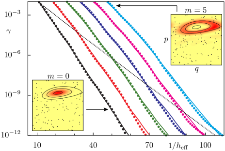
Figure 11: (Color online) Dynamical tunneling rates from a regular island to the chaotic sea for the map $\mathcal{D}_{\text{d}}$. Numerical rates (dots) and prediction following from Eq. (7) (lines) vs $1/\hbar_{\text{eff}}$ for quantum numbers $m\leq 5$. The insets show Husimi representations of the regular states $m=0$ and $m=5$ at $1/h_{\text{eff}}=50$. The prediction of Refs. PodNar2003 ; She2005 , Eq. (65), for $m=0$ with a fitted prefactor is shown (dotted line).

We determine the fictitious integrable system $H_{\text{reg}}$ by means of the Lie-transformation method described in Sec. II.2. It is then quantized and its eigenfunctions are determined numerically. Figure 11 shows a comparison of the numerically evaluated prediction of Eq. (7) (solid lines) to numerical tunneling rates (dots) yielding excellent agreement for $\gamma\gtrsim 10^{-11}$. For smaller values of $\gamma$ deviations occur due to resonance-assisted tunneling which is caused by a small $10$:$1$ resonance chain. Similar to the case of the harmonic oscillator-like island the fictitious integrable system $U_{\text{reg}}$ can be approximated by a kicked system $U_{\text{reg}}\approx U_{\widetilde{V}}U_{\text{T}}$ using $\widetilde{V}(q)=-rq^{2}/2+Rq^{3}/3$. Hence, Eqs. (29) and (30) can be evaluated giving similarly good agreement (not shown). The prediction of Eq. (65) PodNar2003 ; She2005 (dotted line) shows large deviations to the numerical rates.

IV.1.3 Map $\mathcal{D}_{\text{wc}}$ with weakly chaotic dynamics

In Ref. SheFisGuaReb2006 the dynamical tunneling process from one regular island to the chaotic sea in a system with weakly chaotic dynamics was investigated. Here, tunneling can occur to regions in phase space which are far away from the border of the regular island with the chaotic sea. We show that also in this situation, which we believe to be non-generic, the fictitious integrable system approach can be applied. Its results will be compared to the WKB prediction of Ref. SheFisGuaReb2006 .

A system with weakly chaotic dynamics can be modeled by the example systems $\mathcal{D}$. We choose $r=0.05$, $R=0.1$, and $\varepsilon=0.005$, consider the extended phase space $(q,p)\in[-1,1]\times[-1/2,1/2]$, and label the resulting map by $\mathcal{D}_{\text{wc}}$. Its phase space is shown in the upper inset of Fig. 12.

In order to apply the fictitious integrable system approach we use the Lie-transformation method, as described in Sec. II.2, to obtain the fictitious integrable system $H_{\text{reg}}$. As the system $\mathcal{D}_{\text{wc}}$ is only weakly driven, due to the small parameters $r$ and $R$, it is sufficient to consider the zeroth order of the Lie expansion which has no mixed terms containing $q$ and $p$ simultaneously. The resulting integrable approximation

$$H_{\text{reg}}(q,p)=\frac{p^{2}}{2}+W(q),$$ (67)

describes the dynamics in a potential $W(q)=\omega^{2}q^{2}/2-Rq^{3}/6$ with $\omega=\sqrt{r/2}$, see the lower inset in Fig. 12.

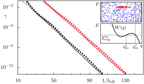
Figure 12: (Color online) Dynamical tunneling rates from a regular island to the chaotic sea for the weakly chaotic system $\mathcal{D}_{\text{wc}}$. We compare numerical rates (dots) and the prediction following from Eq. (7) (solid lines) and Eq. (68) SheFisGuaReb2006 (dashed lines) vs $1/h_{\text{eff}}$ for $m=0$ and $m=1$. The upper inset shows the phase space of the system, where the absorbing regions are indicated in gray. In the lower inset the approximate one-dimensional potential $W(q)$ used in Eq. (68) is presented with the inner (outer) turning point $q_{m}^{\text{i}}$ ($q_{m}^{\text{o}}$) at energy $E_{\text{reg}}^{m}$.

In Ref. SheFisGuaReb2006 it was shown that for such a weakly chaotic system regular-to-chaotic tunneling rates can be predicted by one-dimensional tunneling under the energy barrier of the potential $W(q)$. For the tunneling rates one finds

$$\gamma_{m}\approx\frac{\omega_{m}}{2\pi}\exp\left(-\frac{2}{\hbar_{\text{eff}}}\int\limits_{q_{m}^{\text{i}}}^{q_{m}^{\text{o}}}|p(q,E_{\text{reg}}^{m})|\,\text{d}q\right)$$ (68)

where $p(q,E_{\text{reg}}^{m})=\sqrt{2E_{\text{reg}}^{m}-\omega^{2}q^{2}+Rq^{3}/3}$, $q_{m}^{\text{i}}$ denotes the right classical turning point inside the potential well, $q_{m}^{\text{o}}$ is the turning point outside the potential well, and $\omega_{m}$ is the oscillation period on the $m$th quantizing torus. The eigenenergies $E_{\text{reg}}^{m}$ can be calculated using the Bohr-Sommerfeld quantization $\oint p(q,E_{\text{reg}}^{m})\,\text{d}q=h_{\text{eff}}(m+1/2)$. For the system $\mathcal{D}_{\text{wc}}$ the right turning point $q_{m}^{\text{o}}$ is located far away from the regular island. Tunneling occurs to the region with $q>q_{m}^{\text{o}}$ deep inside the weakly chaotic sea and not to the neighborhood of the regular island, as for the other examples considered in this paper.

In Fig. 12 we compare the numerically evaluated prediction of Eq. (7) (solid lines) to the result of Eq. (68) (dashed lines) and numerical rates (dots), which are determined by absorbing regions at $|q|\geq 1$. We find good agreement.

Note, that for the weakly chaotic system $\mathcal{D}_{\text{wc}}$ the purely regular states $|\psi_{\text{reg}}^{m}\rangle$ of $H_{\text{reg}}$ show the correct tunneling tails far beyond the regular island including the outer turning point $q_{m}^{\text{o}}$. Moreover, the semiclassical evaluation of Eq. (8), presented in Sec. II.3, can be performed. This leads to Eq. (42) which has the same exponential term as Eq. (68) but a different prefactor.

We want to emphasize that generically regular-to-chaotic tunneling cannot be described by Eq. (68), as the integrable approximation $H_{\text{reg}}$ is not of the form Eq. (67).

IV.2 Standard map

The paradigmatic model of an area preserving map is the standard map Chi1979 , defined by Eq. (21) with the functions

$$T^{\prime}(p) = p,$$ (69)

$$V^{\prime}(q) = \frac{\kappa}{2\pi}\sin(2\pi q).$$ (70)

For $\kappa$ between $2.5$ and $3.0$ one has a large generic regular island with a relatively small hierarchical region surrounded by a $4$:$1$ resonance chain, see the inset in Fig. 13.

When determining tunneling rates numerically by introducing absorbing regions at $|q|\geq 1/2$ we find strong fluctuations as a function of $h_{\text{eff}}$, presumably caused by partial barriers. Using absorption at $|q|\geq 1/4$, which is closer to the island, we find smoothly decaying tunneling rates (dots in Fig. 13).

Evaluating Eq. (7) for $\kappa=2.9$ gives reasonable agreement with these numerical rates with deviations up to a factor of $5$, see Fig. 13 (solid lines). Here we determine $H_{\text{reg}}$ using the method based on the frequency map analysis as the Lie transformation is not able to reproduce the dynamics within the regular island of $U$, see Sec. II.2. With increasing order $K$ of the expansion series of $H_{\text{reg}}$ the tunneling rates following from Eq. (7) diverge, see Fig. 4(b). Hence, for the predictions in Fig. 13 we choose $K=2$ which is the largest order before the divergence starts to set in. Note, that at such small order $K$ the accuracy of $H_{\text{reg}}$ within the regular region of $U$ is inferior compared to the examples discussed before. Hence, in Eq. (7) the state $U|\psi_{\text{reg}}^{m}\rangle$ has small contributions of other purely regular states $|\psi_{\text{reg}}^{n}\rangle$ in the regular island. These contributions are compensated by the application of the projector $P_{\text{ch}}$. However, this projector depends on the number of regular states $N_{\text{reg}}$, which grows in the semiclassical limit. If $N_{\text{reg}}$ increases by one, $P_{\text{reg}}$ suddenly projects onto a larger region in phase space. This explains the steps of the theoretical prediction, Eq. (7), visible in Fig. 13. How to improve $H_{\text{reg}}$ and the projector $P_{\text{ch}}$ is an open question.

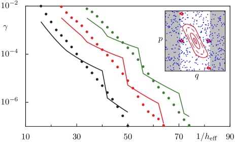
Figure 13: (Color online) Tunneling rates for the standard map ($\kappa=2.9$) for $m\leq 2$ vs $1/h_{\text{eff}}$. Prediction of Eq. (7) (lines) and numerical rates (dots), obtained using absorbing regions at $|q|\geq 1/4$ (gray-shaded area of the inset).

IV.3 Map $\mathcal{D}_{\text{rs}}$ with a regular stripe

Another designed kicked system was introduced in Refs. ShuIke1995 ; ShuIke1998 ; IshTanShu2007 ; IshTanShu2009 . Here the regular region consists of a stripe in phase space, see the inset in Fig. 14. In our notation the mapping $\mathcal{D}_{\text{rs}}$, Eq. (21), is specified by the functions

$$V^{\prime}(q) = -\frac{1}{2\pi}(8\pi aq+d_{1}-d_{2}$$ (71)

$$+\frac{1}{2}[8\pi aq-\omega+d_{1}]\tanh[b(8\pi q-q_{d})]$$

$$+\frac{1}{2}[-8\pi aq+\omega+d_{2}]\tanh[b(8\pi q+q_{d})]),\;\;\;$$

$$T^{\prime}(p) = -\frac{K}{8\pi}\sin(2\pi p)$$ (72)

with parameters $a=5$, $b=100$, $d_{1}=-24$, $d_{2}=-26$, $\omega=1$, $q_{d}=5$, and $K=3$. The kinetic energy $T(p)$ is periodic with respect to the phase space unit cell.

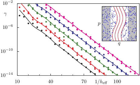
Figure 14: (Color online) Dynamical tunneling rates from a regular stripe to the chaotic sea for the map $\mathcal{D}_{\text{rs}}$. We compare numerical rates (dots) and the prediction following from Eq. (7) (lines) vs $1/h_{\text{eff}}$ for the quantum numbers $|m|\leq 4$. The inset shows the phase space of the system. The numerical rates are obtained using absorbing regions at $|q|\geq 1/4$ (gray-shaded area of the inset).

The resulting map $\mathcal{D}_{\text{rs}}$ is similar to the system $\mathcal{D}_{\text{ho}}$ as it also destroys the integrable region by smoothly changing the function $V^{\prime}(q)$ at $|q|=q_{d}/(8\pi)$. For $|q|<q_{d}/(8\pi)$ the potential term is almost linear while it tends to the standard map for $|q|>q_{d}/(8\pi)$. The parameter $b$ determines the width of the transition region. In Ref. IshTanShu2007 this map is used to study the evolution of a wave packet initially started in the regular region by means of complex paths. We now predict direct regular-to-chaotic tunneling rates with Eq. (7). The fictitious integrable system $U_{\text{reg}}$ is determined by continuing the dynamics within $|q|<q_{d}/(8\pi)$ to the whole phase space. It is given as a kicked system, Eq. (21), defined by the functions

$$\widetilde{V}^{\prime}(q) = -\frac{1}{2\pi}\left(\omega+\frac{d_{1}}{2}-\frac{d_{2}}{2}\right),$$ (73)

$$T^{\prime}(p) = -\frac{K}{8\pi}\sin(2\pi p).$$ (74)

When determining tunneling rates numerically using absorbing regions at $|q|\geq 1/2$ we find strong fluctuations as a function of $h_{\text{eff}}$, similar to the standard map. Choosing $|q|\geq 1/4$ for the opening, which is closer to the regular stripe, we find smoothly decaying tunneling rates (dots in Fig. 14). Their comparison with the numerical evaluated prediction of Eq. (7) shows excellent agreement, see Fig. 14 (lines).

Note, that due to the symmetry of the map there are always two regular states with comparable tunneling rates except for the ground state $m=0$. These two states are located symmetrically around the center of the regular stripe. While the prediction, Eq. (7), is identical for both of these states, the numerical results differ slightly due to the different chaotic dynamics in the vicinity of the left and right borders of the regular region.

V Application to billiards

Billiards play a central role in both experimental and theoretical studies in quantum chaos. They are dynamical systems given by a point particle of mass $M$ which moves with constant velocity inside a domain $\Omega\in\mathbb{R}^{2}$ which we assume to be compact. The particle is elastically reflected at the boundary $\partial\Omega$ such that the angle of incidence equals the angle of reflection. While there are only a few integrable and completely chaotic billiards, the majority shows a mixed phase space consisting of regions of regular and chaotic dynamics. Quantum mechanically, billiards are described by the time-independent Schrödinger equation (in units $\hbar=2M=1$ used in this section)

$$-\Delta\psi_{n}(\boldsymbol{q})=E_{n}\psi_{n}(\boldsymbol{q}),\quad\boldsymbol{q}\in\Omega$$ (75)

with the Dirichlet boundary condition $\psi_{n}(\boldsymbol{q})=0$, $\boldsymbol{q}\in\partial\Omega$. In Eq. (75) $\Delta$ denotes the Laplace operator in two dimensions. Equation (75) is identical to the eigenvalue problem of the two-dimensional Helmholtz equation which for example describes electro-magnetic modes in a microwave cavity. This equivalence allows for the simulation of quantum billiards by experiments using microwave cavities StoSte1990 ; Sri1991 ; GraHarLenLewRanRicSchWei1992 ; SteSto1992 ; AltBaeDemGraHofRehRic1998 .

The state of a particle is described by a wave function $\psi(\boldsymbol{q})\in L^{2}(\Omega)$ in position representation, where $L^{2}(\Omega)$ is the Hilbert space of square integrable functions on $\Omega$. Due to the compactness of $\Omega$ the eigenvalues $\{E_{n}\}$ are discrete and can be ordered as $0\leq E_{1}\leq E_{2}\leq E_{3}\leq\cdots$. The eigenfunctions can be chosen real and form an orthonormal basis on $L^{2}(\Omega)$. In contrast to the case of quantum maps discussed in Sec. IV one gets infinitely many eigenvalues and eigenfunctions. There are only a few billiard systems, whose eigenfunctions are analytically known, e.g., the rectangular, circular, and elliptical billiard. Usually an analytical solution of Eq. (75) is not possible.

The determination of tunneling rates for two-dimensional billiard systems is of current interest. It is relevant, e.g., in the context of light emission in optical microcavities WieHen2006 ; WieHen2008 ; ShiHarFukHenSasNar2010 ; YanLeeMooLeeKimDaoLeeAn2010 , flooding of regular states BaeKetMon2005 ; BaeKetMon2007 ; Bit2010 and conductance properties of electrons in disordered wires with a magnetic field FeiBaeKetRotHucBur2006 ; FeiBaeKetBurRot2009 . Previous theoretical predictions of tunneling rates BarBet2007 or energy-splittings DorFri1995 ; FriDor1998 in billiards required additional free parameters.

We apply the fictitious integrable system approach in order to determine direct regular-to-chaotic tunneling rates for billiards. For this we employ Eqs. (13) and (14), where in the following we omit the tilde of the non-orthogonal chaotic states $\widetilde{\psi}_{\text{ch}}$ and label the corresponding dimensionless matrix elements and tunneling rates by $v_{\text{ch},mn}$ and $\gamma_{mn}$, respectively. For the chaotic states entering in Eq. (13) we employ random wave models Ber1977 such that the average in Eq. (14) becomes an ensemble average over the different realizations of the random wave model. From this we obtain explicit analytical predictions for the mushroom billiard BaeKetLoeRobVidHoeKuhSto2008 , the annular billiard, two-dimensional nanowires with one-sided surface disorder, and optical microcavities BaeKetLoeWieHen2009 .

V.1 Mushroom billiard

We consider the desymmetrized mushroom billiard Bun2001 , see Fig. 15(a), characterized by the radius $R$ of the quarter circular cap, the stem width $a$, and the stem height $l$. This billiard is of great current interest VidStoRobKuhHoeGro2007 ; BarBet2007 ; AltMotKan2005 ; TanShu2006 ; DieFriMisRicSch2007 due to its sharply separated regular and chaotic regions in phase space. The regular trajectories show whispering-gallery motion and do not cross the small quarter circle of radius $a$. Each trajectory which crosses this curve is chaotic, see Fig. 15(c). There is no hierarchical regular-to-chaotic transition region and there appear no resonance chains inside the regular island. Hence, for this billiard resonance-assisted tunneling does not occur and the direct regular-to-chaotic tunneling process is relevant for all energies $E$. The application of the fictitious integrable system approach to the mushroom billiard leads to the explicit analytical formula (93), which was obtained in Ref. BaeKetLoeRobVidHoeKuhSto2008 , where it was successfully compared to experimental data.

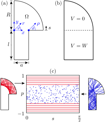
Figure 15: (Color online) (a) Schematic picture of the mushroom billiard, with cap radius $R$, stem width $a$, and stem height $l$, showing the two coordinate systems used in the theoretical derivation of the direct regular-to-chaotic tunneling rates. (b) Auxiliary billiard $H_{\text{reg}}^{W}$. (c) Poincaré section at the quarter-circle boundary (relative tangential momentum $p$ vs arclength $s$) showing regular and chaotic regions with illustrations of trajectories.

V.1.1 Derivation of tunneling rates

In order to predict tunneling rates for the mushroom billiard we review the derivation BaeKetLoeRobVidHoeKuhSto2008 starting from Eqs. (13) and (14). First we construct a fictitious integrable system $H_{\text{reg}}$, determine its eigenstates $\psi_{\text{reg}}^{mn}(\boldsymbol{q})$, and find a model for the chaotic states $\psi_{\text{ch}}(\boldsymbol{q})$. In the following analysis we set $R=1$. A natural choice for the regular system $H_{\text{reg}}$ is the quarter-circle billiard. Its eigenfunctions are analytically known

$$\psi_{\text{reg}}^{mn}(r,\varphi)=N_{mn}J_{m}(j_{mn}r)\sin(m\varphi),$$ (76)

in polar coordinates $(r,\varphi)$. They are characterized by the radial $(n=1,2,\dots)$ and the azimuthal $(m=2,4,\dots)$ quantum numbers. As we are considering the quarter-circle billiard $m$ is allowed to take even values only. Here $J_{m}$ denotes the $m$th Bessel function, $j_{mn}$ the $n$th root of $J_{m}$, $N_{mn}=\sqrt{8/\pi}/J_{m-1}(j_{mn})$ accounts for the normalization, and $E_{mn}=j_{mn}^{2}$ are the eigenenergies. Among the regular states of the quarter-circle billiard we will consider only those which concentrate on regular tori of the mushroom billiard with angular momentum $p_{mn}=m/j_{mn}>a$.

We use the Hamiltonian $H$ of the mushroom and $H_{\text{reg}}$ of the quarter-circle billiard in Eq. (13) to determine the coupling between the regular and the chaotic states. An infinite potential difference $H-H_{\text{reg}}=-\infty$ occurs, while $\psi_{\text{reg}}^{mn}=0$ in the stem of the mushroom for $y<0$. In order to avoid the undefined product $(H-H_{\text{reg}})\psi_{\text{reg}}^{mn}$ we introduce a finite potential at $y\leq 0$, see Fig. 15(b),

$$H_{\text{reg}}^{W}(\boldsymbol{q},\boldsymbol{p}) = \boldsymbol{p}^{2}+V(\boldsymbol{q})$$ (77)

$$V(\boldsymbol{q}) = \left\{\begin{array}[]{ll}0&\quad\text{for }x^{2}+y^{2}\leq 1,\;x,\,y>0\\ W&\quad\text{for }y\leq 0,\;0\leq x\leq 1\\ \infty&\quad\text{otherwise}\end{array}\right.$$ (81)

and consider the limit $W\to\infty$ in which the quarter-circle billiard is recovered. For finite $W$ the regular eigenfunctions $\psi_{\text{reg},W}^{mn}(\boldsymbol{q})$ of $H_{\text{reg}}^{W}$ decay into the region $y<0$. To describe this decay we make the following ansatz

$$\psi_{\text{reg},W}^{mn}(x,y)=\psi_{\text{reg},W}^{mn}(x,y=0)\text{e}^{\lambda y},$$ (82)

where $\lambda$ depends on $W$ via the Schrödinger equation as

$$-\lambda^{2}+W=E_{mn}^{W}.$$ (83)

Since the regular eigenfunctions $\psi_{\text{reg},W}^{mn}$ and their derivatives have to be continuous at $y=0$ we obtain

$$\lambda=\frac{\partial_{y}\psi_{\text{reg},W}^{mn}(x,y=0)}{\psi_{\text{reg},W}^{mn}(x,y=0)}.$$ (84)

Evaluating Eq. (13) for the coupling matrix elements one finds

$$v_{\text{ch},mn} = \lim_{W\to\infty}\int\limits_{0}^{a}\text{d}x\int\limits_{-l}^{0}\text{d}y\,\psi_{\text{ch}}(x,y)(-W)\psi_{\text{reg},W}^{mn}(x,y)\quad\;\;$$ (85)

$$= -\lim_{W\to\infty}\int\limits_{0}^{a}\text{d}x\int\limits_{-l}^{0}\text{d}y\,\psi_{\text{ch}}(x,y)\frac{W}{\lambda}\text{e}^{\lambda y}\partial_{y}\psi_{\text{reg},W}^{mn}(x,0)$$ (86)

In the last equation the term $W\text{e}^{\lambda y}/\lambda$ appears, which in the limit $W\to\infty$ gives for $y\leq 0$

$$\frac{W}{\lambda}\text{e}^{\lambda y}=\frac{W}{\sqrt{W-E_{mn}^{W}}}\text{e}^{\sqrt{W-E_{mn}^{W}}y}\to 2\delta(y),$$ (87)

where we use Eq. (83) and that $E_{mn}^{W}$ remains bounded. For the coupling matrix elements, Eq. (86), we obtain

$$v_{\text{ch},mn} = -\int\limits_{0}^{a}\text{d}x\,\psi_{\text{ch}}(x,y=0)\partial_{y}\psi_{\text{reg}}^{mn}(x,y=0).\quad$$ (88)

Due to the limiting process only an integration along the line $y=0$ remains which connects the quarter circle billiard to the stem of the mushroom. Equation (88) contains the derivative of the regular wave function perpendicular to this line. The largest contribution of the integral is close to the corner of the mushroom at $x=a$, as the derivative of the regular eigenfunctions $\partial_{y}\psi_{\text{reg}}^{mn}$ decays toward $x=0$. Inserting the regular states, Eq. (76), one finds

$$v_{\text{ch},mn} = -N_{mn}\int\limits_{0}^{a}\text{d}x\,\psi_{\text{ch}}(x,y=0)\frac{m}{x}J_{m}(j_{mn}x).\quad$$ (89)

In order to evaluate Eq. (89) we use a random wave description to model the chaotic states $\psi_{\text{ch}}(\boldsymbol{q})$. It has to respect the Dirichlet boundary conditions in the vicinity of the corner at $x=a$. For this random wave model we use polar coordinates $\boldsymbol{q}=(\rho,\vartheta)$ as introduced in Fig. 15(a) such that the corner of angle $3\pi/2$ is located at $(0,0)$. The Dirichlet boundary conditions at this corner are accounted for using Leh1959

$$\psi_{\text{ch}}(\rho,\vartheta)=\sqrt{\frac{8}{3\mathcal{A}_{\text{ch}}}}\sum_{s=1}^{\infty}c_{s}J_{\frac{2s}{3}}(k\rho)\sin\left(\frac{2s}{3}\vartheta\right)$$ (90)

in which $x-a=\rho\cos(\vartheta)$ and $y=\rho\sin(\vartheta)$. The coefficients $c_{s}$ are independent Gaussian random variables with mean zero, $\langle c_{s}\rangle=0$, and unit variance, $\langle c_{s}c_{t}\rangle=\delta_{st}$. Equation (90) fulfills the Schrödinger equation at energy $E=k^{2}$ and the prefactor is chosen such that $\langle|\psi_{\text{ch}}(\rho,\vartheta)|^{2}\rangle=1/\mathcal{A}_{\text{ch}}$ holds far away from the corner. Note, that we do not require these chaotic states to decay into the regular island, as Eq. (89) is an integral along a line of the billiard where the phase space is fully chaotic. Near the boundary, but far away from the corner, $\langle|\psi_{\text{ch}}|^{2}\rangle$ recovers the behavior $1-J_{0}(2k|x|)$ BaeSchSti1998 ; Ber2002 . Inserting Eq. (90) into Eq. (89) at energy $E_{mn}=j_{mn}^{2}$ and $\vartheta=\pi$, we obtain the coupling matrix elements

$$v_{\text{ch},mn} = -N_{mn}\sqrt{\frac{8}{3\mathcal{A}_{\text{ch}}}}\sum_{s=1}^{\infty}c_{s}\sin\left(\frac{2s}{3}\pi\right)$$ (91)

$$\cdot\int\limits_{0}^{a}J_{\frac{2s}{3}}(j_{mn}[a-x])\frac{m}{x}J_{m}(j_{mn}x)\,\text{d}x,$$

where terms with $s$ a multiple of $3$ vanish. Using these matrix elements in Fermi’s golden rule, Eq. (14), gives a prediction of the tunneling rates

$$\gamma_{mn}=m^{2}N_{mn}^{2}\sideset{}{{}^{\prime}}{\sum}_{s=1}^{\infty}\left[\int\limits_{0}^{a}\frac{\text{d}x}{x}\,J_{\frac{2s}{3}}(j_{mn}(a-x))J_{m}(j_{mn}x)\right]^{2}.$$ (92)

The prime at the summation indicates that the sum over $s$ excludes all multiples of three. The remaining integral can be solved analytically (AbrSte1970, , Eq. 11.3.40), leading to the final result

$$\gamma_{mn}=\frac{8}{\pi}\sideset{}{{}^{\prime}}{\sum}_{s=1}^{\infty}\frac{J_{m+\frac{2s}{3}}(j_{mn}a)^{2}}{J_{m-1}(j_{mn})^{2}}.$$ (93)

This gives a prediction of direct regular-to-chaotic tunneling rates of any regular state $\psi_{\text{reg}}^{mn}$ to the chaotic sea in the mushroom billiard. The sum has its dominant contribution for $s=1$ and evaluating Eq. (93) up to $s\leq 2$ gives sufficiently accurate predictions.

It is worth to remark that a very plausible estimate of the tunneling rate is given by the averaged square of the regular wave function on a circle with radius $a$, i.e. the boundary to the fully chaotic phase space, yielding $\gamma_{mn}^{0}=N_{mn}^{2}J_{m}(j_{mn}a)^{2}/2$. Surprisingly, it is just about a factor of $2$ larger for the parameters we studied. In Ref. BarBet2007 a related quantity is proposed, given by the integral of the squared regular wave function over the quarter circle with radius $a$. This quantity, however, is too small by a factor of order $100$ for the parameters under consideration.

V.1.2 Comparison with numerical rates

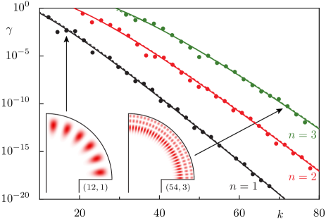
Figure 16: (Color online) Tunneling rates of regular states with quantum numbers $n\leq 3$ vs $k$ for $a=0.5$ comparing the prediction of Eq. (93) (solid lines) and numerical rates (dots). The insets show the regular eigenfunctions $\psi_{\text{reg}}^{12,1}$ and $\psi_{\text{reg}}^{54,3}$ (as indicated by labels). In addition the asymptotic prediction of Eq. (98) is presented (dashed lines).

The eigenvalues and eigenfunctions of the mushroom billiard are determined by numerically solving the Schrödinger equation. The improved method of particular solutions BetTre2005 ; BarBet2007 allows a determination of the energies $E$ with a relative error $\approx 10^{-14}$. We analyze the widths $\Delta E_{\text{ch},mn}$ of avoided crossings between a given regular state and typically $30$ chaotic states under variation of the height $l$ of the stem, starting with $l=0.3$. From Eq. (56), $\gamma\approx\langle|\Delta E_{\text{ch},mn}|^{2}\mathcal{A}_{\text{ch}}\rangle/8$, we deduce the tunneling rate where we use $\mathcal{A}_{\text{ch}}=la+[\arcsin(a)+a\sqrt{1-a^{2}}]/2$ BaeKetLoeRobVidHoeKuhSto2008 as derived in Appendix C. Note, that some pairs of regular states are very close in energy, e.g., $E_{20,1}-E_{16,2}\approx 10^{-4}$, such that their avoided crossings with a chaotic state overlap, making a numerical determination of the smaller tunneling rate unfeasible within the presented approach.

Figure 16 shows the numerical tunneling rates $\gamma_{mn}$ for fixed radial quantum number $n=1,2,3$ and increasing azimuthal quantum number $m$ for $a=0.5$. It is compared to the theoretical prediction, Eq. (93), which is connected for fixed $n$ and increasing $m$ by straight lines, giving rise to an apparently smooth curve. We find excellent agreement for tunneling rates $\gamma_{mn}$ over $18$ orders of magnitude. The small oscillations which appear in the numerical rates on top of the exponential decay might be related to the two-level approximation for avoided crossings which we use for the numerical determination of the tunneling rates.

To further test the prediction we determine the tunneling rate of the regular state $(m,n)=(30,1)$ under variation of the stem width $a$. The results presented in Fig. 17 show a decrease of this tunneling rate which appears faster than exponential with $1-a$. Again we find excellent agreement to numerical rates. Note, that the accuracy of the numerical method used for determining eigenenergies of the mushroom is best for $a\approx 0.5$ and declines for larger or smaller $a$.

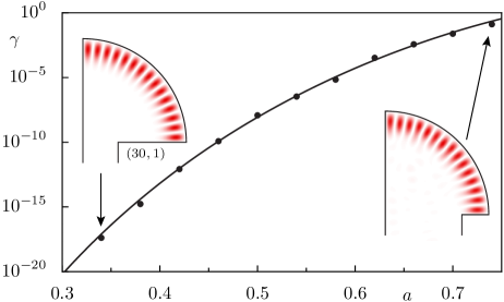
Figure 17: (Color online) Tunneling rates of the regular state $\psi_{\text{reg}}^{30,1}$ vs the stem width $a$. We compare the prediction of Eq. (93) (solid lines) and numerical rates (dots). The insets show the regular eigenfunction $\psi_{\text{reg}}^{30,1}$ at $a=0.34$ and $a=0.74$.

Another interesting question is how the tunneling rates from a given classical torus behave. For this we consider a sequence of regular states $(m,n)$ which semiclassically localize on a torus characterized by an angular momentum $p_{t}>a$. For each $n$ we choose $m$ such that $p_{mn}=m/j_{mn}\approx p_{t}$. The resulting behavior of the tunneling rates is presented in Fig. 18 for $p_{t}=0.6$ and $p_{t}=0.8$. A comparison of these predictions to numerical rates shows excellent agreement.

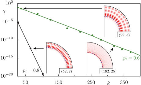
Figure 18: (Color online) Tunneling rates of regular states localized closest to a classical torus of angular momentum $p_{t}=0.8$ and $p_{t}=0.6$ vs $k$ for $a=0.5$. We compare the prediction of Eq. (93) (solid lines) and numerical rates (dots). The insets show the regular eigenfunctions $\psi_{\text{reg}}^{52,2}$ close to $p_{t}=0.8$ and $\psi_{\text{reg}}^{22,3}$, $\psi_{\text{reg}}^{192,25}$ close to $p_{t}=0.6$.

For fixed azimuthal quantum number $m$ and increasing radial quantum number $n$ the tunneling rates increase. This behavior is presented in Fig. 19. Again we find good agreement between the predictions of Eq. (93) and numerical rates.

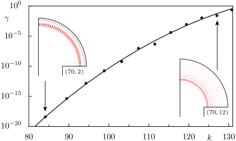
Figure 19: (Color online) Tunneling rates of regular states with quantum number $m=70$ vs $k$ for $a=0.5$ comparing the prediction of Eq. (93) (solid lines) and numerical rates (dots). The insets show the regular eigenfunctions $\psi_{\text{reg}}^{70,2}$ and $\psi_{\text{reg}}^{70,12}$.

V.1.3 Approximation

Let us now approximate Eq. (93) for $m\gg n$ and large wave numbers $k$ in order to understand the exponential behavior of the tunneling rates, which is visible in Figs. 16 and 18 with increasing $k$. First we consider the numerator of the leading term $s=1$ in Eq. (93) and use Ref. (AbrSte1970, , Eq. 9.1.63) for non-integer arguments of the Bessel function

$$J_{m+\frac{2}{3}}(j_{mn}a)\leq\left|a_{mn}^{m+\frac{2}{3}}\frac{\exp\left(\left(m+\frac{2}{3}\right)\sqrt{1-a_{mn}^{2}}\right)}{\left(1+\sqrt{1-a_{mn}^{2}}\right)^{m+\frac{2}{3}}}\right|.$$ (94)

with $a_{mn}=j_{mn}a/(m+2/3)$. Equation (94) provides an upper bound of $J_{m+2/3}(j_{mn}a)$. Numerically it has been confirmed, that a good approximation is given by this bound divided by $m^{3/2}$,

$$J_{m+\frac{2}{3}}(j_{mn}a)\approx\frac{1}{m^{\frac{2}{3}}}\left(a_{mn}^{\tilde{m}}\frac{\exp\left(\tilde{m}b_{mn}\right)}{\left(1+b_{mn}\right)^{\tilde{m}}}\right)$$ (95)

$$=\frac{1}{m^{\frac{2}{3}}}\exp\left(\tilde{m}\left[b_{mn}-\ln\left(\frac{1+b_{mn}}{a_{mn}}\right)\right]\right),$$ (96)

where $\tilde{m}=m+2/3$ and $b_{mn}=\sqrt{1-a_{mn}^{2}}$. The denominator of the term $s=1$ in Eq. (93) can be approximated for $n=1$ using Ref. (AbrSte1970, , Eq. 9.5.18)

$$J_{m-1}(j_{mn})=J^{\prime}_{m}(j_{mn})\approx-1.1131\,m^{-\frac{2}{3}}\approx-\frac{1}{m^{\frac{2}{3}}}.$$ (97)

We thus obtain for the tunneling rates assuming that Eq. (97) also approximately holds for $n>1$

$$\gamma_{mn}\approx\frac{8}{\pi}\exp\left(2\tilde{m}\left[b_{mn}-\ln\left(\frac{1+b_{mn}}{a_{mn}}\right)\right]\right).$$ (98)

For fixed radial quantum number $n$ and increasing azimuthal quantum number $m$ the tunneling rates decay exponentially with $k\propto m$. Figure 16 shows the comparison to Eq. (93) (dashed lines). We find agreement with deviations smaller than a factor of two. The prediction, Eq. (98), has a similar form as Eq. (43) which has been obtained for a quantum map with a harmonic oscillator-like regular island. This reflects the similarity of this system to the mushroom billiard.

V.2 Annular billiard

We consider the desymmetrized annular billiard characterized by the radius $R=1$ of the large semi-circle, the radius $a$ of the small semi-circle, and the displacement $w$ of this semicircle, see Fig. 20(a). In contrast to the sharply separated regular and chaotic dynamics in the mushroom billiard, the phase space of the annular billiard is more subtle. Again we find regions of regular whispering-gallery motion. In the chaotic region, however, additional regular islands and partial barriers may be located, depending on the choice of $a$ and $w$. This structure leads to the existence of so-called beach states which resemble regular states but are localized in the chaotic sea close to the border of the regular region. These beach states were described by Doron and Frischat DorFri1995 ; FriDor1998 who also studied the dynamical tunneling process in annular billiards. Their prediction of tunneling rates required fitting with a free parameter. In this section we want to apply the fictitious integrable system approach to find a prediction of direct regular-to-chaotic tunneling rates which describe the decay of whispering-gallery modes into the chaotic sea.

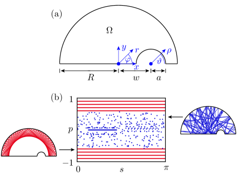
Figure 20: (Color online) (a) Schematic picture of the desymmetrized annular billiard showing the two coordinate systems used in the theoretical derivation of the direct regular-to-chaotic tunneling rates. (b) Poincaré section at the semi-circle boundary (relative tangential momentum $p$ vs arclength $s$) showing regular and chaotic regions for $R=1$, $a=0.15$, and $w=0.45$ with illustrations of trajectories.

In order to determine these direct regular-to-chaotic tunneling rates we proceed similar to the case of the mushroom billiard. We have to evaluate Eq. (13) for the coupling matrix elements $v_{\text{ch},mn}$ and then use Fermi’s golden rule, Eq. (14), to determine the tunneling rates. In the first step the fictitious integrable system $H_{\text{reg}}$ and its eigenstates $\psi_{\text{reg}}^{mn}$ have to be defined. A natural choice for $H_{\text{reg}}$ is the semi-circle billiard which exactly reproduces the whispering-gallery motion in the annular billiard. Its eigenstates are given by

$$\psi_{\text{reg}}^{mn}(r,\varphi)=N_{mn}J_{m}\left(j_{mn}r\right)\sin(m\varphi)$$ (99)

in polar coordinates $(r,\varphi)$, where $J_{m}$ denotes the $m$th Bessel function, $j_{mn}$ is the $n$th root of $J_{m}$, and $N_{mn}=\sqrt{4/\pi}/J_{m-1}(j_{mn})$. The regular states are characterized by the radial quantum number $n=1,2,\dots$ and the azimuthal quantum number $m=1,2,\dots\;$. Hence, the tunneling rates describing the decay of the regular state $\psi_{\text{reg}}^{mn}(r,\varphi)$ will be labeled by $\gamma_{mn}$. Note, that for the annular billiard only those regular states semiclassically exist which localize on tori with angular momentum $p_{mn}=m/j_{mn}>w+a$.

Evaluating Eq. (13) in order to determine the coupling matrix elements $v_{\text{ch},mn}$ between the regular and the chaotic states, an infinite potential difference arises within the small disk of radius $a$ between the Hamiltonian $H$ of the annular and $H_{\text{reg}}$ of the semi-circle billiard, $H-H_{\text{reg}}=\infty$. At the same time for the chaotic states $\psi_{\text{ch}}=0$ holds in that region, which leads to an undefined product “$\infty\cdot 0$”. Similar to the approach presented for the mushroom billiard we circumvent this problem by considering a finite potential difference $W$ for which at the end the limit $W\to\infty$ is performed. In contrast to the mushroom billiard the area of the annular billiard $\Omega$ is included in the area of the semi-circle billiard $\Omega_{\text{reg}}$, $\Omega\subset\Omega_{\text{reg}}$. We find that in this case the derivative of the chaotic states $\psi_{\text{ch}}(\boldsymbol{q})$ enters in Eq. (13). We obtain

$$v_{\text{ch},mn} = a\int\limits_{0}^{\pi}\text{d}\vartheta\,\psi_{\text{reg}}^{mn}(a,\vartheta)\,\partial_{\rho}\psi_{\text{ch}}(\rho=a,\vartheta)$$ (100)

$$= aN_{mn}\int\limits_{0}^{\pi}\text{d}\vartheta\,J_{m}(j_{mn}r)\sin(m\varphi)\partial_{\rho}\psi_{\text{ch}}(a,\vartheta),\quad\;\;\;$$ (101)

where we introduce polar coordinates $(\rho,\vartheta)$ such that $x=\rho\cos(\vartheta)+w$ and $y=\rho\sin(\vartheta)$. Only the integration over $\vartheta$ from $\vartheta=0$ to $\vartheta=\pi$ along the small semi-circle of radius $\rho=a$ remains. Note, that the regular eigenfunctions are given in polar coordinates $(r(\rho,\vartheta),\varphi(\rho,\vartheta))$, while we integrate along $\rho=a$, see Fig. 20(a). Along this half-circle the regular wave function is largest near the point $(\rho,\vartheta)=(a,0)$ for $w>0$. Hence, a random wave description for the chaotic states $\psi_{\text{ch}}(\rho,\vartheta)$ has to respect the Dirichlet boundary conditions on the line $y=0$ and on the small semi-circle of radius $a$.

Such a random wave model can be constructed using the solutions of the annular concentric billiard (Som1978, , §25) as base functions in polar coordinates $(\rho,\vartheta)$

$$\psi_{\text{ch}}(\rho,\vartheta) = \frac{2}{\sqrt{\mathcal{A}_{\text{ch}}}}\sum_{s=1}^{\infty}c_{s}\sin(s\vartheta)$$ (102)

$$\cdot\frac{J_{s}(k\rho)Y_{s}(ka)-J_{s}(ka)Y_{s}(k\rho)}{\sqrt{J_{s}(ka)^{2}+Y_{s}(ka)^{2}}},$$

in which the $c_{s}$ are Gaussian random variables with $\langle c_{s}\rangle=0$ and $\langle c_{s}c_{t}\rangle=\delta_{st}$. Furthermore, $Y_{s}$ denotes the $s$th Bessel function of the second kind. The normalization constant $2$ has been obtained numerically, such that $\langle|\psi_{\text{ch}}|^{2}\rangle=1/\mathcal{A}_{\text{ch}}$ holds far away from the boundary. The chaotic states defined by Eq. (102) fulfill the Schrödinger equation at arbitrary energy $E=k^{2}$. Similar to the mushroom billiard we do not require that the chaotic states decay into the regular island, as Eq. (101) is an integral along a line of the billiard which is not hit by any regular whispering-gallery trajectory. Near the horizontal boundary and away from the small circle $\langle|\psi_{\text{ch}}|^{2}\rangle$ recovers the behavior $1-J_{0}(2k|\rho-a|)$ BaeSchSti1998 ; Ber2002 . Using the radial derivative of $\psi_{\text{ch}}(\rho,\vartheta)$ at $\rho=a$ one finds

$$\partial_{\rho}\psi_{\text{ch}}(\rho=a,\vartheta)=\frac{2k}{\sqrt{\mathcal{A}_{\text{ch}}}}\sum_{s=1}^{\infty}c_{s}\sin(s\vartheta)R_{s}(ka),$$ (103)

in which we use $J_{s+1}(ka)Y_{s}(ka)-J_{s}(ka)Y_{s+1}(ka)=2/(\pi ka)$ (AbrSte1970, , Eq. 9.1.16) and introduce

$$R_{s}(ka):=\frac{2}{\pi ka\sqrt{J_{s}(ka)^{2}+Y_{s}(ka)^{2}}}.$$ (104)

With this result we calculate the tunneling rates at energy $E_{mn}=j_{mn}^{2}$

$$\gamma_{mn} = 2N_{mn}^{2}a^{2}j_{mn}^{2}\sum_{s=1}^{\infty}R_{s}(j_{mn}a)^{2}$$ (105)

$$\cdot\left[\int\limits_{0}^{\pi}\text{d}\vartheta\sin(s\vartheta)J_{m}(j_{mn}r(\vartheta))\sin(m\varphi(\vartheta))\right]^{2}.\quad\;$$

This is our final result predicting the decay of a regular state $\psi_{\text{reg}}^{mn}$ located in the regular whispering-gallery region to the chaotic sea. In Eq. (105), in contrast to the result for the mushroom billiard, Eq. (93), the term $s=1$ is typically not the most important contribution. Here the dominant $s$ increases with energy. In contrast to the prediction of Refs. DorFri1995 ; FriDor1998 no fitting is required.

The numerical determination of tunneling rates using avoided crossings is more difficult for the annular billiard than in the case of the mushroom billiard: In order to affect the chaotic but not the regular component of phase space under parameter variation we increase the radius $a$ of the small inner circle and move its center position $w$ such that its rightmost edge at $w+a$ is constant. We increase $a$ starting from $a=0.05$ until $30$ avoided crossings have occurred or $a=0.4$ is reached. This procedure drastically affects the chaotic states while the regular whispering-gallery modes remain almost unchanged. Note, that under this parameter variation the phase-space structure in the chaotic region changes from macroscopically chaotic to a situation in which additional regular islands and partial barriers appear. With increasing $k$, however, a smaller parameter variation is required and these problems become less relevant.

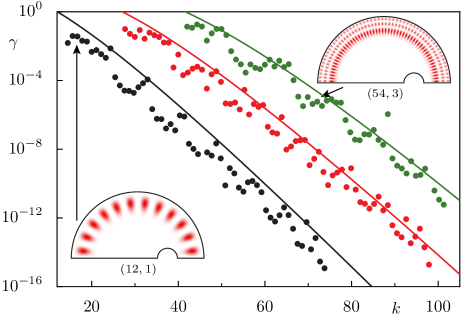
Figure 21: (Color online) Tunneling rates from regular states with quantum numbers $n\leq 3$ vs $k$ for $w+a=0.6$ comparing the prediction of Eq. (105) (solid lines) and numerical rates (dots). The insets show the regular eigenfunctions $\psi_{\text{reg}}^{12,1}$ and $\psi_{\text{reg}}^{54,3}$.

Figure 21 shows the numerical tunneling rates for $w+a=0.6$ and the analytical prediction, Eq. (105), for $a=0.15$ and $w=0.45$. Variations of $a$ with constant $w+a$, as necessary for the numerical rates, affect the prediction by at most a factor of two (not shown). The comparison in Fig. 21 gives qualitative agreement. While some tunneling rates agree with the prediction, deviations of a factor of $100$ appear for other rates.

We believe that these deviations are artifacts of our numerical procedure to determine tunneling rates from avoided crossings Loe2010 . They occur most likely due to beach states which exist in the chaotic region of phase space and look similar to regular states though no quantizing tori can be associated with them DorFri1995 ; FriDor1998 . Numerically we need to analyze avoided crossings between the regular mode and all modes outside the regular island under variation of the shape of the billiard. However, as beach states almost behave like regular states, their energy only slightly varies if the boundary of the billiard is changed. Hence, they rarely show avoided crossings with the regular state. In addition the chaotic states concentrate further away from the regular island and thus give rise to considerably smaller avoided crossings. This leads to artificially reduced numerical tunneling rates. It would be desirable to determine numerical tunneling rates for the annular billiard by other means, e.g., by opening the billiard, to obtain a more quantitative verification of the prediction Eq. (105).

V.3 Disordered wire in a magnetic field

We study two-dimensional nanowires GarGovWoe2002 ; FeiBaeKetRotHucBur2006 ; FeiBaeKetBurRot2009 with one-sided disorder, see Fig. 22(a), in the presence of a homogeneous magnetic field $B$ perpendicular to the wire. Such nanowires have a mixed phase space, see Fig. 22(b). Orbits which only hit the lower flat boundary are regular skipping orbits while those which are reflected at the upper disordered boundary numerically show chaotic motion. The phase space of the wire has a sharp transition from regular to chaotic dynamics. There are no resonance chains inside the regular island and there is no relevant hierarchical region.

In Refs. FeiBaeKetRotHucBur2006 ; FeiBaeKetBurRot2009 it was shown that in such wires the localization lengths $\xi$ increase exponentially with increasing Fermi wave number $k_{F}$ of the electrons. This can be explained by the mixed phase-space structure giving rise to dynamical tunneling between the regular island and the chaotic sea. The dynamical tunneling rates $\gamma$ are directly related to the localization lengths, $\xi\propto 1/\gamma$. We apply the fictitious integrable system approach to determine localization lengths $\xi$ and compare the results to the analytical prediction derived in Refs. FeiBaeKetRotHucBur2006 ; FeiBaeKetBurRot2009 .

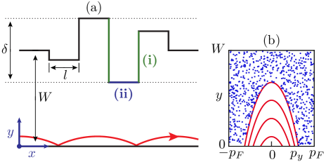
Figure 22: (Color online) (a) Schematic picture of a magnetic wire with one-sided disorder to which leads of width $W$ are attached. The wire is composed of rectangular elements of length $l$ and a uniformly distributed height in $[W-\delta/2,W+\delta/2]$. For the tunneling process contributions (i) along the vertical and (ii) along the horizontal parts of the upper boundary are relevant. (b) A Poincaré section $(y,p_{y})$ at fixed $x$ shows a large regular island (red lines) and the chaotic sea (blue dots).

The nanowire with a disordered boundary is assembled from $L$ rectangular elements to which two leads of width $W$ are attached. The $n$th element has a length $l=W/5$ and a height $h_{n}$ which is uniformly distributed in the interval $[W-\delta/2,W+\delta/2]$ with $\delta=2W/3$. The heights $h_{n}$ are allowed to take $M=20$ different values including the boundaries of the interval. For increasing values of the Fermi wave number $k_{F}$ the magnetic field $B$ is adjusted such that the cyclotron radius $r_{c}=\hbar k_{F}/(eB)$ remains constant, using $r_{c}=3W$. This leaves the classical dynamics unchanged and the semiclassical limit is given by $k_{F}\to\infty$.

In order to apply the fictitious integrable system approach we have to consider a closed billiard. It is obtained by imposing periodic boundary conditions at the positions where the leads are attached. The tunneling rate is given by Fermi’s golden rule, Eq. (14), using the coupling-matrix elements between regular and chaotic states, Eq. (13). Similar to the examples discussed previously we have to find a fictitious integrable system $H_{\text{reg}}$ which resembles the regular part of the phase space and extends it beyond. A reasonable choice is a billiard of length $Ll$ with periodic boundary conditions at $x=0$ and with a boundary at $y=0$ but open for $y>0$. In a magnetic field it shows exactly the same regular phase space as the wire with one disordered boundary and is completely integrable. Its eigenfunctions $\psi_{\text{reg}}^{m}(x,y)$ are given by Bal1999

$$\psi_{\text{reg}}^{m}(x,y)=\frac{1}{\sqrt{lL}}\text{e}^{\text{i}k_{m}x}Z_{m}(y),$$ (106)

where $Z_{m}(y)$ solves a one-dimensional Schrödinger equation with an effective potential due to the magnetic field and $m\geq 1$ is the quantum number in transversal direction. Using this regular system and its eigenstates in Eq. (13) gives

$$v_{\text{ch},m}=\int\limits_{\mathcal{C}}\text{d}s\,\partial_{N}\psi_{\text{ch}}(x(s),y(s))\,\psi_{\text{reg}}^{m}(x(s),y(s)).$$ (107)

As for the annular billiard the derivative of the chaotic states $\partial_{N}\psi_{\text{ch}}(x(s),y(s))$ is in the normal direction along the disordered boundary $\mathcal{C}$, which is parameterized by $s$.

The most important contributions of the integral in Eq. (107) are from rectangular elements of the wire which have the smallest height, i.e. $h_{n}=W-\delta/2$. This follows from the exponential decay of the regular wave functions $\psi_{\text{reg}}^{m}$ in $y$-direction. There are $L/M$ such rectangular elements. The upper boundary of the wire near such an element is composed of (i) two vertical parts ($x=nl$, $y\in[h_{n-1},W-\delta/2]$ and $x=(n+1)l$, $y\in[W-\delta/2,h_{n+1}]$) and (ii) one horizontal part ($x\in[nl,(n+1)l]$, $y=W-\delta/2$).

(i) Let us first consider one vertical contribution to the coupling-matrix elements $v_{\text{ch},m}$ for the fixed $x$-coordinate $x^{*}=nl$. For the chaotic states $\psi_{\text{ch}}$ we employ a random wave model with wave length $k_{F}$ such that the Dirichlet boundary condition at $x=x^{*}$ is fulfilled

$$\psi_{\text{ch}}(r,\varphi)=\frac{2}{\sqrt{\mathcal{A}_{\text{ch}}}}\sum_{s=1}^{\infty}c_{s}J_{s}(k_{F}r)\sin\left(s\varphi-\frac{\pi}{2}s\right),$$ (108)

where the polar coordinates $(r,\varphi)$ are defined by $x=x^{*}+r\cos\varphi$ and $y=W-\delta/2+r\sin\varphi$. The coefficients $c_{s}$ are Gaussian random variables with mean zero and $\langle c_{s}c_{t}\rangle=\delta_{st}$. It will turn out that the form of Eq. (108) is more convenient for the following evaluation than a plane wave ansatz. The derivative of $\psi_{\text{ch}}$ with respect to $x$ at $x=x^{*}$ gives

$$\partial_{x}\psi_{\text{ch}}(x=x^{*},\hat{y})=\frac{2}{\sqrt{\mathcal{A}_{\text{ch}}}}\sum_{s=1}^{\infty}c_{s}\frac{J_{s}(k_{F}\hat{y})s}{\hat{y}},$$ (109)

where $\hat{y}=y-(W-\delta/2)$. Hence, the contribution of one vertical part of the boundary to the coupling-matrix element is (up to a phase $\text{e}^{\text{i}k_{m}x^{*}}$)

$$v_{\text{ch},m}=\frac{2}{\sqrt{\mathcal{A}_{\text{ch}}}}\frac{1}{\sqrt{Ll}}\sum_{s=1}^{\infty}c_{s}\int\limits_{0}^{\infty}\frac{J_{s}(k_{F}\hat{y})s}{\hat{y}}Z_{m}(\hat{y})\,\text{d}\hat{y}.\quad$$ (110)

Here we have replaced the upper integration limit by $\infty$ as $Z_{m}(\hat{y})$ decays exponentially. The sum of $2L/M$ such coupling matrix elements gives according to Fermi’s golden rule, Eq. (14), the direct regular-to-chaotic tunneling contribution of the vertical boundaries

$$\gamma_{m}^{\text{(i)}}=\frac{4}{Ml}\sum_{s=1}^{\infty}s^{2}\left(\int\limits_{0}^{\infty}\frac{J_{s}(k_{F}\hat{y})}{\hat{y}}Z_{m}(\hat{y})\,\text{d}\hat{y}\right)^{2},$$ (111)

where we assume independent coefficients $c_{s}$ for each vertical boundary.

(ii) For the horizontal boundaries we consider the regular wave functions $\psi_{\text{reg}}^{m}(\hat{x},\hat{y}=0)=Z_{m}^{0}\text{e}^{\text{i}k_{m}(nl+\hat{x})}$, where $\hat{x}=x-nl$ and $Z_{m}^{0}=Z_{m}(\hat{y}=0)$. For the chaotic wave function a random wave model respecting the Dirichlet boundary at $\hat{y}=0$ is used,

$$\psi_{\text{ch}}(\hat{x},\hat{y})=\sqrt{\frac{2}{N\mathcal{A}_{\text{ch}}}}\sum_{s=1}^{N}c_{s}\text{e}^{\text{i}(k_{F}\hat{x}\cos\vartheta_{s}+\varphi_{s})}\sin(k_{F}\hat{y}\sin\vartheta_{s}),$$ (112)

where the coefficients $c_{s}$ are Gaussian random variables with mean zero as well as $\langle c_{s}c_{t}\rangle=\delta_{st}$ and the angles $\vartheta_{s}$ and $\varphi_{s}$ are uniformly distributed in $[0,2\pi)$. The derivative of $\psi_{\text{ch}}$ with respect to $\hat{y}$ at $\hat{y}=0$ reads

$$\partial_{\hat{y}}\psi_{\text{ch}}(\hat{x},\hat{y}=0)=\frac{\sqrt{2}k_{F}}{\sqrt{N\mathcal{A}_{\text{ch}}}}\sum_{s=1}^{N}c_{s}\sin\vartheta_{s}\,\text{e}^{\text{i}(k_{F}\hat{x}\cos\vartheta_{s}+\varphi_{s})}.$$ (113)

Hence, we obtain for the contribution of one horizontal part of the boundary to the coupling-matrix element (up to a phase $\text{e}^{\text{i}k_{m}nl}$)

$$v_{\text{ch},m}=\frac{\sqrt{2}k_{F}Z_{m}^{0}}{\sqrt{\mathcal{A}_{\text{ch}}NLl}}\sum_{s}c_{s}\sin\vartheta_{s}\,\text{e}^{\text{i}\varphi_{s}}\int\limits_{0}^{l}\text{d}\hat{x}\,\text{e}^{\text{i}(k_{F}\cos\vartheta_{s}+k_{m})\hat{x}}.$$ (114)

The sum of $L/M$ such coupling matrix elements gives according to Fermi’s golden rule, Eq. (14), the direct regular-to-chaotic tunneling contribution of the horizontal boundaries

$$\gamma_{m}^{\text{(ii)}}=\frac{|Z_{m}^{0}|^{2}}{2\pi Ml}\int\limits_{0}^{2\pi}\text{d}\vartheta\sin^{2}\vartheta\,\frac{2-2\cos\left(lk_{F}\left[\cos\vartheta+\frac{k_{m}}{k_{F}}\right]\right)}{\left(\cos\vartheta+\frac{k_{m}}{k_{F}}\right)^{2}},$$ (115)

where we assume independent coefficients $c_{s}$ for each horizontal boundary. The total tunneling rate is given as the sum of the two contributions, Eq. (111) from the vertical parts of the boundary and Eq. (115) from the horizontal parts of the boundary,

$$\gamma_{m}=\gamma_{m}^{\text{(i)}}+\gamma_{m}^{\text{(ii)}}.$$ (116)

Here we use the approximation that random wave models for the horizontal and vertical boundaries are independent.

We now compare this result for the dynamical tunneling rates $\gamma_{m}$ to the semiclassical prediction of localization lengths $\xi_{m}$ for the wire with one-sided disorder derived in Ref. FeiBaeKetBurRot2009 . For the connection between tunneling rates and localization lengths we use their inverse proportionality HufKetOttSch2002 ; IomFisZas2002 . One finds

$$\gamma_{m}=\frac{v_{x,m}}{\xi_{m}l}=\frac{2k_{m}}{\xi_{m}l},$$ (117)

where $v_{x,m}$ is the velocity of the $m$th mode in $x$-direction and the localization length $\xi_{m}$ is measured in units of the length $l$ of the rectangular elements. Figure 23 compares the localization lengths obtained by the fictitious integrable system approach using Eqs. (116) and (117) with numerically determined $Z_{m}(y)$ (solid lines) to the analytical prediction of Ref. FeiBaeKetBurRot2009 (dashed lines) showing good agreement with deviations smaller than a factor of two.

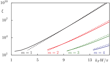
Figure 23: (Color online) Localization lengths of transversal modes in a magnetic wire with one-sided disorder for the mode numbers $m\leq 4$ vs $k_{F}W/\pi$ for $l/W=1/5$ and $\delta=2W/3$. We compare the prediction of Eqs. (116) and (117) (solid lines) and the analytical result of Ref. FeiBaeKetBurRot2009 (dashed lines).

Note, that while in Ref. FeiBaeKetBurRot2009 the localization length is $l$-independent we find for our horizontal contribution an $l$-dependence due to the integral in Eq. (114). This becomes relevant for $l\gg W$ and can be corrected by either changing the upper limit of integration in Eq. (114) from $l$ to $1/k_{F}$ or by choosing an improved $H_{\text{reg}}$. This accounts for the fact that far away from the corners of the disordered boundary there is no tunneling.

V.4 Optical microcavities

Optical microcavities in which photons can be confined in three spatial dimensions are a subject of intensive research as they are relevant for applications such as ultralow-threshold lasers. Especially whispering-gallery cavities such as microdisks, microspheres, and microtoroids have been investigated as they can trap photons for a long time near the boundary by total internal reflection at the optically thinner medium. The corresponding whispering-gallery modes have a very high quality factor $Q$. While the microdisk emits the photons isotropically, cavities with deformed surfaces may additionally lead to directed emission NoeSto1997 ; WieHen2006 ; WieHen2008 ; YanWanDieHenWieYuPflBelYamKan2009 .

The quality factors $Q$ of optical microcavities can be connected to dynamical tunneling rates $\gamma$. These rates can be determined using the fictitious integrable system approach BaeKetLoeWieHen2009 , which will be summarized in this section. For a mode in an open cavity the quality factor $Q$ is related to the corresponding resonance with complex wave number $k=\text{Re}(k)+\text{i}\,\text{Im}(k)$ via

$$Q=-\frac{\text{Re}(k)}{2\text{Im}(k)}.$$ (118)

For cavities with a mixed phase space the quality factor $Q$ of a regular mode has two contributions

$$\frac{1}{Q}=\frac{1}{Q_{\text{1d}}}+\frac{1}{Q_{\text{dyn}}}.$$ (119)

Here $Q_{\text{1d}}$ accounts for the coupling of the regular mode to the continuum. In the case of the circular microcavity Noe1997 it is described by a quasi one-dimensional barrier-tunneling process through an angular momentum barrier. It can be predicted by means of WKB theory or using the numerically determined decay rates of the modes in the circular cavity. Note, that for this contribution the mixed phase-space structure is irrelevant. The second contribution, $Q_{\text{dyn}}$, is given by dynamical tunneling from the regular mode to the chaotic sea, which is strongly coupled to the continuum. Here we assume that there are no further phase-space structures within the chaotic sea that affect the quality factor. A priori it is not obvious, which of the two contributions will dominate.

In order to determine $Q_{\text{dyn}}$ the fictitious integrable system approach can be employed in analogy to hard-wall billiards. It is extended to open cavities in the following way: (i) As a fictitious integrable system $H_{\text{reg}}$ one chooses a cavity such that it resembles the regular dynamics of $H$. The quantum system has resonance states $\psi_{\text{reg}}$. (ii) As a model for the chaotic resonances $\psi_{\text{ch}}$ a random wave model is used, which in addition fulfills the relevant cavity boundary conditions. (iii) The tunneling rate $\gamma$ determines the quality factor $Q_{\text{dyn}}$ by

$$Q_{\text{dyn}}=\frac{2\text{Re}(k)^{2}n_{\Omega}^{2}}{\gamma},$$ (120)

where $n_{\Omega}$ is the refractive index of the cavity. Here it is used that the imaginary part of the wave number is connected to the decay rate of the resonant state via $\gamma=-4n_{\Omega}^{2}\text{Re}(k)\text{Im}(k)$ and Eq. (118).

This approach was developed and applied to the annular microcavity, a microdisk with an air hole, in Ref. BaeKetLoeWieHen2009 . It has a particularly interesting geometry which allows for unidirectional emission and high quality factors simultaneously. An analytical expression for the quality factor $Q_{\text{dyn}}$ was derived which is in very good agreement with the full numerical simulations of Maxwell’s equations.

VI Summary and outlook

We study the direct regular-to-chaotic tunneling process in systems with a mixed phase space. It is dominant in the regime, $h_{\text{eff}}\lesssim A_{\text{reg}}$, where fine-scale structures of the phase space such as nonlinear resonances are not resolved by quantum mechanics. To describe this tunneling process we introduce the fictitious integrable system approach. It uses a decomposition of the Hilbert space into two parts which account for the regular and the chaotic dynamics. This leads to a formula which predicts the direct tunneling rate $\gamma_{m}$ of the $m$th regular state $|\psi_{\text{reg}}^{m}\rangle$ to the chaotic sea, Eq. (7). The fictitious integrable system has to be chosen such that its dynamics resembles the regular dynamics of the original mixed system as closely as possible and extends it beyond its regular region. The determination of the fictitious integrable system is the most difficult step in the application of this approach. For maps the Lie transformation or methods based on the frequency map analysis can be used. A general procedure for billiards is under development.

In Sec. IV dynamical tunneling rates are determined numerically and compared to the prediction of the fictitious integrable system approach for different quantum maps. We find excellent agreement over several orders of magnitude in $\gamma$. For a harmonic oscillator-like island embedded in a chaotic sea it is possible to derive a semiclassical expression for the tunneling rates which depends on the area of the regular region and the effective Planck constant only. Furthermore, in Sec. V we apply the approach to billiard systems, where we use random wave models to describe the chaotic states. For the mushroom billiard the prediction is in excellent agreement with numerical and experimental data. Finally, we apply the approach for direct regular-to-chaotic tunneling rates to the annular billiard, nanowires with one-sided disorder in a magnetic field, and to the quality factors of optical microcavities.

In the semiclassical regime, $h_{\text{eff}}\ll A_{\text{reg}}$, nonlinear resonances lead to enhanced tunneling rates due to resonance-assisted tunneling. This resonance-assisted tunneling mechanism is combined to direct regular-to-chaotic tunneling in Ref. LoeBaeKetSch2010 , leading to a prediction of tunneling rates which is valid from the quantum to the semiclassical regime. For this prediction the direct tunneling rates discussed in this paper, which can be determined using the fictitious integrable system approach, are essential.

Ultimately, it is the aim to obtain a complete semiclassical treatment of the approach also for systems with a generic regular island. This theory should predict tunneling rates and their dependence on the effective Planck constant $h_{\text{eff}}$ directly from classical properties of the regular island, such as its size, shape, and winding number and properties of the chaotic sea, such as unstable fixed points, partial barriers, and transport properties. A promising approach seems to be the complex-path formalism which has been successfully applied to study the tunneling tails of a time-evolved wave packet in mixed regular-chaotic systems ShuIke1995 ; ShuIke1998 ; OniShuIkeTak2001 . Alternatively, a complex time approach Mou2007 ; DenMou2010 can be considered. Using such semiclassical approaches for the prediction of regular-to-chaotic tunneling rates should give further insight into the dynamical tunneling process.

Appendix A Dimensionless Fermi’s golden rule for time-periodic quantum systems

In order to predict dynamical tunneling rates $\gamma_{m}$ we use Fermi’s golden rule for systems with a discrete spectrum. This rate describes the decay $\text{e}^{-\gamma_{m}t}$ of the $m$th regular state to the chaotic sea at most up to the Heisenberg time $\tau_{H}=h_{\text{eff}}/\Delta_{\text{ch}}$. Compared to the standard derivation of Fermi’s golden rule Coh1995 for the continuous case, the incoherent integral over the continuum states is replaced by the incoherent sum over the discrete chaotic states. One finds

$$\Gamma_{m}=\frac{2\pi}{\hbar}\langle|V_{\text{ch},m}|^{2}\rangle\rho_{\text{ch}}$$ (121)

with the chaotic density of states $\rho_{\text{ch}}$ and the average of the modulus squared of the coupling matrix elements $V_{\text{ch},m}$ of the Hamiltonian between energetically close-by chaotic states and the $m$th purely regular state.

We now apply Eq. (121) to time-periodic systems with period $\tau$ and quasi-energies in the interval $[0,\hbar\omega]$ with $\omega=2\pi/\tau$ such that $\rho_{\text{ch}}=N_{\text{ch}}/(\hbar\omega)$. We introduce dimensionless quantities $\gamma_{m}=\Gamma_{m}\tau$ and $v_{\text{ch},m}=V_{\text{ch},m}\tau/\hbar$ leading to

$$\gamma_{m}=N_{\text{ch}}\langle|v_{\text{ch},m}|^{2}\rangle=\sum_{\text{ch}}|v_{\text{ch},m}|^{2}.$$ (122)

Here $v_{\text{ch},m}=\langle\psi_{\text{ch}}|U|\psi_{\text{reg}}^{m}\rangle$ is the coupling matrix element of the time evolution operator $U$ over one period and the mean level spacing is $2\pi/N$.

Appendix B Adapted eigenstates of the harmonic oscillator

For the maps $\mathcal{D}$, which for $R=0$ show a tilted and squeezed harmonic oscillator-like regular island, purely regular states $\psi_{\text{reg}}^{m}(q)$ can be constructed by tilting and squeezing the eigenfunctions of the harmonic oscillator accordingly. One finds Sch2006

$$\psi_{\text{reg}}^{m}(q)=\frac{1}{\sqrt{2^{m}m!}}\left(\frac{\text{Re}(\sigma)}{\pi\hbar_{\text{eff}}}\right)^{\frac{1}{4}}H_{m}\left(\sqrt{\frac{\text{Re}(\sigma)}{\hbar_{\text{eff}}}}q\right)\text{e}^{-\frac{\sigma}{\hbar_{\text{eff}}}\frac{q^{2}}{2}}$$ (123)

with the Hermite polynomials $H_{m}$ and the complex squeezing parameter $\sigma$, which can be obtained from the tilting angle $\theta$ of the elliptic island with respect to the momentum axis and the ratio $\omega$ of its half axes with

$$\text{Re}(\sigma) = \frac{1}{\frac{1}{\omega}\cos^{2}(\theta)+\omega\sin^{2}(\theta)},$$ (124)

$$\text{Im}(\sigma) = \text{Re}(\sigma)\left(\frac{1}{\omega}-\omega\right)\sin(\theta)\cos(\theta).$$ (125)

Here $\theta$ and $\omega$ can be determined from the linearized dynamics of the classical map around the fixed point,

$$\theta = \frac{1}{2}\arctan\left(\frac{\mathcal{M}_{22}-\mathcal{M}_{11}}{\mathcal{M}_{12}-\mathcal{M}_{21}}\right),$$ (126)

$$\omega = \sqrt{\frac{|\mathcal{M}_{12}-\mathcal{M}_{21}|-c}{|\mathcal{M}_{12}-\mathcal{M}_{21}|+c}},\quad$$ (127)

where $c=\sqrt{(\mathcal{M}_{12}+\mathcal{M}_{21})^{2}+(\mathcal{M}_{22}-\mathcal{M}_{11})^{2}}$ and

$$\mathcal{M}=\left(\begin{array}[]{cc}\tfrac{\partial q_{n+1}}{\partial q_{n}}&\tfrac{\partial q_{n+1}}{\partial p_{n}}\\ \tfrac{\partial p_{n+1}}{\partial q_{n}}&\tfrac{\partial p_{n+1}}{\partial p_{n}}\end{array}\right).$$ (128)

Appendix C Derivation of $\mathcal{A}_{\text{ch}}$ for the mushroom billiard

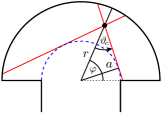
Figure 24: (Color online) All trajectories of the mushroom billiard passing through the point $(r,\varphi)$ with $r>a$ (dot) and angle $|\vartheta|<\vartheta_{c}$ cross the half-circle of radius $a$ (dashed line) and are chaotic. For angles $|\vartheta+\pi|<\vartheta_{c}$ the time-reversed trajectories cross the half-circle and they are chaotic as well.

We want to show how the area $\mathcal{A}_{\text{ch}}$, which is the area of the billiard times the fraction of the chaotic phase-space volume, is determined for the mushroom billiard.

All trajectories which enter the stem of the mushroom or cross the half-circle $r=a$ in the cap are chaotic irrespective of their momentum direction. Additionally the region $r>a$ contains some chaotic dynamics. We denote its contribution to $\mathcal{A}_{\text{ch}}$ by $I$ and obtain for the mushroom billiard

$$\mathcal{A}_{\text{ch}}=2la+\frac{\pi}{2}a^{2}+I.$$ (129)

In order to determine $I$ we consider the fraction $P(r)$ of chaotic trajectories in the cap for $r>a$. It depends on the radial coordinate $r$ only

$$P(r)=\frac{2}{\pi}\arcsin\left(\frac{a}{r}\right),$$ (130)

as can be seen from Fig. 24.

Integrating over the region $r>a$ in the cap of the mushroom gives

$$I = \int\limits_{0}^{\pi}\int\limits_{a}^{R}r\,\text{d}r\,\text{d}\varphi\,P(r)$$ (131)

$$= R^{2}\arcsin\left(\frac{a}{R}\right)+a\sqrt{R^{2}-a^{2}}-\frac{1}{2}\pi a^{2}.$$ (132)

Inserting this expression into Eq. (129) we finally obtain

$$\mathcal{A}_{\text{ch}}=2la+\left[R^{2}\arcsin\left(\frac{a}{R}\right)+a\sqrt{R^{2}-a^{2}}\right]$$ (133)

as the the area of the mushroom billiard times the fraction of the chaotic phase-space volume. For the desymmetrized mushroom used in Sec. V.1 this result has to be divided by two.

References

- (1) L. D. Landau and E. M. Lifshitz, Course of Theoretical Physics, Vol.3: Quantum Mechanics (Pergamon Press, New York, 1991).
- (2) M. J. Davis and E. J. Heller, J. Chem. Phys. 75, 246 (1981).
- (3) I. C. Percival, J. Phys. B 6, L229 (1973).
- (4) M. V. Berry, J. Phys. A 10, 2083 (1977).
- (5) A. Voros, in Stochastic Behavior in Classical and Quantum Hamiltonian Systems (Springer Verlag, Berlin, 1979).
- (6) J. D. Hanson, E. Ott, and T. M. Antonsen, Phys. Rev. A 29, 819 (1984).
- (7) M. Wilkinson, Physica D 21, 341 (1986).
- (8) O. Bohigas, S. Tomsovic, and D. Ullmo, Phys. Rep. 223, 43 (1993).
- (9) S. Tomsovic and D. Ullmo, Phys. Rev. E 50, 145 (1994).
- (10) S. Tomsovic, J. Phys. A 31, 9469 (1998).
- (11) S. C. Creagh, Tunneling in two dimensions, in Tunneling in Complex Systems (World Scientific, Singapore, 1998).
- (12) A. Shudo and K. S. Ikeda, Phys. Rev. Lett. 74, 682 (1995).
- (13) A. Shudo and K. S. Ikeda, Physica D 115, 234 (1998).
- (14) T. Onishi, A. Shudo, K. S. Ikeda, and K. Takahashi, Phys. Rev. E 64, 025201 (2001).
- (15) O. Bohigas, D. Boosé, R. Egydio de Carvalho, and V. Marvulle, Nucl. Phys. A 560, 197 (1993).
- (16) E. Doron and S. D. Frischat, Phys. Rev. Lett. 75, 3661 (1995).
- (17) S. D. Frischat and E. Doron, Phys. Rev. E 57, 1421 (1998).
- (18) O. Brodier, P. Schlagheck, and D. Ullmo, Phys. Rev. Lett. 87, 064101 (2001).
- (19) O. Brodier, P. Schlagheck, and D. Ullmo, Ann. of Phys. 300, 88 (2002).
- (20) C. Eltschka and P. Schlagheck, Phys. Rev. Lett. 94, 014101 (2005).
- (21) P. Schlagheck, C. Eltschka, and D. Ullmo, Resonance- and Chaos-Assisted Tunneling in Progress in Ultrafast Intense Laser Science I, edited by K. Yamanouchi, S. L. Chin, P. Agostini, and G. Ferrante (Springer, Berlin, 2006).
- (22) S. Wimberger, P. Schlagheck, C. Eltschka, and A. Buchleitner, Phys. Rev. Lett. 97, 043001 (2006).
- (23) A. Mouchet, C. Eltschka, and P. Schlagheck, Phys. Rev. E 74, 026211 (2006).
- (24) A. Mouchet, J. Phys. A 40, F663 (2007).
- (25) J. Le Deunff and A. Mouchet, Phys. Rev. E 81, 046205 (2010).
- (26) S. Keshavamurthy, J. Chem. Phys. 122, 114109 (2005).
- (27) S. Keshavamurthy, Phys. Rev. E 72, 045203 (2005).
- (28) V. A. Podolskiy and E. E. Narimanov, Phys. Rev. Lett. 91, 263601 (2003).
- (29) V. A. Podolskiy and E. E. Narimanov, Opt. Lett. 30, 474 (2005).
- (30) M. Sheinman, S. Fishman, I. Guarneri, and L. Rebuzzini, Phys. Rev. A 73, 052110 (2006).
- (31) A. H. Barnett and T. Betcke, Chaos 17, 043125 (2007).
- (32) A. Bäcker, R. Ketzmerick, S. Löck, and L. Schilling, Phys. Rev. Lett. 100, 104101 (2008).
- (33) A. Bäcker, R. Ketzmerick, S. Löck, M. Robnik, G. Vidmar, R. Höhmann, U. Kuhl, and H.-J. Stöckmann, Phys. Rev. Lett. 100, 174103 (2008).
- (34) A. Bäcker, R. Ketzmerick, S. Löck, J. Wiersig, and M. Hentschel, Phys. Rev. A 79, 063804 (2009).
- (35) S. Löck, A. Bäcker, R. Ketzmerick, and P. Schlagheck, Phys. Rev. Lett. 104, 114101 (2010).
- (36) Dynamical Tunneling: Theory and Experiment edited by S. Keshavamurthy and P. Schlagheck (CRC Press, in press).
- (37) D. A. Steck, W. H. Oskay, and M. G. Raizen, Science 293, 274 (2001).
- (38) W. K. Hensinger, H. Häffner, A. Browaeys, N. R. Heckenberg, K. Helmerson, C. McKenzie, G. J. Milburn, W. D. Phillips, S. L. Rolston, H. Rubinsztein-Dunlop, et al., Nature 412, 52 (2001).
- (39) A. Mouchet and D. Delande, Phys. Rev. E 67, 046216 (2003).
- (40) C. Dembowski, H.-D. Gräf, A. Heine, R. Hofferbert, H. Rehfeld, and A. Richter, Phys. Rev. Lett. 84, 867 (2000).
- (41) R. Hofferbert, H. Alt, C. Dembowski, H.-D. Gräf, H. L. Harney, A. Heine, H. Rehfeld, and A. Richter, Phys. Rev. E 71, 046201 (2005).
- (42) T. M. Fromhold, P. B. Wilkinson, R. K. Hayden, L. Eaves, F. W. Sheard, N. Miura, and M. Henini, Phys. Rev. B 65, 155312 (2002).
- (43) H. Schanz, M.-F. Otto, R. Ketzmerick, and T. Dittrich, Phys. Rev. Lett. 87, 070601 (2001).
- (44) A. Bäcker, R. Ketzmerick, and A. G. Monastra, Phys. Rev. Lett. 94, 054102 (2005).
- (45) A. Bäcker, R. Ketzmerick, and A. G. Monastra, Phys. Rev. E 75, 066204 (2007).
- (46) L. Bittrich, Ph.D. thesis, Technische Universität Dresden (2010).
- (47) J. Wiersig and M. Hentschel, Phys. Rev. A 73, 031802(R) (2006).
- (48) S. Shinohara, T. Harayama, T. Fukushima, M. Hentschel, T. Sasaki, and E. E. Narimanov, Phys. Rev. Lett. 104, 163902 (2010).
- (49) J. Yang, S.-B. Lee, S. Moon, S.-Y. Lee, S. W. Kim, T. T. A. Dao, J.-H. Lee, and K. An, Phys. Rev. Lett. 104, 243601 (2010).
- (50) V. A. Podolskiy and E. E. Narimanov, Phys. Lett. A 362, 412 (2007).
- (51) G. Vidmar, H.-J. Stöckmann, M. Robnik, U. Kuhl, R. Höhmann, and S. Grossmann, J. Phys. A 40, 13883 (2007).
- (52) B. Batistić and M. Robnik, J. Phys. A 43, 215101 (2010).
- (53) A. Bäcker, R. Ketzmerick, S. Löck, and N. Mertig, arXiv:1007.4130v1 [nlin.CD] (2010).
- (54) W. A. Lin and L. E. Ballentine, Phys. Rev. Lett. 65, 2927 (1990).
- (55) J. Feist, A. Bäcker, R. Ketzmerick, S. Rotter, B. Huckestein, and J. Burgdörfer, Phys. Rev. Lett. 97, 116804 (2006).
- (56) J. Feist, A. Bäcker, R. Ketzmerick, J. Burgdörfer, and S. Rotter, Phys. Rev. B 80, 245322 (2009).
- (57) M. Sheinman, Master thesis, Technion, Haifa (2005).
- (58) S. Löck, Ph.D. thesis, Technische Universität Dresden (2010).
- (59) M. V. Berry, N. L. Balzas, M. Tabor, and A. Voros, Ann. Phys. 122, 26 (1979).
- (60) F. G. Gustavson, Astron. J. 71, 670 (1966).
- (61) A. Bazzani, M. Giovannozzi, G. Servizi, E. Todesco, and G. Turchetti, Physica D 64, 66 (1993).
- (62) R. Scharf, J. Phys. A 21, 4133 (1988).
- (63) A. J. Lichtenberg and M. A. Lieberman, Regular and Stochastic Motion (Springer, New York, 1983).
- (64) J. Laskar, C. Froeschlé, and A. Celletti, Physica D 56, 253 (1992).
- (65) F. Leyvraz and D. Ullmo, J. Phys. A 29, 2529 (1996).
- (66) F. Borgonovi, I. Guarneri, and D. L. Shepelyansky, Phys. Rev. A 43, 4517 (1991).
- (67) H. Schomerus and J. Tworzydło, Phys. Rev. Lett. 93, 154102 (2004).
- (68) S.-J. Chang and K.-J. Shi, Phys. Rev. A 34, 7 (1986).
- (69) J. P. Keating, F. Mezzadri, and J. M. Robbins, Nonlinearity 12, 579 (1999).
- (70) B. V. Chirikov, Phys. Rep. 52, 263 (1979).
- (71) A. Ishikawa, A. Tanaka, and A. Shudo, J. Phys. A. 40, F397 (2007).
- (72) A. Ishikawa, A. Tanaka, and A. Shudo, Phys. Rev. E 80, 046204 (2009).
- (73) H.-J. Stöckmann and J. Stein, Phys. Rev. Lett. 64, 2215 (1990).
- (74) S. Sridhar, Phys. Rev. Lett. 67, 785 (1991).
- (75) H.-D. Gräf, H. L. Harney, H. Lengeler, C. H. Lewenkopf, C. Rangacharyulu, A. Richter, P. Schardt, and H. A. Weidenmüller, Phys. Rev. Lett. 69, 1296 (1992).
- (76) J. Stein and H.-J. Stöckmann, Phys. Rev. Lett. 68, 2867 (1992).
- (77) H. Alt, A. Bäcker, C. Dembowski, H.-D. Gräf, R. Hofferbert, H. Rehfeld, and A. Richter, Phys. Rev. E 58, 1737 (1998).
- (78) J. Wiersig and M. Hentschel, Phys. Rev. Lett. 100, 033901 (2008).
- (79) L. A. Bunimovich, Chaos 11, 802 (2001).
- (80) E. G. Altmann, A. E. Motter, and H. Kantz, Chaos 15, 033105 (2005).
- (81) H. Tanaka and A. Shudo, Phys. Rev. E 74, 036211 (2006).
- (82) B. Dietz, T. Friedrich, M. Miski-Oglu, A. Richter, and F. Schäfer, Phys. Rev. E 75, 035203 (2007).
- (83) R. S. Lehman, J. Math. Mech. 8, 727 (1959).
- (84) A. Bäcker, R. Schubert, and P. Stifter, Phys. Rev. E 57, 5425 (1998).
- (85) M. V. Berry, J. Phys. A 35, 3025 (2002).
- (86) M. Abramowitz and I. A. Stegun, Handbook of Mathematical Functions (Dover, New York, 1970).
- (87) T. Betcke and L. N. Trefethen, SIAM Rev. 47, 469 (2005).
- (88) A. Sommerfeld, Vorlesungen über theoretische Physik, Band 6: Partielle Differentialgleichungen der Physik (Verlag Harri Deutsch, Thun, 1978).
- (89) A. García-Martín, M. Governale, and P. Wölfle, Phys. Rev. B 66, 233307 (2002).
- (90) L. E. Ballentine, Quantum Mechanics: A Modern Development (World Scientific, Singapore, 1999).
- (91) L. Hufnagel, R. Ketzmerick, M.-F. Otto, and H. Schanz, Phys. Rev. Lett. 89, 154101 (2002).
- (92) A. Iomin, S. Fishman, and G. M. Zaslavsky, Phys. Rev. E 65, 036215 (2002).
- (93) J. U. Nöckel and A. D. Stone, Nature 385, 45 (1997).
- (94) C. Yan, Q. Wang, L. Diehl, M. Hentschel, J. Wiersig, N. Yu, C. Pflüg, M. A. Belkin, M. Yamanishi, H. Kan, et al., Appl. Phys. Lett. 94, 251101 (2009).
- (95) J. U. Nöckel, Ph.D. thesis, Yale University (1997).
- (96) C. Cohen-Tannoudji, Quantum Mechanics Vol. 2 (Wiley, New York, 1995).
- (97) L. Schilling, Ph.D. thesis, Technische Universität Dresden (2006).