Rotating Black String with Nonlinear Source

Abstract

In this paper, we derive rotating black string solutions in the presence of two kinds of nonlinear electromagnetic fields, so called Born-Infeld and power Maxwell invariant. Investigation of the solutions show that for the Born-Infeld black string the singularity is timelike and the asymptotic behavior of the solutions are anti-deSitter, but for power Maxwell invariant solutions, depend on the values of nonlinearity parameter, the singularity may be timelike as well as spacelike and the solutions are not asymptotically anti-deSitter for all values of the nonlinearity parameter. Next, we calculate the conserved quantities of the solutions by using the counterterm method, and find that these quantities do not depend on the nonlinearity parameter. We also compute the entropy, temperature, the angular velocity, the electric charge and the electric potential of the solutions, in which the conserved and thermodynamics quantities satisfy the first law of thermodynamics.

I Introduction

The nonlinear source of general relativity attract the significant attention because of the specific properties such as the black hole solutions with interesting asymptotic behaviors, existence of the soliton solutions, solving the initial singularity in the early universe and so on. The pioneering theory of the nonlinear electrodynamics was proposed, by Born and Infeld BI , with the aim of obtaining a finite value for the self-energy of a pointlike charge. In 1935, Hoffmann Hoff attempted to relate the nonlinear electrodynamics and gravity. He obtained a solution to the Einstein equations for a pointlike Born-Infeld charge, which is devoid of the divergence of the metric at the origin that characterizes the Reissner-Nordström solution.

After these great achievements, because of difficulties that appeared in mathematical formulation, there were not any appreciable attentions to the nonlinear electromagnetic fields. In other word, the Born-Infeld theory was nearly forgotten for several decades, until the interest in nonlinear electrodynamics increased in the context of low energy string theory Frad . The exact solutions of Born-Infeld theory coupled to gravity with or without a cosmological constant have been considered by many authors Demi . The rotating solutions of Born-Infeld gravity with various horizons and investigation of their properties have been considered in Ref. BIpaper .

In recent years there has been aroused interest about black hole solutions whose source is Maxwell invariant raised to the power $s$, i.e., $\left(F_{\mu\nu}F^{\mu\nu}\right)^{s}$ as the source of geometry in Einstein and higher derivative gravity PMIpaper . This theory is considerably richer than that of the linear electromagnetic field and in the special case ($s=1$) it can reduce to linear field. Also, it is valuable to find and analyze the effects of exponent $s$ on the behavior of the new solutions and the laws of black hole mechanics Rasheed . In addition, in higher dimensional gravity, for the special choice $s=d/4$, where $d=$dimension of the spacetime is a multiple of $4$, it yields a traceless Maxwell’s energy-momentum tensor which leads to conformal invariance. The idea is to take advantage of the conformal symmetry to construct the analogues of the four dimensional Reissner-Nordström solutions, in higher dimensions Conformalpaper .

Being motivated by the gravity originated from the nonlinear electromagnetic fields, in this paper we investigate the existence of black string solutions with two types of nonlinear electromagnetic fields, called Born-Infeld theory (BI) and a power of Maxwell invariant (PMI), separately and study their properties. In general, the black string solutions of Einstein gravity have been extensively analyzed in the many literatures. For e.g., charge black string solutions have been studied in Ref. Horne , the nonuniform black strings have been considered in Kudoh , thermodynamics and stability of black strings have been investigated in Gregory ; Dehghani1 and also the properties of the non-abelian and nontrivial topology black string have been studied in Hartmann and Kol , respectively.

Organization of the paper is as follows: we give a brief review of the field equations of Einstein gravity sourced by the nonlinear electromagnetic fields, present charged rotating black string solutions and investigate their properties, especially asymptotic behavior of them. Then, we obtain conserved and thermodynamic quantities of the black string in which satisfy the first law of thermodynamics. We finish our paper with some conclusions.

II Rotating Black String with nonlinear electromagnetic field

The $4$-dimensional action of Einstein gravity with nonlinear electromagnetic field in the presence of cosmological constant is given by

$$I_{G}=-\frac{1}{16\pi}\int_{\mathcal{M}}d^{4}x\sqrt{-g}\left[R-2\Lambda+L(\mathcal{F})\right]-\frac{1}{8\pi}\int_{\partial\mathcal{M}}d^{3}x\sqrt{-\gamma}\Theta(\gamma),$$ (1)

where ${R}$ is the Ricci scalar, $\Lambda$ refers to the negative cosmological constant which in general is equal to $-3/l^{2}$ for asymptotically anti-deSitter solutions, in which $l$ is a scale length factor.

In Eq. (1), $L(\mathcal{F})$ is the Lagrangian of nonlinear electromagnetic field. Here we consider two classes of nonlinear electromagnetic fields, namely Born-Infeld (BI) and power of Maxwell invariant (PMI) in which their Lagrangians are

$$L(\mathcal{F})=\left\{\begin{array}[]{cc}4\beta^{2}\left(1-\sqrt{1+\frac{\mathcal{F}}{2\beta^{2}}}\right)&,\text{BI}\\ -\left(\alpha\mathcal{F}\right)^{s}&,\text{PMI}\end{array}\right..$$ (2)

In this equation, $\beta$ is called the Born-Infeld parameter with dimension of mass, the exponent $s$ is related to the power of nonlinearity, the Maxwell invariant $\mathcal{F}=F_{\mu\nu}F^{\mu\nu}$ in which $F_{\mu\nu}=\partial_{\mu}A_{\nu}-\partial_{\nu}A_{\mu}$ is the electromagnetic field tensor and $A_{\mu}$ is the gauge potential. $L(\mathcal{F})$ reduces to the standard Maxwell form $L(\mathcal{F})=-\mathcal{F}$, when $\beta\rightarrow\infty$ and $s\rightarrow 1$ for BI and PMI theory, respectively.

The last term in Eq. (1) is the Gibbons-Hawking surface term. It is required for the variational principle to be well-defined. The factor $\gamma$ and $\Theta$ are, respectively, the trace of the induced metric and extrinsic curvature for the boundary ${\partial\mathcal{M}}$. Varying the action (1) with respect to the gravitational field $g_{\mu\nu}$ and the gauge field $A_{\mu}$, the field equations are obtained as

$$R_{\mu\nu}-\frac{1}{2}g_{\mu\nu}\left(R-2\Lambda\right)=\alpha T_{\mu\nu},$$ (3)

$$\partial_{\mu}\left(\sqrt{-g}L^{\prime}(\mathcal{F})F^{\mu\nu}\right)=0,$$ (4)

where

$$T_{\mu\nu}=\frac{1}{2}g_{\mu\nu}L(\mathcal{F})-2F_{\mu\lambda}F_{\nu}^{\;\lambda}L^{\prime}(\mathcal{F}),$$ (5)

and $L^{\prime}(\mathcal{F})=\frac{dL(\mathcal{F})}{d\mathcal{F}}$. Our main aim here is to obtain charged rotating black string solutions of the field equations (3) - (5) and investigate their properties. We assume the rotating metric has the following form Lem

$$ds^{2}=-f(r)\left(\Xi dt-ad\phi\right)^{2}+\frac{r^{2}}{l^{4}}\left(adt-\Xi l^{2}d\phi\right)^{2}+\frac{dr^{2}}{f(r)}+\frac{r^{2}}{l^{2}}dz^{2},$$ (6)

where $\Xi=\sqrt{1+a^{2}/l^{2}}$, $a$ is the rotation parameter and the functions $f(r)$ should be determined. The two dimensional space, $t$ =constant and $r$ =constant, has the topology $R\times S^{1}$, and $0\leq\phi<2\pi$, $-\infty<z<\infty$. It is easy to show that for the metric (6), the Kretschmann scalar is

$$R_{\mu\nu\rho\sigma}R^{\mu\nu\rho\sigma}=f^{\prime\prime 2}(r)+\left(\frac{2f^{\prime}(r)}{r}\right)^{2}+\left(\frac{2f(r)}{r^{2}}\right)^{2},$$ (7)

where prime and double primes denote first and second derivative with respect to $r$, respectively. Also one can show that other curvature invariants (such as Ricci scalar, Ricci square, Weyl square and so on) are functions of $f^{\prime\prime}$, $f^{\prime}/r$ and $f/r^{2}$ and therefore it is sufficient to study the Kretschmann scalar for the investigation of the spacetime curvature.

Here, we use the gauge potential ansatz

$$A_{\mu}=h(r)\left(\Xi\delta_{\mu}^{0}-a\delta_{\mu}^{\phi}\right)$$ (8)

in the nonlinear electromagnetic fields equation (4). We obtain

$$h(r)=\left\{\begin{array}[]{cc}-\frac{q}{r}\ \times{{}_{2}F_{1}\left(\left[\frac{1}{2},\frac{1}{4}\right],\left[\frac{5}{4}\right],-\frac{{q^{2}}}{\beta^{2}r^{4}}\right)}&,\text{BI}\\ \left\{\begin{array}[]{cc}q\ln r,&s=\frac{3}{2}\\ -qr^{\lambda},&s\neq\frac{3}{2}\end{array}\right.&,\text{PMI}\end{array}\right.$$ (9)

where $q$ is an integration constant which is related to the electric charge of black string, ${}_{2}F_{1}([a,b],[c],z)$ is hypergeometric function and $\lambda=(2s-3)/(2s-1)$. It is notable that for $s=0,1/2$, the function $h(r)=Constant$, we do not have electromagnetic field and therefore in the rest of the presented paper we exclude these cases from our discussion.

Figure 1: $F_{tr}$ versus $r$ for $\Xi=1.2$, $q=2$, $\beta=5$ ( for BI theory: Bold line) and $s=1$, $s=1.1$, $s=1.2$, $s=1.3$ and $s=1.4$ ( for PMI theory: from right to left, respectively).

One may note that in the linear limit, $\beta\rightarrow\infty$ for BI branch and also $s=1$ for PMI branch, $A_{\mu}$ of Eq. (8) reduces to the gauge potential of linear Maxwell field Dehghani2 . It is easy to show that the non-vanishing components of the electromagnetic field tensor can be written in the form

$$F_{tr} = -\frac{\Xi q}{r}\times\left\{\begin{array}[]{cc}-\beta r\left(\beta^{2}r^{4}+{q^{2}}\right)^{-1/2}&,\text{BI}\\ \left\{\begin{array}[]{cc}-1,&s=\frac{3}{2}\\ \lambda r^{\lambda},&s\neq\frac{3}{2}\end{array}\right.&,\text{PMI}\end{array}\right.,$$ (14)

$$F_{\phi r} = -\frac{a}{\Xi}F_{tr}.$$ (15)

It is remarkable that for $s=3/2$, the electromagnetic field is proportional to $r^{-1}$, in which the same as charged BTZ black hole BTZ ; BTZlike . Also, it is interesting to note that, in general case, the expression of the electric field depends on the nonlinearity parameter ($\beta$ or $s$), and its value coincides with the $4$-dimensional Reissner-Nordström solutions for the linear limit. We can see from Fig. (1), the electromagnetic field vanishes at large values of $r$, as it should be. But near the origin, in contrast with the finite value of the BI theory, the electromagnetic field diverges for PMI theory. In addition, this figure shows that the nonlinearity parameter, $s$, affects on the strength of divergency for $r\rightarrow 0$.

Now, we should fix the sign of the constant $\alpha$ in order to ensure the real solutions. It is easy to show that

$$\mathcal{F}=F_{\mu\nu}F^{\mu\nu}=-2\left[h^{\prime}(r)\right]^{2},$$

and so the power Maxwell invariant, $\left(\alpha\mathcal{F}\right)^{s}$, may be imaginary for positive $\alpha$, when $s$ is fractional. Therefore we set $\alpha=-1$, to have real solutions without loss of generality.

To find the metric function $f(r)$, one may use any components of Eq. (3). The simplest equation is the $rr$ component of these equations, which can be written as

$$2rf^{{}^{\prime}}(r)+2\Lambda r^{2}+2f(r)+\Upsilon(r)=0,$$ (16)

where

$$\Upsilon(r)=\left\{\begin{array}[]{cc}4{\beta}\left[\left(\beta^{2}r^{4}+{q^{2}}\right)^{1/2}-\beta r^{2}\right]&,\text{BI}\\ -r^{2}(2s-1)\left[2h^{{}^{\prime}2}(r)\right]^{s}&,\text{PMI}\end{array}\right..$$

The solutions of Eq. (16) can be written as

$$f(r)=-\frac{\Lambda r^{2}}{3}-{\frac{m}{r}+}\left\{\begin{array}[]{cc}\begin{array}[]{c}{\frac{2{\beta}}{3}}\left[\beta r^{2}-\left(\beta^{2}r^{4}+{q^{2}}\right)^{1/2}\right]+\\ {\frac{4q^{2}}{3r^{2}}}\ _{2}F_{1}{\left(\left[\frac{1}{2},\frac{1}{4}\right],\left[\frac{5}{4}\right],-\frac{{q^{2}}}{\beta^{2}r^{4}}\right)}\end{array}&,\text{BI}\\ &\\ \left\{\begin{array}[]{cc}2^{s-1}\left(2s-1\right)\lambda^{2s-1}q^{2s}r^{\lambda-1},&0<s<\frac{1}{2},s<0\\ \frac{-2^{3/2}q^{3}\ln r}{r},&s=\frac{3}{2}\\ -2^{s-1}\left(2s-1\right)\lambda^{2s-1}q^{2s}r^{\lambda-1},&\text{ Otherwise}\end{array}\right.&,\text{PMI}\end{array}\right.,$$ (17)

where $m$ is the integration constant which is related to mass parameter. One can check that the solutions given by Eq. (17) satisfy all the components of the field equations (3). It is notable that for $s=3/2$, the charge term in (17) includes logarithmic term and is different from other cases. This special solution ($s=3/2$), is very close to BTZ solutions (see BTZlike for more details).

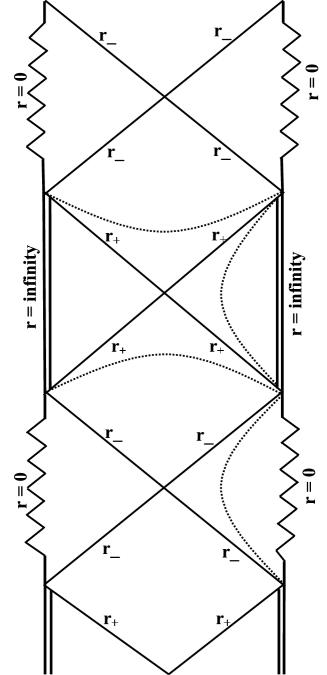
Figure 2: Penrose diagram with negative $\Lambda$ for BI theory with arbitrary $\beta$ and PMI theory when $0<s<\frac{3}{2}$, with two horizons $r_{+}$ and $r_{-}$ and timelike singularity at $r=0$ in which dotted curves represent $r=constant$.

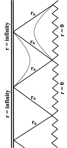
Figure 3: Penrose diagram with negative $\Lambda$ for BI theory with arbitrary $\beta$ and PMI theory when $0<s<\frac{3}{2}$, with one horizon (extreme black string) $r_{+}=r_{-}=r_{h}$ and timelike singularity at $r=0$ in which dotted curves represent $r=constant$.

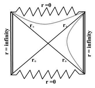
Figure 4: Penrose diagram with negative $\Lambda$ for PMI theory when $s<0$ or $s\geq\frac{3}{2}$, with one horizon $r_{+}$ and spacelike singularity at $r=0$ in which dotted curves represent $r=constant$.

Figure 5: $f(r)$ versus $r$ for $\Lambda=-1$, $q=2$, $m=5$, $\beta=0.7$ for BI theory (Bold line) and $s=1$ (dotted line), $s=2$ (solid line), $s=-2$ (dashed line) for PMI theory.

II.1 Properties of the solutions

The metric function $f(r)$, presented here, differs from the linear $4$ -dimensional Reissner-Nordström black hole solutions; it is notable that the electric charge term in the linear case is proportional to $r^{-2}$, but in the presented metric function, this term depends on the nonlinearity parameter ($\beta$ or $s$). It is notable that in the linear case ($\beta\rightarrow\infty$ for BI or $s=1$ for PMI), the presented solutions reduce to the asymptotically anti-deSitter charged rotating black string Lem .

In order to study the general structure of these spacetime, we first explain the crucial role of negative cosmological constant. One can find that for vanishing cosmological constant, we have physical solutions only for $s=1$ in PMI source and $\beta\rightarrow\infty$ for BI theory (linear source). In other word, for nonlinear sources we need to insert negative cosmological constant in the gravitational field equations to obtain meaningful solutions. This is due to the fact that, repulsive gravitational contribution, arising from nonlinear electromagnetic source, should balance by the attractive contribution of the negative cosmological constant (for more details see CC ).

existence of nonlinear source, the black string solutions exist only in the presence of negative cosmological constant, when the repulsive gravitational contribution, originate from nonlinear electromagnetic source, is balanced by the attraction of the negative cosmological constant.

Second, we investigate the effects of the nonlinear electromagnetic field on the asymptotic behavior of the solutions. The solution of BI theory is asymptotically anti-deSitter for all values of nonlinearity parameter $\beta$. But in PMI solutions the asymptotic behaviors are different. It is worthwhile to mention that for $0<s<\frac{1}{2}$, the asymptotic dominant term of Eq. (17) is third term and the presented solutions are not asymptotically anti-deSitter, but for the cases $s<0$ or $s>\frac{1}{2}$ (include of $s=\frac{3}{2}$), the asymptotic behavior of rotating black string solutions are the same as linear anti-deSitter case Lem . Third, we look for the essential singularity(ies). After some algebraic manipulation, one can show that the Kretschmann scalar (7) with metric function (17) diverges at $r=0$ and is finite for $r\neq 0$. Thus, there is a curvature singularity located at $r=0$. In addition, Penrose diagrams, Figs. (2)-(4) and also Fig. (5) show that the singularity is timelike for BI theory and $0<s<\frac{3}{2}$ in PMI theory, but for $s<0$ or $s\geq\frac{3}{2}$ it is spacelike. Drawing the Penrose diagrams show that the casual structure of the solutions are asymptotically well behaved.

II.2 Conserved quantities

Next, we calculate the conserved quantities of the solutions. To compute the conserved charges of our solutions, we use the approach proposed by Balasubramanian and Kraus in Kraus . This technique was inspired by anti-deSitter/conformal field theory correspondence Mal and consists in adding suitable counterterms $I_{ct}$ to the action of the theory (1) in order to ensure the finiteness of the boundary stress tensor $T_{ab}=\frac{2}{\sqrt{-\gamma}}\frac{\delta I}{\delta\gamma^{ab}}$ derived by the quasilocal energy definition BY . Therefore we supplement the general action (1) with the following boundary counterterm

$$I_{ct}=-\frac{1}{4\pi}\int_{\partial\mathcal{M}}d^{3}x\sqrt{-\gamma}\left(-\frac{1}{l}\right).$$ (18)

Varying the total action ($I_{tot}=I_{G}+I_{ct}$) with respect to the induced metric $\gamma_{ab}$, we find the divergence-free boundary stress-tensor

$$T^{ab}=\frac{\Theta^{ab}-\left(\Theta+\frac{2}{l}\right)\gamma^{ab}}{8\pi},$$ (19)

To compute the conserved charges of the spacetime, one should choose a spacelike surface $\mathcal{B}$ in $\partial\mathcal{M}$ with metric $\sigma_{ij}$, and write the boundary metric in Arnowitt-Deser-Misner form

$$\gamma_{ab}dx^{a}dx^{a}=-N^{2}dt^{2}+\sigma_{ij}\left(d\varphi^{i}+V^{i}dt\right)\left(d\varphi^{j}+V^{j}dt\right),$$

where the coordinates $\varphi^{i}$ are the angular variables parameterizing the hypersurface of constant $r$ around the origin, and $N$ and $V^{i}$ are the lapse and shift functions, respectively. When there is a Killing vector field $\mathcal{\xi}$ on the boundary, the quasilocal conserved quantity associated with the stress tensor of Eq. (19) can be written as

$$Q(\mathcal{\xi)}=\int_{\mathcal{B}}d^{2}x\sqrt{\sigma}T_{ab}n^{a}\mathcal{\ \xi}^{b},$$ (20)

where $\sigma$ is the determinant of the metric $\sigma_{ij}$, $\mathcal{\ \xi}$ and $n^{a}$ are, respectively, the Killing vector field and the unit normal vector on the boundary $\mathcal{B}$. In the context of counterterm method, the limit in which the boundary $\mathcal{B}$ becomes infinite ($\mathcal{B}_{\infty}$) is taken, and the counterterm prescription ensures that the total action and conserved charges are finite Kraus . For boundaries with timelike ($\xi=\partial/\partial t$) and rotational ($\varsigma=\partial/\partial\varphi$) Killing vector fields, one obtains the quasilocal mass and angular momentum

$$M = \int_{\mathcal{B}}d^{2}x\sqrt{\sigma}T_{ab}n^{a}\xi^{b},$$ (21)

$$J = \int_{\mathcal{B}}d^{2}x\sqrt{\sigma}T_{ab}n^{a}\varsigma^{b}.$$ (22)

These quantities are, respectively, the conserved mass and angular momenta of the system enclosed by the boundary $\mathcal{B}$. The mass and angular momentum per unit length of the string when the boundary $\mathcal{B}$ goes to infinity can be calculated through the use of Eqs. (21) and (22). We find

$${M}=\frac{1}{16\pi l}\left(3\Xi^{2}-1\right)m,$$

$${J}=\frac{3}{16\pi l}\Xi ma.$$

For $a=0$ ($\Xi=1$), the angular momentum per unit length vanishes, and therefore $a$ is the rotational parameter of the spacetime.

Next, we obtain the entropy of the black string. Bekenstein argued that the entropy of a black hole is a linear function of the area of its event horizon, which so-called area law Bekenstein and also he proposed a value for the proportionality constant, deduced from a semiclassical calculation of the minimum increase in the area of a black hole when it absorbs a particle. Since the area law of the entropy is universal, and applies to all kinds of black objects in Einstein gravity Bekenstein ; hunt , therefore the entropy per unit length of the black string is

$${S}=\frac{r_{+}^{2}\Xi}{4l}.$$ (23)

Although our solution is not static, the Killing vector

$$\chi=\partial_{t}+\Omega\partial_{\phi},$$ (24)

is the null generator of the event horizon where $\Omega$ is the angular velocity of the outer horizon. By analytic continuation of the metric we can obtain the temperature and angular velocity of the horizon. The analytical continuation of the Lorentzian metric by $t\rightarrow i\tau$ and $a\rightarrow ia$ yields the Euclidean section, whose regularity at $r=r_{+}$ requires that we should identify $\tau\sim\tau+\beta_{+}$ and $\phi\sim\phi+i\Omega\beta_{+}$, where $\beta_{+}$ is the inverse Hawking temperature of the event horizon. We find

$$T_{+}=\beta_{+}^{-1}=\frac{-\Lambda r_{+}}{4\pi\Xi}+\frac{1}{4\pi\Xi}\times\left\{\begin{array}[]{cc}2\beta^{2}r_{+}{\left[1-\left(1+\frac{{q^{2}}}{\beta^{2}r_{+}^{4}}\right)^{1/2}\right]}&,\text{BI}\\ &\\ \left\{\begin{array}[]{cc}\frac{2^{s-1}(2s-1)\lambda^{2s}q^{2s}}{r_{+}^{(2s+1)/(2s-1)}}&0<s<\frac{1}{2}\;,s<0\\ \frac{2^{3/2}q^{3}}{r_{+}^{2}},&s=\frac{3}{2}\\ -\frac{2^{s-1}(2s-1)\lambda^{2s}q^{2s}}{r_{+}^{(2s+1)/(2s-1)}},&\text{ Otherwise}\end{array}\right.&,\text{PMI}\end{array}\right.,$$ (25)

and

$$\Omega=\frac{a}{\Xi l^{2}}.$$ (26)

The next quantity we are going to calculate is the electric charge of the black string. The electric charge per unit length of it, $Q$, can be found by calculating the flux of the electromagnetic field at infinity, yielding

$${Q}=\frac{\Xi}{8\pi}\times\left\{\begin{array}[]{cc}2q&,\text{BI}\\ \left\{\begin{array}[]{cc}2^{3/2}q^{2},&s=\frac{3}{2}\\ -2^{s}\lambda^{2s-1}q^{2s-1},&s\neq\frac{3}{2}\end{array}\right.&,\text{PMI}\end{array}\right.$$ (27)

The electric potential $U$, measured at infinity with respect to the event horizon $r_{+}$, is defined by Cvetic

$$U=A_{\mu}\chi^{\mu}\left|{}_{r\rightarrow\infty}-A_{\mu}\chi^{\mu}\right|_{r=r_{+}},$$ (28)

where $\chi$ is the null generator of the event horizon (24). One can easily obtain the electric potential as

$$U=\frac{q}{\Xi r_{+}}\times\left\{\begin{array}[]{cc}\ {{}_{2}F_{1}\left(\left[\frac{1}{2},\frac{1}{4}\right],\left[\frac{5}{4}\right],-\frac{{q^{2}}}{\beta^{2}r_{+}^{4}}\right)}&,\text{BI}\\ \left\{\begin{array}[]{cc}-r_{+}\ln r_{+},&s=\frac{3}{2}\\ r_{+}^{\lambda+1},&s\neq\frac{3}{2}\end{array}\right.&,\text{PMI}\end{array}\right..$$ (29)

Having the conserved and thermodynamic quantities of the rotating black string at hand, we are in a position to check the first law of black hole thermodynamics. Using the Smarr-type formula for both branches, it is straightforward to calculate the temperature, angular velocity and electric potential in the following manner

$$T=\left(\frac{\partial M}{\partial S}\right)_{J,Q},\text{ \ \ \ \ \ \ }\Omega=\left(\frac{\partial M}{\partial J}\right)_{S,Q},\text{ \ \ \ \ \ \ }U=\left(\frac{\partial M}{\partial Q}\right)_{S,J}$$ (30)

Since the quantities calculated by Eq. (30) coincide with Eqs. (25), (26) and (29), one can conclude that these quantities satisfy the first law of thermodynamics

$$dM=TdS+\Omega d{J}+Ud{Q}.$$ (31)

III Conclusion

In this paper, we obtained a new class of rotating black string solutions in the presence of negative cosmological constant and investigated their properties. The matter fields, in which we considered, are two kinds of nonlinear electromagnetic fields, called Born-Infeld theory and power Maxwell invariant source. As expected, the nonlinearity parameters effected on the electromagnetic field, clearly. Although investigation of nonlinear electromagnetic source is more complicated, but nonlinear sources are more flexible. For e.g., it is interesting that we could obtain the BTZ-like solution for $s=3/2$.

In addition, it is worthwhile to mention that the repulsive gravitational contribution arising from nonlinear sources is balanced by the attractive contribution of the negative cosmological constant. In other words, we did not encounter with physical solutions if we considered the nonlinear sources without $\Lambda$ term.

After presented physical solutions, we investigated their properties. As one can see from Penrose diagrams, the singularity of the Born-Infeld black string is timelike and the asymptotic behavior of the BI solution is anti-deSitter, but for power Maxwell invariant source, the singularity type and the asymptotic behavior of the solutions depend on the values of nonlinearity parameter.

Then by using the counterterm approach, we calculated the conserved quantities of the solutions which they did not change with respect to the linear Maxwell field. Also, using the area law, Gauss law and analytic continuation of the metric, we achieved the entropy, the electric charge and the temperature and angular velocity of the solutions. It is notable that, in contrast with the Born-Infeld black string, the nonlinearity parameter of the power Maxwell invariant solutions effected on the electrical charge. Finally, we obtained the electric potential of the black string and checked that these conserved and thermodynamic quantities satisfy the first law of thermodynamics.