INSTITUT NATIONAL DE RECHERCHE EN INFORMATIQUE ET EN AUTOMATIQUE

Network Flow Algorithms for Structured Sparsity
Julien Mairal — Rodolphe Jenatton — Guillaume Obozinski — Francis Bach N° 7372
 August 2010 

Abstract: We consider a class of learning problems that involve a structured sparsity-inducing norm defined as the sum of $\ell_{\infty}$-norms over groups of variables. Whereas a lot of effort has been put in developing fast optimization methods when the groups are disjoint or embedded in a specific hierarchical structure, we address here the case of general overlapping groups. To this end, we show that the corresponding optimization problem is related to network flow optimization. More precisely, the proximal problem associated with the norm we consider is dual to a quadratic min-cost flow problem. We propose an efficient procedure which computes its solution exactly in polynomial time. Our algorithm scales up to millions of variables, and opens up a whole new range of applications for structured sparse models. We present several experiments on image and video data, demonstrating the applicability and scalability of our approach for various problems.

Key-words: network flow optimization, convex optimization, sparse methods, proximal algorithms

Algorithmes de Flots pour Parcimonie Structurée

Résumé : Nous considérons une classe de problèmes d’apprentissage régularisés par une norme induisant de la parcimonie structurée, définie comme une somme de normes $\ell_{\infty}$ sur des groupes de variables. Alors que de nombreux efforts ont étés mis pour développer des algorithmes d’optimisation rapides lorsque les groupes sont disjoints ou structurés hiérarchiquement, nous nous intéressons au cas général de groupes avec recouvrement. Nous montrons que le problème d’optimisation correspondant est lié à l’optimisation de flots sur un réseau. Plus précisément, l’opérateur proximal associé à la norme que nous considérons est dual à la minimisation d’un coût quadratique de flot sur un graphe particulier. Nous proposons une procédure efficace qui calcule cette solution en un temps polynomial. Notre algorithme peut traiter de larges problèmes, comportant des millions de variables, et ouvre de nouveaux champs d’applications pour les modèles parcimonieux structurés. Nous présentons diverses expériences sur des données d’images et de vidéos, qui démontrent l’utilité et l’efficacité de notre approche pour résoudre de nombreux problèmes.

Mots-clés : optimisation de flots, optimisation convexe, méthodes parcimonieuses, algorithmes proximaux

1 Introduction

Sparse linear models have become a popular framework for dealing with various unsupervised and supervised tasks in machine learning and signal processing. In such models, linear combinations of small sets of variables are selected to describe the data. Regularization by the $\ell_{1}$-norm has emerged as a powerful tool for addressing this combinatorial variable selection problem, relying on both a well-developed theory (see [1] and references therein) and efficient algorithms [2, 3, 4].

The $\ell_{1}$-norm primarily encourages sparse solutions, regardless of the potential structural relationships (e.g., spatial, temporal or hierarchical) existing between the variables. Much effort has recently been devoted to designing sparsity-inducing regularizations capable of encoding higher-order information about allowed patterns of non-zero coefficients [5, 6, 7, 8, 9], with successful applications in bioinformatics [6, 10], topic modeling [11] and computer vision [8].

By considering sums of norms of appropriate subsets, or groups, of variables, these regularizations control the sparsity patterns of the solutions. The underlying optimization problem is usually difficult, in part because it involves nonsmooth components. Proximal methods have proven to be effective in this context, essentially because of their fast convergence rates and their ability to deal with large problems [3, 4]. While the settings where the penalized groups of variables do not overlap [12] or are embedded in a tree-shaped hierarchy [11] have already been studied, sparsity-inducing regularizations of general overlapping groups have, to the best of our knowledge, never been considered within the proximal method framework.

This paper makes the following contributions:

• It shows that the proximal operator associated with the structured norm we consider can be computed by solving a quadratic min-cost flow problem, thereby establishing a connection with the network flow optimization literature.

• It presents a fast and scalable procedure for solving a large class of structured sparse regularized problems, which, to the best of our knowledge, have not been addressed efficiently before.

• It shows that the dual norm of the sparsity-inducing norm we consider can also be evaluated efficiently, which enables us to compute duality gaps for the corresponding optimization problems.

• It demonstrates that our method is relevant for various applications, from video background subtraction to estimation of hierarchical structures for dictionary learning of natural image patches.

2 Structured Sparse Models

We consider in this paper convex optimization problems of the form

$$\min_{{\mathbf{w}}\in{\mathbb{R}}^{p}}f({\mathbf{w}})+\lambda\Omega({\mathbf{w}}),$$ (1)

where $f:{\mathbb{R}}^{p}\to{\mathbb{R}}$ is a convex differentiable function and $\Omega:{\mathbb{R}}^{p}\to{\mathbb{R}}$ is a convex, nonsmooth, sparsity-inducing regularization function. When one knows a priori that the solutions of this learning problem only have a few non-zero coefficients, $\Omega$ is often chosen to be the $\ell_{1}$-norm, leading for instance to the Lasso [13]. When these coefficients are organized in groups, a penalty encoding explicitly this prior knowledge can improve the prediction performance and/or interpretability of the learned models [12, 14, 15, 16]. Such a penalty might for example take the form

$$\Omega({\mathbf{w}})\,\triangleq\,\sum_{g\in{\mathcal{G}}}\eta_{g}\max_{j\in g}|{\mathbf{w}}_{j}|\,=\,\sum_{g\in{\mathcal{G}}}\eta_{g}\|{\mathbf{w}}_{g}\|_{\infty},$$ (2)

where ${\mathcal{G}}$ is a set of groups of indices, ${\mathbf{w}}_{j}$ denotes the $j$-th coordinate of ${\mathbf{w}}$ for $j$ in $[1;p]\triangleq\{1,\ldots,p\}$, the vector ${\mathbf{w}}_{g}$ in $\mathbb{R}^{|g|}$ represents the coefficients of ${\mathbf{w}}$ indexed by $g$ in ${\mathcal{G}}$, and the scalars $\eta_{g}$ are positive weights. A sum of $\ell_{2}$-norms is also used in the literature [7], but the $\ell_{\infty}$-norm is piecewise linear, a property that we take advantage of in this paper. Note that when ${\mathcal{G}}$ is the set of singletons of $[1;p]$, we get back the $\ell_{1}$-norm.

If ${\mathcal{G}}$ is a more general partition of $[1;p]$, variables are selected in groups rather than individually. When the groups overlap, $\Omega$ is still a norm and sets groups of variables to zero together [5]. The latter setting has first been considered for hierarchies [7, 10, 17], and then extended to general group structures [5]. Solving Eq. (1) in this context becomes challenging and is the topic of this paper. Following [11] who tackled the case of hierarchical groups, we propose to approach this problem with proximal methods, which we now introduce.

2.1 Proximal Methods

In a nutshell, proximal methods can be seen as a natural extension of gradient-based techniques, and they are well suited to minimizing the sum $f+\lambda\Omega$ of two convex terms, a smooth function $f$ —continuously differentiable with Lipschitz-continuous gradient— and a potentially non-smooth function $\lambda\Omega$ (see [18] and references therein). At each iteration, the function $f$ is linearized at the current estimate ${\mathbf{w}}_{0}$ and the so-called proximal problem has to be solved:

$$\min_{{\mathbf{w}}\in\mathbb{R}^{p}}f({\mathbf{w}}_{0})+({\mathbf{w}}-{\mathbf{w}}_{0})^{\top}\nabla f({\mathbf{w}}_{0})+\lambda\Omega({\mathbf{w}})+{\displaystyle\frac{L}{2}}\|{\mathbf{w}}-{\mathbf{w}}_{0}\|_{2}^{2}.$$

The quadratic term keeps the solution in a neighborhood where the current linear approximation holds, and $L\!>\!0$ is an upper bound on the Lipschitz constant of $\nabla f$. This problem can be rewritten as

$$\min_{{\mathbf{w}}\in\mathbb{R}^{p}}{\displaystyle\frac{1}{2}}\left\|{\mathbf{u}}-{\mathbf{w}}\right\|_{2}^{2}+\lambda^{\prime}\Omega({\mathbf{w}}),$$ (3)

with $\lambda^{\prime}\triangleq\lambda/L$, and ${\mathbf{u}}\triangleq{\mathbf{w}}_{0}-\frac{1}{L}\nabla f({\mathbf{w}}_{0})$. We call proximal operator associated with the regularization $\lambda^{\prime}\Omega$ the function that maps a vector ${\mathbf{u}}$ in $\mathbb{R}^{p}$ onto the (unique, by strong convexity) solution ${\mathbf{w}}^{\star}$ of Eq. (3). Simple proximal method use ${\mathbf{w}}^{\star}$ as the next iterate, but accelerated variants [3, 4] are also based on the proximal operator and require to solve problem (3) exactly and efficiently to enjoy their fast convergence rates. Note that when $\Omega$ is the $\ell_{1}$-norm, the solution of Eq. (3) is obtained by a soft-thresholding [18].

The approach we develop in the rest of this paper extends [11] to the case of general overlapping groups when $\Omega$ is a weighted sum of $\ell_{\infty}$-norms, broadening the application of these regularizations to a wider spectrum of problems.

3 A Quadratic Min-Cost Flow Formulation

In this section, we show that a convex dual of problem (3) for general overlapping groups $\mathcal{G}$ can be reformulated as a quadratic min-cost flow problem. We propose an efficient algorithm to solve it exactly, as well as a related algorithm to compute the dual norm of $\Omega$. We start by considering the dual formulation to problem (3) introduced in [11], for the case where $\Omega$ is a sum of $\ell_{\infty}$-norms:

Lemma 1 (Dual of the proximal problem [11])

Given ${\mathbf{u}}$ in $\mathbb{R}^{p}$, consider the problem

$$\min_{{\boldsymbol{\xi}}\in\mathbb{R}^{p\times|\mathcal{G}|}}\frac{1}{2}\|{\mathbf{u}}-\sum_{g\in\mathcal{G}}{\boldsymbol{\xi}}^{g}\|^{2}_{2}~{}~{}\mbox{ s.t. }~{}~{}\forall g\in\mathcal{G},\ \|{\boldsymbol{\xi}}^{g}\|_{1}\leq\lambda\eta_{g}~{}~{}~{}\mbox{ and }~{}~{}~{}\,{\boldsymbol{\xi}}^{g}_{j}=0\,\mbox{ if }\,j\notin g,$$ (4)

where ${\boldsymbol{\xi}}\!=\!({\boldsymbol{\xi}}^{g})_{g\in\mathcal{G}}$ is in $\mathbb{R}^{p\times|\mathcal{G}|}$, and ${\boldsymbol{\xi}}^{g}_{j}$ denotes the $j$-th coordinate of the vector ${\boldsymbol{\xi}}^{g}$. Then, every solution ${\boldsymbol{\xi}}^{\star}\!=\!({\boldsymbol{\xi}}^{\star g})_{g\in\mathcal{G}}$ of Eq. (4) satisfies ${\mathbf{w}}^{\star}\!=\!{\mathbf{u}}\!-\!\sum_{g\in\mathcal{G}}{\boldsymbol{\xi}}^{\star g}$, where ${\mathbf{w}}^{\star}$ is the solution of Eq. (3).

Without loss of generality, we assume from now on that the scalars ${\mathbf{u}}_{j}$ are all non-negative, and we constrain the entries of ${\boldsymbol{\xi}}$ to be non-negative. We now introduce a graph modeling of problem (4).

3.1 Graph Model

Let $G$ be a directed graph $G=(V,E,s,t)$, where $V$ is a set of vertices, $E\subseteq V\times V$ a set of arcs, $s$ a source, and $t$ a sink. Let $c$ and $c^{\prime}$ be two functions on the arcs, $c:E\to{\mathbb{R}}$ and $c^{\prime}:E\to{\mathbb{R}}^{+}$, where $c$ is a cost function and $c^{\prime}$ is a non-negative capacity function. A flow is a non-negative function on arcs that satisfies capacity constraints on all arcs (the value of the flow on an arc is less than or equal to the arc capacity) and conservation constraints on all vertices (the sum of incoming flows at a vertex is equal to the sum of outgoing flows) except for the source and the sink.

We introduce a canonical graph $G$ associated with our optimization problem, and uniquely characterized by the following construction:
 (i) $V$ is the union of two sets of vertices $V_{u}$ and $V_{gr}$, where $V_{u}$ contains exactly one vertex for each index $j$ in $[1;p]$, and $V_{gr}$ contains exactly one vertex for each group $g$ in ${\mathcal{G}}$. We thus have $|V|=|{\mathcal{G}}|+p$. For simplicity, we identify groups and indices with the vertices of the graph.
 (ii) For every group $g$ in ${\mathcal{G}}$, $E$ contains an arc $(s,g)$. These arcs have capacity $\lambda\eta_{g}$ and zero cost.
 (iii) For every group $g$ in ${\mathcal{G}}$, and every index $j$ in $g$, $E$ contains an arc $(g,j)$ with zero cost and infinite capacity. We denote by ${\boldsymbol{\xi}}_{j}^{g}$ the flow on this arc.
 (iv) For every index $j$ in $[1;p]$, $E$ contains an arc $(j,t)$ with infinite capacity and a cost $c_{j}\!\triangleq\!\frac{1}{2}({\mathbf{u}}_{j}-{\boldsymbol{\bar{\xi}}}_{j})^{2}$, where ${\boldsymbol{\bar{\xi}}}_{j}$ is the flow on $(j,t)$. Note that by flow conservation, we necessarily have ${\boldsymbol{\bar{\xi}}}_{j}\!=\!\sum_{g\in{\mathcal{G}}}{{\boldsymbol{\xi}}_{j}^{g}}$.

Examples of canonical graphs are given in Figures 1(a)-1(c). The flows ${\boldsymbol{\xi}}_{j}^{g}$ associated with $G$ can now be identified with the variables of problem (4): indeed, the sum of the costs on the edges leading to the sink is equal to the objective function of (4), while the capacities of the arcs $(s,g)$ match the constraints on each group. This shows that finding a flow minimizing the sum of the costs on such a graph is equivalent to solving problem (4).

When some groups are included in others, the canonical graph can be simplified to yield a graph with a smaller number of edges. Specifically, if $h$ and $g$ are groups with $h\subset g$, the edges $(g,j)$ for $j\in h$ carrying a flow ${\boldsymbol{\xi}}^{g}_{j}$ can be removed and replaced by a single edge $(g,h)$ of infinite capacity and zero cost, carrying the flow $\sum_{j\in h}{\boldsymbol{\xi}}^{g}_{j}$. This simplification is illustrated in Figure 1(d), with a graph equivalent to the one of Figure 1(c). This does not change the optimal value of ${\boldsymbol{\bar{\xi}}}^{\star}$, which is the quantity of interest for computing the optimal primal variable ${\mathbf{w}}^{\star}$. We present in Appendix A a formal definition of equivalent graphs. These simplifications are useful in practice, since they reduce the number of edges in the graph and improve the speed of the algorithms we are now going to present.

(a) ${\mathcal{G}}\!=\!\{g\!=\!\{1,2,3\}\}$.

(b) ${\mathcal{G}}\!=\!\{g\!=\!\{1,2\},h\!=\!\{2,3\}\}$.

(c) ${\mathcal{G}}\!=\!\{g\!=\!\{1,2,3\},h\!=\!\{2,3\}\}$.

(d) ${\mathcal{G}}\!=\!\{g\!=\!\{1\}\cup h,h\!=\!\{2,3\}\}$.

Figure 1: Graph representation of simple proximal problems with different group structures ${\mathcal{G}}$. The three indices $1,2,3$ are represented as grey squares, and the groups $g,h$ in ${\mathcal{G}}$ as red discs. The source is linked to every group $g,h$ with respective maximum capacity $\lambda\eta_{g},\lambda\eta_{h}$ and zero cost. Each variable ${\mathbf{u}}_{j}$ is linked to the sink $t$, with an infinite capacity, and with a cost $c_{j}\!\triangleq\!\frac{1}{2}({\mathbf{u}}_{j}-{\boldsymbol{\bar{\xi}}}_{j})^{2}$. All other arcs in the graph have zero cost and infinite capacity. They represent inclusion relations in-between groups, and between groups and variables. The graphs 1(c) and 1(d) correspond to a special case of tree-structured hierarchy in the sense of [11]. Their min-cost flow problems are equivalent.

3.2 Computation of the Proximal Operator

Quadratic min-cost flow problems have been well studied in the operations research literature [19]. One of the simplest cases, where ${\mathcal{G}}$ contains a single group $g$ as in Figure 1(a), can be solved by an orthogonal projection on the $\ell_{1}$-ball of radius $\lambda\eta_{g}$. It has been shown, both in machine learning [20] and operations research [19, 21], that such a projection can be done in $O(p)$ operations. When the group structure is a tree as in Figure 1(d), strategies developed in the two communities are also similar [11, 19], and solve the problem in $O(pd)$ operations, where $d$ is the depth of the tree.

The general case of overlapping groups is more difficult. Hochbaum and Hong have shown in [19] that quadratic min-cost flow problems can be reduced to a specific parametric max-flow problem, for which an efficient algorithm exists [22]. While this approach could be used to solve Eq. (4), it ignores the fact that our graphs have non-zero costs only on edges leading to the sink. To take advantage of this specificity, we propose the dedicated Algorithm 1. Our method clearly shares some similarities with a simplified version of [22] presented in [23], namely a divide and conquer strategy. Nonetheless, we performed an empirical comparison described in Appendix D, which shows that our dedicated algorithm has significantly better performance in practice.

Algorithm 1 Computation of the proximal operator for overlapping groups.

1:  Inputs: ${\mathbf{u}}\in\mathbb{R}^{p}$, a set of groups ${\mathcal{G}}$, positive weights $(\eta_{g})_{g\in{\mathcal{G}}}$, and $\lambda$ (regularization parameter).

2:  Build the initial graph $G_{0}=(V_{0},E_{0},s,t)$ as explained in Section 3.2.

3:  Compute the optimal flow: ${\boldsymbol{\bar{\xi}}}\leftarrow\text{{computeFlow}}(V_{0},E_{0})$.

4:  Return: ${\mathbf{w}}={\mathbf{u}}-{\boldsymbol{\bar{\xi}}}$ (optimal solution of the proximal problem).

Function computeFlow($V=V_{u}\cup V_{gr},E$)

1:  Projection step: ${\boldsymbol{\gamma}}\leftarrow\operatornamewithlimits{arg\,min}_{\boldsymbol{\gamma}}\sum_{j\in V_{u}}\frac{1}{2}({\mathbf{u}}_{j}-{\boldsymbol{\gamma}}_{j})^{2}~{}~{}\text{s.t.}~{}~{}\sum_{j\in V_{u}}{\boldsymbol{\gamma}}_{j}\leq\lambda\sum_{g\in V_{gr}}\eta_{g}.$

2:  For all nodes $j$ in $V_{u}$, set ${\boldsymbol{\gamma}}_{j}$ to be the capacity of the arc $(j,t)$.

3:  Max-flow step: Update $({\boldsymbol{\bar{\xi}}}_{j})_{j\in V_{u}}$ by computing a max-flow on the graph $(V,E,s,t)$.

4:  if  $\exists~{}j\in V_{u}~{}~{}\text{s.t.}~{}~{}{\boldsymbol{\bar{\xi}}}_{j}\neq{\boldsymbol{\gamma}}_{j}$ then

5:     Denote by $(s,V^{+})$ and $(V^{-},t)$ the two disjoint subsets of $(V,s,t)$ separated by the minimum $(s,t)$-cut of the graph, and remove the arcs between $V^{+}$ and $V^{-}$. Call $E^{+}$ and $E^{-}$ the two remaining disjoint subsets of $E$ corresponding to $V^{+}$ and $V^{-}$.

6:     $({\boldsymbol{\bar{\xi}}}_{j})_{j\in V_{u}^{+}}\leftarrow\text{{computeFlow}}(V^{+},E^{+})$.

7:     $({\boldsymbol{\bar{\xi}}}_{j})_{j\in V_{u}^{-}}\leftarrow\text{{computeFlow}}(V^{-},E^{-})$.

8:  end if

9:  Return: $({\boldsymbol{\bar{\xi}}}_{j})_{j\in V_{u}}$.

Informally, computeFlow$(V_{0},E_{0})$ returns the optimal flow vector ${\boldsymbol{\bar{\xi}}}$, proceeding as follows: This function first solves a relaxed version of problem Eq. (4) obtained by replacing the sum of the vectors ${\boldsymbol{\xi}}^{g}$ by a single vector ${\boldsymbol{\gamma}}$ whose $\ell_{1}$-norm should be less than, or equal to, the sum of the constraints on the vectors ${\boldsymbol{\xi}}^{g}$. The optimal vector ${\boldsymbol{\gamma}}$ therefore gives a lower bound $||{\mathbf{u}}-{\boldsymbol{\gamma}}||_{2}^{2}/2$ on the optimal cost. Then, the maximum-flow step [24] tries to find a feasible flow such that the vector ${\boldsymbol{\bar{\xi}}}$ matches ${\boldsymbol{\gamma}}$. If ${\boldsymbol{\bar{\xi}}}={\boldsymbol{\gamma}}$, then the cost of the flow reaches the lower bound, and the flow is optimal. If ${\boldsymbol{\bar{\xi}}}\neq{\boldsymbol{\gamma}}$, the lower bound cannot be reached, and we construct a minimum $(s,t)$-cut of the graph [25] that defines two disjoints sets of nodes $V^{+}$ and $V^{-}$; $V^{+}$ is the part of the graph that can potentially receive more flow from the source, whereas all arcs linking $s$ to $V^{-}$ are saturated. The properties of a min $(s,t)$-cut [26] imply that there are no arcs from $V^{+}$ to $V^{-}$ (arcs inside $V$ have infinite capacity by construction), and that there is no flow on arcs from $V^{-}$ to $V^{+}$. At this point, it is possible to show that the value of the optimal min-cost flow on these arcs is also zero. Thus, removing them yields an equivalent optimization problem, which can be decomposed into two independent problems of smaller size and solved recursively by the calls to computeFlow$(V^{+},E^{+})$ and computeFlow$(V^{-},E^{-})$. Note that when $\Omega$ is the $\ell_{1}$-norm, our algorithm solves problem (4) during the first projection step in line $1$ and stops. A formal proof of correctness of Algorithm 1 and further details are relegated to Appendix B.

The approach of [19, 22] is guaranteed to have the same worst-case complexity as a single max-flow algorithm. However, we have experimentally observed a significant discrepancy between the worst case and empirical complexities for these flow problems, essentially because the empirical cost of each max-flow is significantly smaller than its theoretical cost. Despite the fact that the worst-case guarantee of our algorithm is weaker than their (up to a factor $|V|$), it is more adapted to the structure of our graphs and has proven to be much faster in our experiments (see supplementary material).

Some implementation details are crucial to the efficiency of the algorithm:

• Exploiting maximal connected components: When there exists no arc between two subsets of $V$, it is possible to process them independently to solve the global min-cost flow problem. To that effect, before calling the function computeFlow($V,E$), we look for maximal connected components $(V_{1},E_{1}),\ldots,(V_{N},E_{N})$ and call sequentially the procedure computeFlow($V_{i},E_{i}$) for $i$ in $[1;N]$.

• Efficient max-flow algorithm: We have implemented the “push-relabel” algorithm of [24] to solve our max-flow problems, using classical heuristics that significantly speed it up in practice (see [24, 27]). Our implementation uses the so-called “highest-active vertex selection rule, global and gap heuristics” (see [24, 27]), and has a worst-case complexity of $O(|V|^{2}|E|^{1/2})$ for a graph $(V,E,s,t)$. This algorithm leverages the concept of pre-flow that relaxes the definition of flow and allows vertices to have a positive excess.

• Using flow warm-restarts: Our algorithm can be initialized with any valid pre-flow, enabling warm-restarts when the max-flow is called several times as in our algorithm.

• Improved projection step: The first line of the procedure computeFlow can be replaced by ${\boldsymbol{\gamma}}\leftarrow\operatornamewithlimits{arg\,min}_{\boldsymbol{\gamma}}\sum_{j\in V_{u}}\frac{1}{2}({\mathbf{u}}_{j}-{\boldsymbol{\gamma}}_{j})^{2}~{}~{}\text{s.t.}~{}~{}\sum_{j\in V_{u}}{\boldsymbol{\gamma}}_{j}\leq\lambda\sum_{g\in V_{gr}}\eta_{g}~{}\text{and}~{}|{\boldsymbol{\gamma}}_{j}|\leq\lambda\sum_{g\ni j}\eta_{g}.$ The idea is that the structure of the graph will not allow ${\boldsymbol{\bar{\xi}}}_{j}$ to be greater than $\lambda\sum_{g\ni j}\eta_{g}$ after the max-flow step. Adding these additional constraints leads to better performance when the graph is not well balanced. This modified projection step can still be computed in linear time [21].

3.3 Computation of the Dual Norm

The dual norm $\Omega^{*}$ of $\Omega$, defined for any vector ${\boldsymbol{\kappa}}$ in $\mathbb{R}^{p}$ by $\Omega^{*}({\boldsymbol{\kappa}})\triangleq\max_{\Omega({\mathbf{z}})\leq 1}{\mathbf{z}}^{\top}{\boldsymbol{\kappa}}$, is a key quantity to study sparsity-inducing regularizations [5, 17, 28]. We use it here to monitor the convergence of the proximal method through a duality gap, and define a proper optimality criterion for problem (1). We denote by $f^{*}$ the Fenchel conjugate of $f$ [29], defined by $f^{*}({\boldsymbol{\kappa}})\triangleq\sup_{{\mathbf{z}}}[{\mathbf{z}}^{\top}{\boldsymbol{\kappa}}-f({\mathbf{z}})]$. The duality gap for problem (1) can be derived from standard Fenchel duality arguments [29] and it is equal to $f({\mathbf{w}})+\lambda\Omega({\mathbf{w}})+f^{*}(-{\boldsymbol{\kappa}})\ \text{for}\ {\mathbf{w}},{\boldsymbol{\kappa}}\ \text{in}\ \mathbb{R}^{p}\ \text{with}\ \Omega^{*}({\boldsymbol{\kappa}})\leq\lambda$. Therefore, evaluating the duality gap requires to compute efficiently $\Omega^{*}$ in order to find a feasible dual variable ${\boldsymbol{\kappa}}$. This is equivalent to solving another network flow problem, based on the following variational formulation:

$$\Omega^{*}({\boldsymbol{\kappa}})=\!\!\!\min_{{\boldsymbol{\xi}}\in\mathbb{R}^{p\times|\mathcal{G}|}}\!\!\!\tau\quad\text{s.t.}\quad\sum_{g\in\mathcal{G}}{\boldsymbol{\xi}}^{g}={\boldsymbol{\kappa}},\ \text{and}\ \forall g\in\mathcal{G},\ \|{\boldsymbol{\xi}}^{g}\|_{1}\leq\tau\eta_{g}~{}~{}\text{with}~{}~{}\ {\boldsymbol{\xi}}_{j}^{g}=0\ \text{if}\ j\notin g.$$ (5)

In the network problem associated with (12), the capacities on the arcs $(s,g)$, $g\in{\mathcal{G}}$, are set to $\tau\eta_{g}$, and the capacities on the arcs $(j,t)$, $j$ in $[1;p]$, are fixed to ${\boldsymbol{\kappa}}_{j}$. Solving problem (12) amounts to finding the smallest value of $\tau$, such that there exists a flow saturating the capacities ${\boldsymbol{\kappa}}_{j}$ on the arcs leading to the sink $t$ (i.e., ${\boldsymbol{\bar{\xi}}}={\boldsymbol{\kappa}}$). Equration (12) and the algorithm below are proven to be correct in Appendix B.

Algorithm 2 Computation of the dual norm.

1:  Inputs: ${\boldsymbol{\kappa}}\in\mathbb{R}^{p}$, a set of groups ${\mathcal{G}}$, positive weights $(\eta_{g})_{g\in{\mathcal{G}}}$.

2:  Build the initial graph $G_{0}=(V_{0},E_{0},s,t)$ as explained in Section 3.3.

3:  $\tau\leftarrow\text{{dualNorm}}(V_{0},E_{0})$.

4:  Return: $\tau$ (value of the dual norm).

Function dualNorm($V=V_{u}\cup V_{gr},E$)

1:  $\tau\!\leftarrow\!(\sum_{j\in V_{u}}{\boldsymbol{\kappa}}_{j})/(\sum_{g\in V_{gr}}\eta_{g})$ and set the capacities of arcs $(s,g)$ to $\tau\eta_{g}$ for all $g$ in $V_{gr}$.

2:  Max-flow step: Update $({\boldsymbol{\bar{\xi}}}_{j})_{j\in V_{u}}$ by computing a max-flow on the graph $(V,E,s,t)$.

3:  if  $\exists~{}j\in V_{u}~{}~{}\text{s.t.}~{}~{}{\boldsymbol{\bar{\xi}}}_{j}\neq{\boldsymbol{\kappa}}_{j}$ then

4:     Define $(V^{+},E^{+})$ and $(V^{-},E^{-})$ as in Algorithm 1, and set $\tau\leftarrow\text{{dualNorm}}(V^{-},E^{-})$.

5:  end if

6:  Return: $\tau$.

4 Applications and Experiments

Our experiments use the algorithm of [4] based on our proximal operator, with weights $\eta_{g}$ set to $1$. We present this algorithm in more details in Appendix C.

4.1 Speed Comparison

We compare our method (ProxFlow) and two generic optimization techniques, namely a subgradient descent (SG) and an interior point method, on a regularized linear regression problem. Both SG and ProxFlow are implemented in C++. Experiments are run on a single-core $2.8$ GHz CPU. We consider a design matrix ${\mathbf{X}}$ in ${\mathbb{R}}^{n\times p}$ built from overcomplete dictionaries of discrete cosine transforms (DCT), which are naturally organized on one- or two-dimensional grids and display local correlations. The following families of groups $\mathcal{G}$ using this spatial information are thus considered: (1) every contiguous sequence of length $3$ for the one-dimensional case, and (2) every $3\!\times\!3$-square in the two-dimensional setting. We generate vectors ${\mathbf{y}}$ in $\mathbb{R}^{n}$ according to the linear model ${\mathbf{y}}={\mathbf{X}}{\mathbf{w}}_{0}+{\boldsymbol{\varepsilon}}$, where ${\boldsymbol{\varepsilon}}\sim{\mathcal{N}}(0,0.01\|{\mathbf{X}}{\mathbf{w}}_{0}\|_{2}^{2})$. The vector ${\mathbf{w}}_{0}$ has about $20\%$ percent nonzero components, randomly selected, while respecting the structure of $\mathcal{G}$, and uniformly generated between $[-1,1]$.

In our experiments, the regularization parameter $\lambda$ is chosen to achieve this level of sparsity. For SG, we take the step size to be equal to $a/(k+b)$, where $k$ is the iteration number, and $(a,b)$ are the best parameters selected in $\{10^{-3},\dots,10\}\!\times\!\{10^{2},10^{3},10^{4}\}$. For the interior point methods, since problem (1) can be cast either as a quadratic (QP) or as a conic program (CP), we show in Figure 2 the results for both formulations. Our approach compares favorably with the other methods, on three problems of different sizes, $(n,p)\in\{(100,10^{3}),(1024,10^{4}),(1024,10^{5})\}$, see Figure 2. In addition, note that QP, CP and SG do not obtain sparse solutions, whereas ProxFlow does. We have also run ProxFlow and SG on a larger dataset with $(n,p)=(100,10^{6})$: after $12$ hours, ProxFlow and SG have reached a relative duality gap of $0.0006$ and $0.02$ respectively.

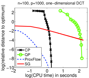
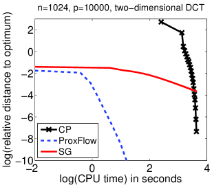
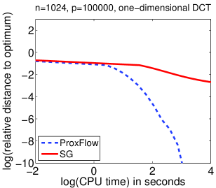
Figure 2: Speed comparisons: distance to the optimal primal value versus CPU time (log-log scale). Due to the computational burden, QP and CP could not be run on every problem.

4.2 Background Subtraction

Following [8], we consider a background subtraction task. Given a sequence of frames from a fixed camera, we try to segment out foreground objects in a new image. If we denote by ${\mathbf{y}}\in\mathbb{R}^{n}$ this image composed of $n$ pixels, we model ${\mathbf{y}}$ as a sparse linear combination of $p$ other images ${\mathbf{X}}\in\mathbb{R}^{n\times p}$, plus an error term ${\mathbf{e}}$ in $\mathbb{R}^{n}$, i.e., ${\mathbf{y}}\approx{\mathbf{X}}{\mathbf{w}}+{\mathbf{e}}$ for some sparse vector ${\mathbf{w}}$ in $\mathbb{R}^{p}$. This approach is reminiscent of [30] in the context of face recognition, where ${\mathbf{e}}$ is further made sparse to deal with small occlusions. The term ${\mathbf{X}}{\mathbf{w}}$ accounts for background parts present in both ${\mathbf{y}}$ and ${\mathbf{X}}$, while ${\mathbf{e}}$ contains specific, or foreground, objects in ${\mathbf{y}}$. The resulting optimization problem is $\min_{{\mathbf{w}},{\mathbf{e}}}\frac{1}{2}\|{\mathbf{y}}\!-\!{\mathbf{X}}{\mathbf{w}}\!-\!{\mathbf{e}}\|_{2}^{2}+\lambda_{1}\|{\mathbf{w}}\|_{1}+\lambda_{2}\|{\mathbf{e}}\|_{1},\ \text{with}\ \lambda_{1},\lambda_{2}\geq 0.$ In this formulation, the $\ell_{1}$-norm penalty on ${\mathbf{e}}$ does not take into account the fact that neighboring pixels in ${\mathbf{y}}$ are likely to share the same label (background or foreground), which may lead to scattered pieces of foreground and background regions (Figure 3). We therefore put an additional structured regularization term $\Omega$ on ${\mathbf{e}}$, where the groups in $\mathcal{G}$ are all the overlapping $3\!\times\!3$-squares on the image. A dataset with hand-segmented evaluation images is used to illustrate the effect of $\Omega$. For simplicity, we use a single regularization parameter, i.e., $\lambda_{1}=\lambda_{2}$, chosen to maximize the number of pixels matching the ground truth. We consider $p=200$ images with $n=57600$ pixels (i.e., a resolution of $120\!\times\!160$, times 3 for the RGB channels). As shown in Figure 3, adding $\Omega$ improves the background subtraction results for the two tested images, by removing the scattered artifacts due to the lack of structural constraints of the $\ell_{1}$-norm, which encodes neither spatial nor color consistency.

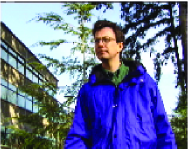
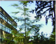
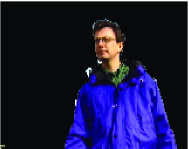
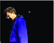
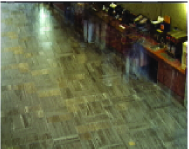
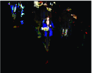
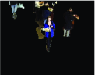
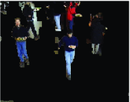
Figure 3: The original image ${\mathbf{y}}$ (column 1), the background (i.e., ${\mathbf{X}}{\mathbf{w}}$) reconstructed by our method (column 2), and the foreground (i.e., the sparsity pattern of ${\mathbf{e}}$ as a mask on the original image) detected with $\ell_{1}$ (column 3) and with $\ell_{1}+\Omega$ (column 4). The rightmost column is another foreground found with $\Omega$, on a different image, with the same values of $\lambda_{1},\lambda_{2}$ as for the previous image. For the top left image, the percentage of pixels matching the ground truth is 98.8% with $\Omega$, 87.0% without. As for the bottom left image, the result is 93.8% with $\Omega$, 90.4% without (best seen in color).

4.3 Multi-Task Learning of Hierarchical Structures

In [11], Jenatton et al. have recently proposed to use a hierarchical structured norm to learn dictionaries of natural image patches. Following their work, we seek to represent $n$ signals $\{{\mathbf{y}}^{1},\dots,{\mathbf{y}}^{n}\}$ of dimension $m$ as sparse linear combinations of elements from a dictionary ${\mathbf{X}}=[{\mathbf{x}}^{1},\ldots,{\mathbf{x}}^{p}]$ in ${\mathbb{R}}^{m\times p}$. This can be expressed for all $i$ in $[1;n]$ as ${\mathbf{y}}^{i}\approx{\mathbf{X}}{\mathbf{w}}^{i}$, for some sparse vector ${\mathbf{w}}^{i}$ in $\mathbb{R}^{p}$. In [11], the dictionary elements are embedded in a predefined tree $\mathcal{T}$, via a particular instance of the structured norm $\Omega$, which we refer to it as $\Omega_{\text{tree}}$, and call ${\mathcal{G}}$ the underlying set of groups. In this case, each signal ${\mathbf{y}}^{i}$ admits a sparse decomposition in the form of a subtree of dictionary elements.

Inspired by ideas from multi-task learning [16], we propose to learn the tree structure $\mathcal{T}$ by pruning irrelevant parts of a larger initial tree $\mathcal{T}_{0}$. We achieve this by using an additional regularization term $\Omega_{\text{joint}}$ across the different decompositions, so that subtrees of $\mathcal{T}_{0}$ will simultaneously be removed for all signals ${\mathbf{y}}^{i}$. In other words, the approach of [11] is extended by the following formulation:

$$\min_{{\mathbf{X}},{\mathbf{W}}}\frac{1}{n}\sum_{i=1}^{n}\!\Big{[}\frac{1}{2}\|{\mathbf{y}}^{i}-{\mathbf{X}}{\mathbf{w}}^{i}\|_{2}^{2}+\lambda_{1}\Omega_{\text{tree}}({\mathbf{w}}^{i})\Big{]}\!+\!\lambda_{2}\Omega_{\text{joint}}({\mathbf{W}}),\ \text{s.t.}\ \|{\mathbf{x}}^{j}\|_{2}\leq 1,~{}\text{for all}~{}j~{}\text{in}~{}[1;p],$$ (6)

where ${\mathbf{W}}\triangleq[{\mathbf{w}}^{1},\ldots,{\mathbf{w}}^{n}]$ is the matrix of decomposition coefficients in ${\mathbb{R}}^{p\times n}$. The new regularization term operates on the rows of ${\mathbf{W}}$ and is defined as $\Omega_{\text{joint}}({\mathbf{W}})\triangleq\sum_{g\in\mathcal{G}}\max_{i\in[1;n]}|{\mathbf{w}}_{g}^{i}|$. The overall penalty on ${\mathbf{W}}$, which results from the combination of $\Omega_{\text{tree}}$ and $\Omega_{\text{joint}}$, is itself an instance of $\Omega$ with general overlapping groups, as defined in Eq (2).

To address problem (6), we use the same optimization scheme as [11], i.e., alternating between ${\mathbf{X}}$ and ${\mathbf{W}}$, fixing one variable while optimizing with respect to the other. The task we consider is the denoising of natural image patches, with the same dataset and protocol as [11]. We study whether learning the hierarchy of the dictionary elements improves the denoising performance, compared to standard sparse coding (i.e., when $\Omega_{\text{tree}}$ is the $\ell_{1}$-norm and $\lambda_{2}=0$) and the hierarchical dictionary learning of [11] based on predefined trees (i.e., $\lambda_{2}=0$). The dimensions of the training set — $50\,000$ patches of size $8\!\times\!8$ for dictionaries with up to $p=400$ elements — impose to handle extremely large graphs, with $|E|\approx|V|\approx 4.10^{7}$. Since problem (6) is too large to be solved exactly sufficiently many times to select the regularization parameters $(\lambda_{1},\lambda_{2})$ rigorously, we use the following heuristics: we optimize mostly with the currently pruned tree held fixed (i.e., $\lambda_{2}=0$), and only prune the tree (i.e., $\lambda_{2}>0$) every few steps on a random subset of $10\,000$ patches. We consider the same hierarchies as in [11], involving between $30$ and $400$ dictionary elements. The regularization parameter $\lambda_{1}$ is selected on the validation set of $25\,000$ patches, for both sparse coding (Flat) and hierarchical dictionary learning (Tree). Starting from the tree giving the best performance (in this case the largest one, see Figure 4), we solve problem (6) following our heuristics, for increasing values of $\lambda_{2}$. As shown in Figure 4, there is a regime where our approach performs significantly better than the two other compared methods. The standard deviation of the noise is $0.2$ (the pixels have values in $[0,1]$); no significant improvements were observed for lower levels of noise.

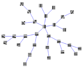
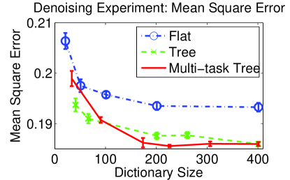
Figure 4: Left: Hierarchy obtained by pruning a larger tree of $76$ elements. Right: Mean square error versus dictionary size. The error bars represent two standard deviations, based on three runs.

5 Conclusion

We have presented a new optimization framework for solving sparse structured problems involving sums of $\ell_{\infty}$-norms of any (overlapping) groups of variables. Interestingly, this sheds new light on connections between sparse methods and the literature of network flow optimization. In particular, the proximal operator for the formulation we consider can be cast as a quadratic min-cost flow problem, for which we propose an efficient and simple algorithm. This allows the use of accelerated gradient methods. Several experiments demonstrate that our algorithm can be applied to a wide class of learning problems, which have not been addressed before within sparse methods.

Appendix A Equivalence to Canonical Graphs

Formally, the notion of equivalence between graphs can be summarized by the following lemma:

Lemma 2 (Equivalence to canonical graphs.)

Let $G=(V,E,s,t)$ be the canonical graph corresponding to a group structure ${\mathcal{G}}$ with weights $(\eta_{g})_{g\in{\mathcal{G}}}$. Let $G^{\prime}=(V,E^{\prime},s,t)$ be a graph sharing the same set of vertices, source and sink as $G$, but with a different arc set $E^{\prime}$. We say that $G^{\prime}$ is equivalent to $G$ if and only if the following conditions hold:

• Arcs of $E^{\prime}$ outgoing from the source are the same as in $E$, with the same costs and capacities.

• Arcs of $E^{\prime}$ going to the sink are the same as in $E$, with the same costs and capacities.

• For every arc $(g,j)$ in $E$, with $(g,j)$ in $V_{gr}\times V_{u}$, there exists a unique path in $E^{\prime}$ from $g$ to $j$ with zero costs and infinite capacities on every arc of the path.

• Conversely, if there exists a path in $E^{\prime}$ between a vertex $g$ in $V_{gr}$ and a vertex $j$ in $V_{u}$, then there exists an arc $(g,j)$ in $E$.

Then, the cost of the optimal min-cost flow on $G$ and $G^{\prime}$ are the same. Moreover, the values of the optimal flow on the arcs $(j,t)$, $j$ in $V_{u}$, are the same on $G$ and $G^{\prime}$.

Proof.  We first notice that on both $G$ and $G^{\prime}$, the cost of a flow on the graph only depends on the flow on the arcs $(j,t)$, $j$ in $V_{u}$, which we have denoted by ${\boldsymbol{\bar{\xi}}}$ in $E$.

We will prove that finding a feasible flow $\pi$ on $G$ with a cost $c(\pi)$ is equivalent to finding a feasible flow $\pi^{\prime}$ on $G^{\prime}$ with the same cost $c(\pi)=c(\pi^{\prime})$. We now use the concept of path flow, which is a flow vector in $G$ carrying the same positive value on every arc of a directed path between two nodes of $G$. It intuitively corresponds to sending a positive amount of flow along a path of the graph.

According to the definition of graph equivalence introduced in the Lemma, it is easy to show that there is a bijection between the arcs in $E$, and the paths in $E^{\prime}$ with positive capacities on every arc. Given now a feasible flow $\pi$ in $G$, we build a feasible flow $\pi^{\prime}$ on $G^{\prime}$ which is a sum of path flows. More precisely, for every arc $a$ in $E$, we consider its equivalent path in $E^{\prime}$, with a path flow carrying the same amount of flow as $a$. Therefore, each arc $a^{\prime}$ in $E^{\prime}$ has a total amount of flow that is equal to the sum of the flows carried by the path flows going over $a^{\prime}$. It is also easy to show that this construction builds a flow on $G^{\prime}$ (capacity and conservation constraints are satisfied) and that this flow $\pi^{\prime}$ has the same cost as $\pi$, that is, $c(\pi)=c(\pi^{\prime})$.

Conversely, given a flow $\pi^{\prime}$ on $G^{\prime}$, we use a classical path flow decomposition (see Proposition 1.1 in [26]), saying that there exists a decomposition of $\pi^{\prime}$ as a sum of path flows in $E^{\prime}$. Using the bijection described above, we know that each path in the previous sums corresponds to a unique arc in $E$. We now build a flow $\pi$ in $G$, by associating to each path flow in the decomposition of $\pi^{\prime}$, an arc in $E$ carrying the same amount of flow. The flow of every other arc in $E$ is set to zero. It is also easy to show that this builds a valid flow in $G$ that has the same cost as $\pi^{\prime}$.  

Appendix B Convergence Analysis

We show in this section the correctness of Algorithm 1 for computing the proximal operator, and of Algorithm 2 for computing the dual norm $\Omega^{\star}$.

B.1 Computation of the Proximal Operator

We now prove that our algorithm converges and that it finds the optimal solution of the proximal problem. This requires that we introduce the optimality conditions for problem (4) derived in [11], since our convergence proof essentially checks that these conditions are satisfied upon termination of the algorithm.

Lemma 3 (Optimality conditions of the problem (4), [11])

The primal-dual variables $({\mathbf{w}},{\boldsymbol{\xi}})$ are respectively solutions of the primal (3) and dual problems (4) if and only if the dual variable ${\boldsymbol{\xi}}$ is feasible for the problem (4) and

$$\begin{split}&{\textstyle{\mathbf{w}}={\mathbf{u}}-\sum_{g\in\mathcal{G}}{\boldsymbol{\xi}}^{g}},\\ &\forall g\in\mathcal{G},~{}~{}\left\{\begin{array}[]{l}{\mathbf{w}}_{g}^{\top}{\boldsymbol{\xi}}_{g}^{g}=\|{\mathbf{w}}_{g}\|_{\infty}\|{\boldsymbol{\xi}}^{g}\|_{1}~{}~{}\text{and}~{}~{}\|{\boldsymbol{\xi}}^{g}\|_{1}=\lambda\eta_{g},\\ \text{or}~{}~{}{\mathbf{w}}_{g}=0.\end{array}\right.\end{split}$$

Note that these optimality conditions provide an intuitive view of our min-cost flow problem. Solving the min-cost flow problem is equivalent to sending the maximum amount of flow in the graph under the capacity constraints, while respecting the rule that the flow outgoing from a group $g$ should always be directed to the variables ${\mathbf{u}}_{j}$ with maximum residual ${\mathbf{u}}_{j}-\sum_{g\in\mathcal{G}}{\boldsymbol{\xi}}^{g}_{j}$.

Before proving the convergence and correctness of our algorithm, we also recall classical properties of the min capacity cuts, which we intensively use in the proofs of this paper. The procedure computeFlow of our algorithm finds a minimum $(s,t)$-cut of a graph $G=(V,E,s,t)$, dividing the set $V$ into two disjoint parts $V^{+}$ and $V^{-}$. $V^{+}$ is by construction the sets of nodes in $V$ such that there exists a non-saturating path from $s$ to $V$, while all the paths from $s$ to $V^{-}$ are saturated. Conversely, arcs from $V^{+}$ to $t$ are all saturated, whereas there can be non-saturated arcs from $V^{-}$ to $t$. Moreover, the following properties hold

• There is no arc going from $V^{+}$ to $V^{-}$. Otherwise the value of the cut would be infinite. (Arcs inside $V$ have infinite capacity by construction of our graph).

• There is no flow going from $V^{-}$ to $V^{+}$ (see properties of the minimum $(s,t)$-cut [26]).

• The cut goes through all arcs going from $V^{+}$ to $t$, and all arcs going from $s$ to $V^{-}$.

All these properties are illustrated on Figure 5.

Figure 5: Cut computed by our algorithm. $V^{+}\!=\!V_{u}^{+}\cup V_{gr}^{+}$, with $V_{gr}^{+}\!=\!\{g\}$, $V_{u}^{+}\!=\!\{1,2\}$, and $V^{-}\!=\!V_{u}^{-}\cup V_{gr}^{-}$, with $V_{gr}^{-}\!=\!\{h\}$, $V_{u}^{-}\!=\!\{3\}$. Arcs going from $s$ to $V^{-}$ are saturated, as well as arcs going from $V^{+}$ to $t$. Saturated arcs are in bold. Arcs with zero flow are dotted.

Recall that we assume (cf. Section 3.1) that the scalars ${\mathbf{u}}_{j}$ are all non negative, and that we add non-negativity constraints on ${\boldsymbol{\xi}}$. With the optimality conditions of Lemma 3 in hand, we can show our first convergence result.

Proposition 1 (Convergence of Algorithm 1)

Algorithm 1 converges in a finite and polynomial number of operations.

Proof.  Our algorithm splits recursively the graph into disjoints parts and processes each part recursively. The processing of one part requires an orthogonal projection onto an $\ell_{1}$-ball and a max-flow algorithm, which can both be computed in polynomial time. To prove that the procedure converges, it is sufficient to show that when the procedure computeFlow is called for a graph $(V,E,s,t)$ and computes a cut $(V^{+},V^{-})$, then the components $V^{+}$ and $V^{-}$ are both non-empty.

Suppose for instance that $V^{-}\!\!=\emptyset$. In this case, the capacity of the min-cut is equal to $\sum_{j\in V_{u}}{\boldsymbol{\gamma}}_{j}$, and the value of the max-flow is $\sum_{j\in V_{u}}{\boldsymbol{\bar{\xi}}}_{j}$. Using the classical max-flow/min-cut theorem [25], we have equality between these two terms. Since, by definition of both ${\boldsymbol{\gamma}}$ and ${\boldsymbol{\bar{\xi}}}$, we have for all $j$ in $V_{u}$, ${\boldsymbol{\bar{\xi}}}_{j}\leq{\boldsymbol{\gamma}}_{j}$, we obtain a contradiction with the existence of $j$ in $V_{u}$ such that ${\boldsymbol{\bar{\xi}}}_{j}\neq{\boldsymbol{\gamma}}_{j}$.

Conversely, suppose now that $V^{+}\!\!=\emptyset$. Then, the value of the max-flow is still $\sum_{j\in V_{u}}{\boldsymbol{\bar{\xi}}}_{j}$, and the value of the min-cut is $\lambda\sum_{g\in V_{gr}}\eta_{g}$. Using again the max-flow/min-cut theorem, we have that $\sum_{j\in V_{u}}{\boldsymbol{\bar{\xi}}}_{j}=\lambda\sum_{g\in V_{gr}}\eta_{g}$. Moreover, by definition of ${\boldsymbol{\gamma}}$, we also have $\sum_{j\in V_{u}}{\boldsymbol{\bar{\xi}}}_{j}\leq\sum_{j\in V_{u}}{\boldsymbol{\gamma}}_{j}\leq\lambda\sum_{g\in V_{gr}}\eta_{g}$, leading to a contradiction with the existence of $j$ in $V_{u}$ such that ${\boldsymbol{\bar{\xi}}}_{j}\neq{\boldsymbol{\gamma}}_{j}$. This proof holds for any graph that is equivalent to the canonical one.  
After proving the convergence, we prove that the algorithm is correct with the next proposition.

Proposition 2 (Correctness of Algorithm 1)

Algorithm 1 solves the proximal problem of Eq. (3).

Proof.  For a group structure ${\mathcal{G}}$, we first prove the correctness of our algorithm if the graph used is its associated canonical graph that we denote $G_{0}=(V_{0},E_{0},s,t)$. We proceed by induction on the number of nodes of the graph. The induction hypothesis ${\mathcal{H}}(k)$ is the following: 
For all canonical graphs $G=(V=V_{u}\cup V_{gr},E,s,t)$ associated with a group structure ${\mathcal{G}}_{V}$ with weights $(\eta_{g})_{g\in{\mathcal{G}}_{V}}$ such that $|V|\leq k$, computeFlow$(V,E)$ solves the following optimization problem:

$$\min_{({\boldsymbol{\xi}}_{j}^{g})_{j\in V_{u},g\in V_{gr}}}\sum_{j\in V_{u}}\frac{1}{2}({\mathbf{u}}_{j}-\sum_{g\in V_{gr}}{\boldsymbol{\xi}}_{j}^{g})^{2}~{}~{}\text{s.t.}~{}~{}\forall g\in V_{gr},~{}\sum_{j\in V_{u}}{\boldsymbol{\xi}}_{j}^{g}\leq\lambda\eta_{g}~{}~{}\text{and}~{}~{}{\boldsymbol{\xi}}_{j}^{g}=0,~{}\forall j\notin g.$$ (7)

Since ${\mathcal{G}}_{V_{0}}={\mathcal{G}}$, it is sufficient to show that ${\mathcal{H}}(|V_{0}|)$ to prove the proposition.

We initialize the induction by ${\mathcal{H}}(2)$, corresponding to the simplest canonical graph, for which $|V_{gr}|=|V_{u}|=1$). Simple algebra shows that ${\mathcal{H}}(2)$ is indeed correct.

We now suppose that ${\mathcal{H}}(k^{\prime})$ is true for all $k^{\prime}<k$ and consider a graph $G=(V,E,s,t)$, $|V|=k$. The first step of the algorithm computes the variable $({\boldsymbol{\gamma}}_{j})_{j\in V_{u}}$ by a projection on the $\ell_{1}$-ball. This is itself an instance of the dual formulation of Eq. (4) in a simple case, with one group containing all variables. We can therefore use Lemma 3 to characterize the optimality of $({\boldsymbol{\gamma}}_{j})_{j\in V_{u}}$, which yields

$$\!\!\left\{\begin{array}[]{l}\sum_{j\in V_{u}}({\mathbf{u}}_{j}-{\boldsymbol{\gamma}}_{j}){\boldsymbol{\gamma}}_{j}=\big{(}\max_{j\in V_{u}}|{\mathbf{u}}_{j}-{\boldsymbol{\gamma}}_{j}|\big{)}\sum_{j\in V_{u}}{\boldsymbol{\gamma}}_{j}~{}\text{and}~{}\sum_{j\in V_{u}}{\boldsymbol{\gamma}}_{j}=\lambda\sum_{g\in V_{gr}}\eta_{g},\!\!\!\!\\ \text{or}~{}~{}{\mathbf{u}}_{j}-{\boldsymbol{\gamma}}_{j}=0,~{}\forall j\in V_{u}.\end{array}\right.$$ (8)

The algorithm then computes a max-flow, using the scalars ${\boldsymbol{\gamma}}_{j}$ as capacities, and we now have two possible situations:

1. If ${\boldsymbol{\bar{\xi}}}_{j}={\boldsymbol{\gamma}}_{j}$ for all $j$ in $V_{u}$, the algorithm stops; we write ${\mathbf{w}}_{j}={\mathbf{u}}_{j}-{\boldsymbol{\bar{\xi}}}_{j}$ for $j$ in $V_{u}$, and using Eq. (8), we obtain

   $$\left\{\begin{array}[]{l}\sum_{j\in V_{u}}{\mathbf{w}}_{j}{\boldsymbol{\bar{\xi}}}_{j}=(\max_{j\in V_{u}}|{\mathbf{w}}_{j}|)\sum_{j\in V_{u}}{\boldsymbol{\bar{\xi}}}_{j}~{}~{}\text{and}~{}~{}\sum_{j\in V_{u}}{\boldsymbol{\bar{\xi}}}_{j}=\lambda\sum_{g\in V_{gr}}\eta_{g},\\ \text{or}~{}~{}{\mathbf{w}}_{j}=0,~{}\forall j\in V_{u}.\end{array}\right.$$ (9)

   We can rewrite the condition above as

   $$\sum_{g\in V_{gr}}\sum_{j\in g}\!{\mathbf{w}}_{j}{\boldsymbol{\xi}}_{j}^{g}=\sum_{g\in V_{gr}}\!(\max_{j\in V_{u}}|{\mathbf{w}}_{j}|)\!\!\!\sum_{j\in V_{u}}{\boldsymbol{\xi}}_{j}^{g}.$$

   Since all the quantities in the previous sum are positive, this can only hold if for all $g\in V_{gr}$,

   $$\sum_{j\in V_{u}}{\mathbf{w}}_{j}{\boldsymbol{\xi}}_{j}^{g}=(\max_{j\in V_{u}}|{\mathbf{w}}_{j}|)\!\sum_{j\in V_{u}}{\boldsymbol{\xi}}_{j}^{g}.$$

   Moreover, by definition of the max flow and the optimality conditions, we have

   $$\forall g\in V_{gr},\ \sum_{j\in V_{u}}\!{\boldsymbol{\xi}}^{g}_{j}\leq\lambda\eta_{g},\ \text{and}\ \sum_{j\in V_{u}}{\boldsymbol{\bar{\xi}}}_{j}=\lambda\sum_{g\in V_{gr}}\eta_{g},$$

   which leads to

   $$\forall g\in V_{gr},\sum_{j\in V_{u}}\!{\boldsymbol{\xi}}^{g}_{j}=\lambda\eta_{g}.$$

   By Lemma 3, we have shown that the problem (7) is solved.

2. Let us now consider the case where there exists $j$ in $V_{u}$ such that ${\boldsymbol{\bar{\xi}}}_{j}\neq{\boldsymbol{\gamma}}_{j}$. The algorithm splits the vertex set $V$ into two parts $V^{+}$ and $V^{-}$, which we have proven to be non-empty in the proof of Proposition 1. The next step of the algorithm removes all edges between $V^{+}$ and $V^{-}$ (see Figure 5). Processing $(V^{+},E^{+})$ and $(V^{-},E^{-})$ independently, it updates the value of the flow matrix ${\boldsymbol{\xi}}^{g}_{j},\ j\in V_{u},\ g\in V_{gr}$, and the corresponding flow vector ${\boldsymbol{\bar{\xi}}}_{j},\ j\in V_{u}$. As for $V$, we denote by $V^{+}_{u}\triangleq V^{+}\cap V_{u}$, $V^{-}_{u}\triangleq V^{-}\cap V_{u}$ and $V^{+}_{gr}\triangleq V^{+}\cap V_{gr}$, $V^{-}_{gr}\triangleq V^{-}\cap V_{gr}$.

   Then, we notice that $(V^{+},E^{+},s,t)$ and $(V^{-},E^{-},s,t)$ are respective canonical graphs for the group structures ${\mathcal{G}}_{V^{+}}\triangleq\{g\cap V_{u}^{+}\mid g\in V_{gr}\}$, and ${\mathcal{G}}_{V^{-}}\triangleq\{g\cap V_{u}^{-}\mid g\in V_{gr}\}$.

   Writing ${\mathbf{w}}_{j}={\mathbf{u}}_{j}-{\boldsymbol{\bar{\xi}}}_{j}$ for $j$ in $V_{u}$, and using the induction hypotheses ${\mathcal{H}}(|V^{+}|)$ and ${\mathcal{H}}(|V^{-}|)$, we now have the following optimality conditions deriving from Lemma 3 applied on Eq. (7) respectively for the graphs $(V^{+},E^{+})$ and $(V^{-},E^{-})$:

   $$\forall g\in V_{gr}^{+},g^{\prime}\triangleq g\cap V_{u}^{+},~{}\left\{\begin{array}[]{l}{\mathbf{w}}_{g^{\prime}}^{\top}{\boldsymbol{\xi}}_{g^{\prime}}^{g}=\|{\mathbf{w}}_{g^{\prime}}\|_{\infty}\sum_{j\in g^{\prime}}\!{\boldsymbol{\xi}}^{g}_{j}~{}~{}\text{and}~{}~{}\sum_{j\in g^{\prime}}\!{\boldsymbol{\xi}}^{g}_{j}=\lambda\eta_{g},\\ \text{or}~{}~{}{\mathbf{w}}_{g^{\prime}}=0,\\ \end{array}\right.$$ (10)

   and

   $$\forall g\in V_{gr}^{-},g^{\prime}\triangleq g\cap V_{u}^{-},\left\{\begin{array}[]{l}{\mathbf{w}}_{g^{\prime}}^{\top}{\boldsymbol{\xi}}_{g^{\prime}}^{g}=\|{\mathbf{w}}_{g^{\prime}}\|_{\infty}\sum_{j\in g^{\prime}}\!{\boldsymbol{\xi}}^{g}_{j}~{}~{}\text{and}~{}~{}\sum_{j\in g^{\prime}}\!{\boldsymbol{\xi}}^{g}_{j}=\lambda\eta_{g},\\ \text{or}~{}~{}{\mathbf{w}}_{g^{\prime}}=0.\\ \end{array}\right.$$ (11)

   We will now combine Eq. (10) and Eq. (11) into optimality conditions for Eq. (7). We first notice that $g\cap V_{u}^{+}=g$ since there are no arcs between $V^{+}$ and $V^{-}$ in $E$ (see the properties of the cuts discussed before this proposition). It is therefore possible to replace $g^{\prime}$ by $g$ in Eq. (10). We will show that it is possible to do the same in Eq. (11), so that combining these two equations yield the optimality conditions of Eq. (7).

   More precisely, we will show that for all $g\in V_{gr}^{-}$ and $j\in g\cap V_{u}^{+}$, $|{\mathbf{w}}_{j}|\leq\max_{l\in g\cap V_{u}^{-}}|{\mathbf{w}}_{l}|$, in which case $g^{\prime}$ can be replaced by $g$ in Eq. (11). This result is relatively intuitive: $(s,V^{+})$ and $(V^{-},t)$ being an $(s,t)$-cut, all arcs between $s$ and $V^{-}$ are saturated, while there are unsaturated arcs between $s$ and $V^{+}$; one therefore expects the residuals ${\mathbf{u}}_{j}-{\boldsymbol{\bar{\xi}}}_{j}$ to decrease on the $V^{+}$ side, while increasing on the $V^{-}$ side. The proof is nonetheless a bit technical.

   Let us show first that for all $g$ in $V_{gr}^{+}$, $\left\|{\mathbf{w}}_{g}\right\|_{\infty}\leq\max_{j\in V_{u}}|{\mathbf{u}}_{j}-{\boldsymbol{\gamma}}_{j}|$. We split the set $V^{+}$ into disjoint parts:

   $$\begin{split}V_{gr}^{++}&\triangleq\{g\in V_{gr}^{+}~{}~{}\text{s.t.}~{}~{}\left\|{\mathbf{w}}_{g}\right\|_{\infty}\leq\max_{j\in V_{u}}|{\mathbf{u}}_{j}-{\boldsymbol{\gamma}}_{j}|\},\\ V_{u}^{++}&\triangleq\{j\in V_{u}^{+}~{}~{}\text{s.t.}~{}~{}\exists g\in V_{gr}^{++},~{}j\in g\},\\ V_{gr}^{+-}&\triangleq V_{gr}^{+}\setminus V_{gr}^{++}=\{g\in V_{gr}^{+}~{}~{}\text{s.t.}~{}~{}\left\|{\mathbf{w}}_{g}\right\|_{\infty}>\max_{j\in V_{u}}|{\mathbf{u}}_{j}-{\boldsymbol{\gamma}}_{j}|\},\\ V_{u}^{+-}&\triangleq V_{u}^{+}\setminus V_{u}^{++}.\\ \end{split}$$

   As previously, we denote $V^{+-}\!\triangleq V_{u}^{+-}\!\cup V_{gr}^{+-}$ and $V^{++}\triangleq\!\!V_{u}^{++}\cup V_{gr}^{++}$. We want to show that $V_{gr}^{+-}$ is necessarily empty. We reason by contradiction and assume that $V_{gr}^{+-}\neq\varnothing$.

   According to the definition of the different sets above, we observe that no arcs are going from $V^{++}$ to $V^{+-}$, that is, for all $g$ in $V_{gr}^{++}$, $g\cap V_{u}^{+-}=\varnothing$. We observe as well that the flow from $V_{gr}^{+-}$ to $V_{u}^{++}$ is the null flow, because optimality conditions (10) imply that for a group $g$ only nodes $j\in g$ such that ${\mathbf{w}}_{j}=\|{\mathbf{w}}_{g}\|_{\infty}$ receive some flow, which excludes nodes in $V_{u}^{++}$ provided $V_{gr}^{+-}\neq\varnothing$; Combining this fact and the inequality $\sum_{g\in V_{gr}^{+}}\lambda\eta_{g}\geq\sum_{j\in V_{u}^{+}}{\boldsymbol{\gamma}}_{j}$ (which is a direct consequence of the minimum $(s,t)$-cut), we have as well

   $$\sum_{g\in V_{gr}^{+-}}\lambda\eta_{g}\geq\sum_{j\in V_{u}^{+-}}{\boldsymbol{\gamma}}_{j}.$$

   Let $j\in V_{u}^{+-}$, if ${\boldsymbol{\bar{\xi}}}_{j}\neq 0$ then for some $g\in V_{gr}^{+-}$ such that $j$ receives some flow from $g$, which from the optimality conditions (10) implies ${\mathbf{w}}_{j}=\|{\mathbf{w}}_{g}\|_{\infty}$; by definition of $V_{gr}^{+-}$, $\|{\mathbf{w}}_{g}\|_{\infty}>{\mathbf{u}}_{j}-{\boldsymbol{\gamma}}_{j}$. But since at the optimum, ${\mathbf{w}}_{j}={\mathbf{u}}_{j}-{\boldsymbol{\bar{\xi}}}_{j}$, this implies that ${\boldsymbol{\bar{\xi}}}_{j}<{\boldsymbol{\gamma}}_{j}$, and in turn that $\sum_{j\in V_{u}^{+-}}{\boldsymbol{\bar{\xi}}}_{j}=\lambda\sum_{g\in V_{gr}^{+-}}\eta_{g}$. Finally,

   $$\lambda\sum_{g\in V_{gr}^{+-}}\eta_{g}=\sum_{j\in V_{u}^{+-},\,{\boldsymbol{\bar{\xi}}}_{j}\neq 0}{\boldsymbol{\bar{\xi}}}_{j}<\sum_{j\in V_{u}^{+-}}{\boldsymbol{\gamma}}_{j}$$

   and this is a contradiction.

   We now have that for all $g$ in $V_{gr}^{+}$, $\left\|{\mathbf{w}}_{g}\right\|_{\infty}\leq\max_{j\in V_{u}}|{\mathbf{u}}_{j}-{\boldsymbol{\gamma}}_{j}|$. The proof showing that for all $g$ in $V_{gr}^{-}$, $\left\|{\mathbf{w}}_{g}\right\|_{\infty}\geq\max_{j\in V_{u}}|{\mathbf{u}}_{j}-{\boldsymbol{\gamma}}_{j}|,$ uses the same kind of decomposition for $V^{-}$, and follows along similar arguments. We will therefore not detail it.

   To recap, we have shown that for all $g\in V_{gr}^{-}$ and $j\in g\cap V_{u}^{+}$, $|{\mathbf{w}}_{j}|\leq\max_{l\in g\cap V_{u}^{-}}|{\mathbf{w}}_{l}|$. Since there is no flow from $V^{-}$ to $V^{+}$, i.e., ${\boldsymbol{\xi}}_{j}^{g}=0$ for $g$ in $V_{gr}^{-}$ and $j$ in $V_{u}^{+}$, we can now replace the definition of $g^{\prime}$ in Eq. (11) by $g^{\prime}\triangleq g\cap V_{u}$, the combination of Eq. (10) and Eq. (11) gives us optimality conditions for Eq. (7).

The proposition being proved for the canonical graph, we extend it now for an equivalent graph in the sense of Lemma 2. First, we observe that the algorithm gives the same values of ${\boldsymbol{\gamma}}$ for two equivalent graphs. Then, it is easy to see that the value ${\boldsymbol{\bar{\xi}}}$ given by the max-flow, and the chosen $(s,t)$-cut is the same, which is enough to conclude that the algorithm performs the same steps for two equivalent graphs.  

B.2 Computation of the Dual Norm $\Omega^{\star}$

Similarly to the proximal operator, the computation of dual norm $\Omega^{*}$ can itself shown to solve another network flow problem, based on the following variational formulation, which extends a previous result from [5]:

Lemma 4 (Dual formulation of the dual-norm $\Omega^{\star}$.)

Let ${\boldsymbol{\kappa}}\in\mathbb{R}^{p}$. We have

$$\Omega^{*}({\boldsymbol{\kappa}})=\!\!\!\min_{{\boldsymbol{\xi}}\in\mathbb{R}^{p\times|\mathcal{G}|},\tau}\!\!\!\tau\quad\text{s.t.}\quad\sum_{g\in\mathcal{G}}{\boldsymbol{\xi}}^{g}={\boldsymbol{\kappa}},\ \text{and}\ \forall g\in\mathcal{G},\ \|{\boldsymbol{\xi}}^{g}\|_{1}\leq\tau\eta_{g}~{}~{}\text{with}~{}~{}\ {\boldsymbol{\xi}}_{j}^{g}=0\ \text{if}\ j\notin g.$$ (12)

Proof.  By definition of $\Omega^{*}({\boldsymbol{\kappa}})$, we have

$$\Omega^{*}({\boldsymbol{\kappa}})\triangleq\max_{\Omega({\mathbf{z}})\leq 1}{\mathbf{z}}^{\top}{\boldsymbol{\kappa}}.$$

By introducing the primal variables $(\alpha_{g})_{g\in{\mathcal{G}}}\in\mathbb{R}^{|{\mathcal{G}}|}$, we can rewrite the previous maximization problem as

$$\Omega^{*}({\boldsymbol{\kappa}})=\max_{\sum_{g\in{\mathcal{G}}}\!\eta_{g}\alpha_{g}\leq 1}{\boldsymbol{\kappa}}^{\top}{\mathbf{z}},\quad\mbox{ s.t. }\quad\forall\ g\in{\mathcal{G}},\ \|{\mathbf{z}}_{g}\|_{\infty}\leq\alpha_{g},$$

with the additional $|{\mathcal{G}}|$ conic constraints $\|{\mathbf{z}}_{g}\|_{\infty}\leq\alpha_{g}$. This primal problem is convex and satisfies Slater’s conditions for generalized conic inequalities, which implies that strong duality holds [32]. We now consider the Lagrangian $\mathcal{L}$ defined as

$$\mathcal{L}({\mathbf{z}},\alpha_{g},\tau,\gamma_{g},{\boldsymbol{\xi}})={\boldsymbol{\kappa}}^{\top}{\mathbf{z}}+\tau(1\!-\!\!\sum_{g\in{\mathcal{G}}}\!\eta_{g}\alpha_{g})+\sum_{g\in{\mathcal{G}}}\binom{\alpha_{g}}{{\mathbf{z}}_{g}}^{\top}\!\binom{\gamma_{g}}{{\boldsymbol{\xi}}^{g}_{g}},$$

with the dual variables $\{\tau,(\gamma_{g})_{g\in{\mathcal{G}}},{\boldsymbol{\xi}}\}\in\mathbb{R}_{+}\!\times\!\mathbb{R}^{|{\mathcal{G}}|}\!\times\!\mathbb{R}^{p\times|{\mathcal{G}}|}$ such that for all $g\in{\mathcal{G}}$, ${\boldsymbol{\xi}}^{g}_{j}=0\,\mbox{ if }\,j\notin g$ and $\|{\boldsymbol{\xi}}^{g}\|_{1}\leq\gamma_{g}$. The dual function is obtained by taking the derivatives of $\mathcal{L}$ with respect to the primal variables ${\mathbf{z}}$ and $(\alpha_{g})_{g\in{\mathcal{G}}}$ and equating them to zero, which leads to

$$\forall j\in\{1,\dots,p\}, {\boldsymbol{\kappa}}_{j}+\!\!\sum_{g\in{\mathcal{G}}}{\boldsymbol{\xi}}^{g}_{j} =0$$

$$\forall g\in{\mathcal{G}}, \tau\eta_{g}-\gamma_{g} =0.$$

After simplifying the Lagrangian and flipping the sign of ${\boldsymbol{\xi}}$, the dual problem then reduces to

$$\min_{{\boldsymbol{\xi}}\in\mathbb{R}^{p\times|\mathcal{G}|},\tau}\tau\quad\mbox{ s.t. }\begin{cases}\forall j\in\{1,\dots,p\},{\boldsymbol{\kappa}}_{j}=\!\!\sum_{g\in{\mathcal{G}}}{\boldsymbol{\xi}}^{g}_{j}\,\mbox{ and }\,{\boldsymbol{\xi}}^{g}_{j}=0\,\mbox{ if }\,j\notin g,\\ \forall g\in{\mathcal{G}},\|{\boldsymbol{\xi}}^{g}\|_{1}\leq\tau\eta_{g},\end{cases}$$

which is the desired result.  
We now prove that Algorithm 2 is correct.

Proposition 3 (Convergence and correctness of Algorithm 2)

Algorithm 2 computes the value of the dual norm of Eq. (12) in a finite and polynomial number of operations.

Proof.  The convergence of the algorithm only requires to show that the cardinality of $V$ in the different calls of the function computeFlow strictly decreases. Similar arguments to those used in the proof of Proposition 1 can show that each part of the cuts $(V^{+},V^{-})$ are both non-empty. The algorithm thus requires a finite number of calls to a max-flow algorithm and converges in a finite and polynomial number of operations.

Let us now prove that the algorithm is correct for a canonical graph. We proceed again by induction on the number of nodes of the graph. More precisely, we consider the induction hypothesis ${\mathcal{H}}^{\prime}(k)$ defined as: 
for all canonical graphs $G=(V,E,s,t)$ associated with a group structure ${\mathcal{G}}_{V}$ and such that $|V|\leq k$, dualNormAux$(V=V_{u}\cup V_{gr},E)$ solves the following optimization problem:

$$\min_{{\boldsymbol{\xi}},\tau}\tau\quad\text{s.t.}\quad\forall j\in V_{u},{\boldsymbol{\kappa}}_{j}=\sum_{g\in V_{gr}}{\boldsymbol{\xi}}_{j}^{g},\ \text{and}\ \forall g\in V_{gr},\ \sum_{j\in V_{u}}{\boldsymbol{\xi}}^{g}_{j}\leq\tau\eta_{g}~{}~{}\text{with}~{}~{}\ {\boldsymbol{\xi}}_{j}^{g}=0\ \text{if}\ j\notin g.$$ (13)

We first initialize the induction by ${\mathcal{H}}(2)$ (i.e., with the simplest canonical graph, such that $|V_{gr}|=|V_{u}|=1$). Simple algebra shows that ${\mathcal{H}}(2)$ is indeed correct.

We next consider a canonical graph $G=(V,E,s,t)$ such that $|V|=k$, and suppose that ${\mathcal{H}}^{\prime}(k-1)$ is true. After the max-flow step, we have two possible cases to discuss:

1. If ${\boldsymbol{\bar{\xi}}}_{j}={\boldsymbol{\gamma}}_{j}$ for all $j$ in $V_{u}$, the algorithm stops. We know that any scalar $\tau$ such that the constraints of Eq. (13) are all satisfied necessarily verifies $\sum_{g\in V_{gr}}\tau\eta_{g}\geq\sum_{j\in V_{u}}{\boldsymbol{\kappa}}_{j}$. We have indeed that $\sum_{g\in V_{gr}}\tau\eta_{g}$ is the value of an $(s,t)$-cut in the graph, and $\sum_{j\in V_{u}}{\boldsymbol{\kappa}}_{j}$ is the value of the max-flow, and the inequality follows from the max-flow/min-cut theorem [25]. This gives a lower-bound on $\tau$. Since this bound is reached, $\tau$ is necessarily optimal.

2. We now consider the case where there exists $j$ in $V_{u}$ such that ${\boldsymbol{\bar{\xi}}}_{j}\neq{\boldsymbol{\kappa}}_{j}$, meaning that for the given value of $\tau$, the constraint set of Eq. (13) is not feasible for ${\boldsymbol{\xi}}$, and that the value of $\tau$ should necessarily increase. The algorithm splits the vertex set $V$ into two non-empty parts $V^{+}$ and $V^{-}$ and we remark that there are no arcs going from $V^{+}$ to $V^{-}$, and no flow going from $V^{-}$ to $V^{+}$. Since the arcs going from $s$ to $V^{-}$ are saturated, we have that $\sum_{g\in V_{gr}^{-}}\tau\eta_{g}\leq\sum_{j\in V_{u}^{-}}{\boldsymbol{\kappa}}_{j}$. Let us now consider $\tau^{\star}$ the solution of Eq. (13). Using the induction hypothesis ${\mathcal{H}}^{\prime}(|V^{-}|)$, the algorithm computes a new value $\tau^{\prime}$ that solves Eq. (13) when replacing $V$ by $V^{-}$ and this new value satisfies the following inequality $\sum_{g\in V_{gr}^{-}}\tau^{\prime}\eta_{g}\geq\sum_{j\in V_{u}^{-}}{\boldsymbol{\kappa}}_{j}$. The value of $\tau^{\prime}$ has therefore increased and the updated flow ${\boldsymbol{\xi}}$ now satisfies the constraints of Eq. (13) and therefore $\tau^{\prime}\geq\tau^{\star}$. Since there are no arcs going from $V^{+}$ to $V^{-}$, $\tau^{\star}$ is feasible for Eq. (13) when replacing $V$ by $V^{-}$ and we have that $\tau^{\star}\geq\tau^{\prime}$ and then $\tau^{\prime}=\tau^{\star}$.

To prove that the result holds for any equivalent graph, similar arguments to those used in the proof of Proposition 1 can be exploited, showing that the algorithm computes the same values of $\tau$ and same $(s,t)$-cuts at each step.  

Appendix C Algorithm FISTA with duality gap

In this section, we describe in details the algorithm FISTA [4] when applied to solve problem (1), with a duality gap as stopping criterion.

Without loss of generality, let us assume we are looking for models of the form ${\mathbf{X}}{\mathbf{w}}$, for some matrix ${\mathbf{X}}\in\mathbb{R}^{n\times p}$ (typically, linear models where ${\mathbf{X}}$ is the data matrix of $n$ observations). Thus, we can consider the following primal problem

$$\min_{{\mathbf{w}}\in{\mathbb{R}}^{p}}f({\mathbf{X}}{\mathbf{w}})+\lambda\Omega({\mathbf{w}}),$$ (14)

in place of (1). Based on Fenchel duality arguments [29],

$$f({\mathbf{X}}{\mathbf{w}})+\lambda\Omega({\mathbf{w}})+f^{*}(-{\boldsymbol{\kappa}}),\ \text{for}\ {\mathbf{w}}\in\mathbb{R}^{p},{\boldsymbol{\kappa}}\in\mathbb{R}^{n}\ \text{and}\ \Omega^{*}({\mathbf{X}}^{\top}{\boldsymbol{\kappa}})\leq\lambda,$$

is a duality gap for (14). where $f^{*}({\boldsymbol{\kappa}})\triangleq\sup_{{\mathbf{z}}}[{\mathbf{z}}^{\top}{\boldsymbol{\kappa}}-f({\mathbf{z}})]$ is the Fenchel conjugate of $f$. Given a primal variable ${\mathbf{w}}$, a good dual candidate ${\boldsymbol{\kappa}}$ can be obtained by looking at the conditions that have to be satisfied by the pair $({\mathbf{w}},{\boldsymbol{\kappa}})$ at optimality [29]. In particular, the dual variable ${\boldsymbol{\kappa}}$ is chosen to be

$${\boldsymbol{\kappa}}=-\rho^{-1}\nabla\!f({\mathbf{X}}{\mathbf{w}}),\ \text{with}\ \rho\triangleq\max\big{\{}\lambda^{-1}\Omega^{*}({\mathbf{X}}^{\top}\!\nabla\!f({\mathbf{X}}{\mathbf{w}})),1\big{\}}.$$

Consequently, computing the duality gap requires evaluating the dual norm $\Omega^{*}$. We sum up the computation of the duality gap in Algorithm 3.

Moreover, we refer to the proximal operator associated with $\lambda\Omega$ as $\text{prox}_{[\lambda\Omega]}$. As a brief reminder, it is defined as the function that maps the vector ${\mathbf{u}}$ in $\mathbb{R}^{p}$ to the (unique, by strong convexity) solution of Eq. (3).

Algorithm 3 FISTA procedure to solve problem (14).

1:  Inputs: initial ${\mathbf{w}}_{(0)}\in\mathbb{R}^{p}$, $\Omega$, $\lambda>0$, $\varepsilon_{\text{gap}}>0$ (precision for the duality gap).

2:  Parameters: $\nu>1$, $L_{0}>0$.

3:  Outputs: solution ${\mathbf{w}}$.

4:  Initialization: ${\mathbf{y}}_{(1)}={\mathbf{w}}_{(0)}$, $t_{1}=1$, $k=1$.

5:  while  $\big{\{}$ computeDualityGap$\big{(}{\mathbf{w}}_{(k-1)}\big{)}>\varepsilon_{\text{gap}}\big{\}}$  do

6:     Find the smallest integer $s_{k}\!\geq\!0$ such that

7:     $\quad f(\text{prox}_{[\lambda\Omega]}({\mathbf{y}}_{(k)}))\leq f({\mathbf{y}}_{(k)})+\Delta_{(k)}^{\top}\nabla f({\mathbf{y}}_{(k)})+\frac{\tilde{L}}{2}\|\Delta_{(k)}\|_{2}^{2},$

8:        with $\tilde{L}\triangleq L_{k}\nu^{s_{k}}$ and $\Delta_{(k)}\triangleq{\mathbf{y}}_{(k)}\!-\!\text{prox}_{[\lambda\Omega]}({\mathbf{y}}_{(k)})$.

9:     $L_{k}\leftarrow L_{k-1}\nu^{s_{k}}$.

10:     ${\mathbf{w}}_{(k)}\leftarrow\text{prox}_{[\lambda\Omega]}({\mathbf{y}}_{(k)})$.

11:     $t_{k+1}\leftarrow(1+\sqrt{1+t_{k}^{2}})/2$.

12:     ${\mathbf{y}}_{(k+1)}\leftarrow{\mathbf{w}}_{(k)}+\frac{t_{k}-1}{t_{k+1}}({\mathbf{w}}_{(k)}-{\mathbf{w}}_{(k-1)})$.

13:     $k\leftarrow k+1$.

14:  end while

15:  Return: ${\mathbf{w}}\leftarrow{\mathbf{w}}_{(k-1)}$.

Procedure computeDualityGap(${\mathbf{w}}$)

1:  ${\boldsymbol{\kappa}}\leftarrow-\rho^{-1}\nabla\!f({\mathbf{X}}{\mathbf{w}}),\ \text{with}\ \rho\triangleq\max\big{\{}\lambda^{-1}\Omega^{*}({\mathbf{X}}^{\top}\!\nabla\!f({\mathbf{X}}{\mathbf{w}})),1\big{\}}$.

2:  Return: $f({\mathbf{X}}{\mathbf{w}})+\lambda\Omega({\mathbf{w}})+f^{*}(-{\boldsymbol{\kappa}})$.

Appendix D Additional Experimental Results

D.1 Speed comparison of Algorithm 1 with parametric max-flow algorithms

As shown in [19], min-cost flow problems, and in particular, the dual problem of (3), can be reduced to a specific parametric max-flow problem. We thus compare our approach (ProxFlow) with the efficient parametric max-flow algorithm proposed by Gallo, Grigoriadis, and Tar- jan  [22] and a simplified version of the latter proposed by Babenko and Goldberg in  [23]. We refer to these two algorithms as GGT and SIMP respectively. The benchmark is established on the same datasets as those already used in the experimental section of the paper, namely: (1) three datasets built from overcomplete bases of discrete cosine transforms (DCT), with respectively $10^{4},\ 10^{5}$ and $10^{6}$ variables, and (2) images used for the background subtraction task, composed of 57600 pixels. For GGT and SIMP, we use the paraF software which is a C++ parametric max-flow implementation available at http://www.avglab.com/andrew/soft.html. Experiments were conducted on a single-core 2.33 Ghz.

We report in the following table the execution time in seconds of each algorithm, as well as the statistics of the corresponding problems:

Number of variables $p$	$10\,000$	$100\,000$	$1\,000\,000$	$57\,600$
$|V|$	$20\,000$	$200\,000$	$2\,000\,000$	$75\,600$
$|E|$	$110\,000$	$500\,000$	$11\,000\,000$	$579\,632$
ProxFlow (in sec.)	$\mathbf{0.4}$	$\mathbf{3.1}$	$\mathbf{113.0}$	$\mathbf{1.7}$
GGT (in sec.)	$2.4$	$26.0$	$525.0$	$16.7$
SIMP (in sec.)	$1.2$	$13.1$	$284.0$	$8.31$

Although we provide the speed comparison for a single value of $\lambda$ (the one used in the corresponding experiments of the paper), we observed that our approach consistently outperforms GGT and SIMP for values of $\lambda$ corresponding to different regularization regimes.

References

• [1] P. Bickel, Y. Ritov, and A. Tsybakov. Simultaneous analysis of Lasso and Dantzig selector. Ann. Stat., 37(4):1705–1732, 2009.
• [2] B. Efron, T. Hastie, I. Johnstone, and R. Tibshirani. Least angle regression. Ann. Stat., 32(2):407–499, 2004.
• [3] Y. Nesterov. Gradient methods for minimizing composite objective function. Technical report, Center for Operations Research and Econometrics (CORE), Catholic University of Louvain, 2007.
• [4] A. Beck and M. Teboulle. A fast iterative shrinkage-thresholding algorithm for linear inverse problems. SIAM J. Imag. Sci., 2(1):183–202, 2009.
• [5] R. Jenatton, J-Y. Audibert, and F. Bach. Structured variable selection with sparsity-inducing norms. Technical report, 2009. Preprint arXiv:0904.3523v1.
• [6] L. Jacob, G. Obozinski, and J.-P. Vert. Group Lasso with overlap and graph Lasso. In Proc. ICML, 2009.
• [7] P. Zhao, G. Rocha, and B. Yu. The composite absolute penalties family for grouped and hierarchical variable selection. Ann. Stat., 37(6A):3468–3497, 2009.
• [8] J. Huang, Z. Zhang, and D. Metaxas. Learning with structured sparsity. In Proc. ICML, 2009.
• [9] R. G. Baraniuk, V. Cevher, M. Duarte, and C. Hegde. Model-based compressive sensing. IEEE T. Inform. Theory, 2010. to appear.
• [10] S. Kim and E. P. Xing. Tree-guided group lasso for multi-task regression with structured sparsity. In Proc. ICML, 2010.
• [11] R. Jenatton, J. Mairal, G. Obozinski, and F. Bach. Proximal methods for sparse hierarchical dictionary learning. In Proc. ICML, 2010.
• [12] V. Roth and B. Fischer. The Group-Lasso for generalized linear models: uniqueness of solutions and efficient algorithms. In Proc. ICML, 2008.
• [13] R. Tibshirani. Regression shrinkage and selection via the Lasso. J. Roy. Stat. Soc. B, 58(1):267–288, 1996.
• [14] M. Yuan and Y. Lin. Model selection and estimation in regression with grouped variables. J. Roy. Stat. Soc. B, 68:49–67, 2006.
• [15] J. Huang and T. Zhang. The benefit of group sparsity. Technical report, 2009. Preprint arXiv:0901.2962.
• [16] G. Obozinski, B. Taskar, and M. I. Jordan. Joint covariate selection and joint subspace selection for multiple classification problems. Stat. Comput., 20(2):231–252, 2010.
• [17] F. Bach. Exploring large feature spaces with hierarchical multiple kernel learning. In Adv. NIPS, 2008.
• [18] P. L. Combettes and J.-C. Pesquet. Proximal splitting methods in signal processing. In Fixed-Point Algorithms for Inverse Problems in Science and Engineering. Springer, 2010.
• [19] D. S. Hochbaum and S. P. Hong. About strongly polynomial time algorithms for quadratic optimization over submodular constraints. Math. Program., 69(1):269–309, 1995.
• [20] J. Duchi, S. Shalev-Shwartz, Y. Singer, and T. Chandra. Efficient projections onto the $\ell_{1}$-ball for learning in high dimensions. In Proc. ICML, 2008.
• [21] P. Brucker. An O(n) algorithm for quadratic knapsack problems. Oper. Res. Lett., 3:163–166, 1984.
• [22] G. Gallo, M. E. Grigoriadis, and R. E. Tarjan. A fast parametric maximum flow algorithm and applications. SIAM J. Comput., 18:30–55, 1989.
• [23] M. Babenko and A.V. Goldberg. Experimental evaluation of a parametric flow algorithm. Technical report, Microsoft Research, 2006. MSR-TR-2006-77.
• [24] A. V. Goldberg and R. E. Tarjan. A new approach to the maximum flow problem. In Proc. of ACM Symposium on Theory of Computing, pages 136–146, 1986.
• [25] L. R. Ford and D. R. Fulkerson. Maximal flow through a network. Canadian J. Math., 8(3):399–404, 1956.
• [26] D. P. Bertsekas. Linear Network Optimization. MIT Press, 1991.
• [27] B. V. Cherkassky and A. V. Goldberg. On implementing the push-relabel method for the maximum flow problem. Algorithmica, 19(4):390–410, 1997.
• [28] S. Negahban, P. Ravikumar, M. J. Wainwright, and B. Yu. A unified framework for high-dimensional analysis of M-estimators with decomposable regularizers. In Adv. NIPS, 2009.
• [29] J. M. Borwein and A. S. Lewis. Convex analysis and nonlinear optimization: Theory and examples. Springer, 2006.
• [30] J. Wright, A. Y. Yang, A. Ganesh, S. S. Sastry, and Y. Ma. Robust face recognition via sparse representation. IEEE T. Pattern. Anal., 31(2):210–227, 2009.
• [31] P. Sprechmann, I. Ramirez, G. Sapiro, and Y. C. Eldar. Collaborative hierarchical sparse modeling. Technical report, 2010. Preprint arXiv:1003.0400v1.
• [32] S. P. Boyd and L. Vandenberghe. Convex Optimization. Cambridge University Press, 2004.