Poincaré Invariant Quantum Mechanics based on Euclidean Green functions

Abstract

We investigate a formulation of Poincaré invariant quantum mechanics where the dynamical input is Euclidean invariant Green functions or their generating functional. We argue that within this framework it is possible to calculate scattering observables, binding energies, and perform finite Poincaré transformations without using any analytic continuation. We demonstrate, using a toy model, how matrix elements of $e^{-\beta H}$ in normalizable states can be used to compute transition matrix elements for energies up to 2 GeV. We discuss some open problems.

We investigate the possibility of formulating Poincaré invariant quantum models of few-body systems where the dynamical input is given by a set of Euclidean-invariant Green functions. This is an alternative to the direct construction of Poincaré Lie algebras on few-body Hilbert spaces. In the proposed framework all calculations are performed using time Euclidean variables, with no analytic continuation.

One potential advantage of the Euclidean approach is that it has a more direct relation to Lagrangian based field theory models. One of the challenges is the construction of a robust class of suitable model Green functions. In this paper do not address this problem; we assume that this has already been solved and discuss how one can calculate observables without analytic continuation.

Most of what we propose in not new, it is motivated the reconstruction theorem of a quantum theory in Euclidean field theory. The fundamental work was done by Osterwalder and Schrader Osterwalder:1973dx Osterwalder:1974tc . The approach illustrated in this work is strongly motivated by Fröhlich’s Frohlich:1974 elegant solution of the reconstruction problem using generating functionals. One of the interesting observations of Osterwalder and Schrader is that locality is not needed to construct the quantum theory.

To keep our discussion as simple as possible we assume that we are given a Euclidean invariant generating functional for a scalar field theory. This input replaces the model Hamiltonain. We assume that this generating functional is Euclidean invariant, positive, reflection positive, and satisfies space-like cluster properties. These requirements are defined below. The conditions on the generating functional imply conditions on Green functions in models based on a subsets of Green functions.

For a scalar field the Euclidean generating functional $Z[f]$ is the functional Fourier transform of the Euclidean path measure:

$$Z[f]:={\int D_{e}[\phi]e^{-A[\phi]+i\phi(f)}\over\int D_{e}[\phi]e^{-A[\phi]}}=\sum_{n}{(i)^{n}\over n!}S_{n}\underbrace{(f,\cdots,f)}_{\mbox{n times}}.$$ (1)

where $f({\sf x})=f(\tau,\mathbf{x})$ is a test function in four Euclidean space-time variables and $S_{n}({\sf x}_{1},\cdots,{\sf x}_{n})$ is the $n$-point Euclidean Green function.

The generating functional is Euclidean invariant if $Z[f]=Z[f^{\prime}]$ where $f^{\prime}({\sf x})=f(E^{-1}({\sf x}-{\sf a}))$ where ${\sf x}\to E{\sf x}+{\sf a}$ is a four-dimensional Euclidean transformation of the arguments of $f$.

The generating functional is positive if for every finite sequence of real test functions $\{f_{i}\}$ the matrices $E_{ij}=Z[f_{i}-f_{j}]$ are non-negative.

The generating functional is reflection positive if for every sequence $\{f_{i}\}$, of real test functions with support for positive Euclidean time, the matrices $M_{ij}=Z[f_{i}-\Theta f_{j}]$ are non-negative, where $(\Theta f)(\tau,\mathbf{x})=f(-\tau,\mathbf{x})$ is Euclidean time reflection.

The generating functional satisfies space-like cluster properties if

$$\lim_{|\mathbf{a}|\to\infty}\left(Z[f+g_{\mathbf{a}}]-Z[f]Z[g]\right)\to 0$$ (2)

where

$$g_{\mathbf{a}}(\tau,\mathbf{x}):=g(\tau,\mathbf{x}-\mathbf{a}).$$ (3)

These are the primary requirements that are expected of an acceptable generating functional.

I Hilbert Space

We begin by representing vectors by wave functionals of the form

$$B[\phi]=\sum_{j=1}^{N_{b}}b_{j}e^{i\phi(f_{j})}\qquad C[\phi]=\sum_{k=1}^{N_{c}}c_{k}e^{i\phi(g_{k})}$$ (4)

where $b_{j}$ and $c_{k}$ are complex constants and $f_{j}({\sf x})$ and $g_{k}({\sf x})$ are real Euclidean test functions. The argument “$\phi$” plays the role of a formal integration variable.

We define a Euclidean-invariant scalar product of two-wave functionals by

$$(B,C):=\sum_{j=1}^{N_{b}}\sum_{k=1}^{N_{c}}b^{*}_{j}c_{k}Z[g_{k}-f_{j}].$$ (5)

This becomes a Hilbert space inner product by identifying vectors whose difference has zero norm and adding convergent sequences of finite sums. We call this space the Euclidean Hilbert space.

Reflection positivity can be used to define a second Hilbert space. Vectors are represented by wave functionals of the form (4) where the test functions $f_{j}({\sf x})$, $g_{k}({\sf x})$ are restricted to have support for positive Euclidean times. We call these test functions positive-time test functions. We define the physical scalar product of two such wave functionals by

$$\langle B|C\rangle:=\sum_{j=1}^{N_{b}}\sum_{k=1}^{N_{c}}b^{*}_{j}c_{k}Z[g_{k}-\Theta f_{j}].$$ (6)

As in the Euclidean case, this becomes a Hilbert space inner product by identifying vectors whose difference has zero norm and adding convergent sequences of finite sums. We will refer to the resulting Hilbert space as the physical Hilbert space. Reflection positivity is equivalent to the requirement that

$$\langle B|B\rangle\geq 0.$$ (7)

II Poincaré Lie Algebra

Note that the determinant of the $2\times 2$ matrices

$$X=\left(\begin{array}[]{cc}t-z&x-iy\\ x+iy&t+z\end{array}\right)\qquad{\sf X}=\left(\begin{array}[]{cc}i\tau-z&x-iy\\ x+iy&i\tau+z\end{array}\right)$$ (8)

gives the Lorentz and Euclidean invariant distances. The determinants are preserved under the linear transformations $X\to X^{\prime}=AXB^{t}$ and ${\sf X}\to{\sf X}^{\prime}=A{\sf X}B^{t}$ where $A$ and $B$ are complex matrices with determinant 1. These transformations are generally complex but the determinants remain real. It follows that the pair $(A,B)$ equivalently defines both complex Lorentz and complex $O(4)$ transformations. Real Lorentz transformations have $B=A^{*}$ while real $O(4)$ transformations have A and B $\in SU(2)$. In this section we use the observation that real $O(4)$ transformations correspond to complex Lorentz transformations to extract Poincaré generators on the physical Hilbert space.

Finite Euclidean transformations, $T(E,{\sf a})$, act on wave functionals as follows

$$T(E,{\sf a})B[\phi]=\sum_{j=1}^{N_{b}}b_{j}e^{i\phi(f_{E,{\sf a},j})},$$ (9)

where $f_{E,{\sf a},j}({\sf x})=f_{j}(E^{-1}({\sf x}-{\sf a}))$ and $E\in O(4)$. Since real Euclidean transformations preserve the Euclidean scalar product $(\cdot,\cdot)$, $T(E,{\sf a})$ is unitary on the Euclidean Hilbert space.

These same transformations, with restrictions on the domains and group parameters to ensure the positive time support condition is preserved, are defined on the physical Hilbert space, but the resulting transformations are not unitary.

For three-dimensional Euclidean transformations, $T(E,{\sf a})$ maps the physical Hilbert space to the physical Hilbert space in a manner that preserves the physical Hilbert space scalar product. This implies that for space translations and ordinary rotations $T({\sf E},a)$ is unitary on the physical Hilbert space.

Positive Euclidean time translations, $T(I,(\beta,0))$, $\beta>0$, map the physical Hilbert space to the physical Hilbert space, however because of the Euclidean time reversal operator in the physical scalar product, Euclidean time translations are Hermitian, rather than unitary. It is possible to use the unitarity of $\Theta$ on the Euclidean Hilbert space along with reflection positivityglimm:1981 to show that positive Euclidean time evolution is a contractive Hermetian semigroup on the physical Hilbert space.

Rotations in planes that contain the Euclidean time direction do not generally preserve the positive Euclidean time support constraint. However, if the test functions are restricted to have support in a cone with axis of symmetry along the Euclidean time axis that makes an angle less than $\pi/2$ with the time axis, then rotations in space-time planes through angles $\rho$ small enough to leave the cone in the positive-time half plane are defined on this restricted set of wave functionals. On this domain and for this restricted set of angles Euclidean space-time rotations are Hermitian. They form a local symmetric semigroup. What is relevant is that just like one-parameter unitary groups and contractive Hermitian semigroups, local symmetric semigroups have self-adjoint generators Klein:1981 Klein:1983 Frohlich:1983kp .

The result is that on the physical Hilbert space the various one-parameter subgroups of the real Euclidean transformations have the form

$$T(E,{\sf a})\to e^{i\mathbf{a}\cdot\mathbf{P}},e^{i{\mbox{\boldmath$\theta$}}\cdot\mathbf{J}},e^{-\beta H},e^{{\mbox{\boldmath$\rho$}}\cdot\mathbf{K}}$$ (10)

where $H,\mathbf{P},\mathbf{J},\mathbf{K}$ are all self-adjoint operators on the physical Hilbert space. It can also be shown by direct calculation that the infinitesimal generators satisfy the Poincaré commutation relations. This is a consequence of the relation between the complex Lorentz and complex $O(4)$ groups.

Matrix elements of the generators can be computed by differentiating $T(E,{\sf a})$ with respect to the group parameters:

$$\langle B|\mathbf{J}|C\rangle=-i{\partial\over\partial\mbox{\boldmath$\theta$}}\sum_{j=1}^{N_{b}}\sum_{k=1}^{N_{c}}b^{*}_{j}c_{k}Z[g_{k}-\Theta f_{E(\mbox{\boldmath$\theta$}),0,j}]_{|_{\mbox{\boldmath$\theta$}=0}}$$ (11)

$$\langle B|\mathbf{P}|C\rangle=-i{\partial\over\partial\mathbf{a}}\sum_{j=1}^{N_{b}}\sum_{k=1}^{N_{c}}b^{*}_{j}c_{k}Z[g_{k}-\Theta f_{I,\mathbf{a},j}]_{|_{\mathbf{a}=0}}$$ (12)

$$\langle B|{H}|C\rangle=-{\partial\over\partial\beta}\sum_{j=1}^{N_{b}}\sum_{k=1}^{N_{c}}b^{*}_{j}c_{k}Z[g_{k}-\Theta f_{I,(\beta,0),j}]_{|_{\beta=0}}$$ (13)

$$\langle B|\mathbf{K}|C\rangle={\partial\over\partial\mbox{\boldmath$\rho$}}\sum_{j=1}^{N_{b}}\sum_{k=1}^{N_{c}}b^{*}_{j}c_{k}Z[g_{k}-\Theta f_{E(\mbox{\boldmath$\rho$}),0,j}]_{|_{\beta=0}}$$ (14)

where $\rho$ is the axis and angle of a rotation in a plane containing the Euclidean time direction (it is an imaginary rapidity).

In this section we have illustrated how the Poincaré generators can be constructed directly from the Euclidean generating functional without using any analytic continuation.

III Particles

Particles are associated with eigenstates of the mass Casimir operator of the Poincaré group with eigenvalues in the point spectrum. Matrix elements of the square of the mass operator are

$$\langle B|M^{2}|C\rangle=\left({\partial^{2}\over\partial\beta^{2}}+{\partial^{2}\over\partial\mathbf{a}^{2}}\right)\sum_{j=1}^{N_{b}}\sum_{k=1}^{N_{c}}b^{*}_{j}c_{k}Z[g_{k}-\Theta f_{I,(\beta,\mathbf{a}),j}]_{|_{\mathbf{a}=\beta=0}}$$ (15)

Since the positive-time wave functionals are dense in the physical Hilbert space it is possible to construct an orthonormal basis of wave functionals $\{B_{n}[\phi]\}$ satisfying

$$B_{n}[\phi]\qquad\langle B_{n}|B_{m}\rangle=\delta_{mn}.$$ (16)

Point eigenstates of the mass operator are normalizable solutions of the eigenvalue problem

$$\left((M^{2}-\lambda^{2})B_{\lambda}\right)[\phi]=0.$$ (17)

In the orthonormal basis $\{B_{n}[\phi]\}$ this eigenvalue equation becomes

$$B_{\lambda}[\phi]=\sum_{n}b_{n}B_{n}[\phi]\qquad\sum_{n}\langle B_{m}|M^{2}|B_{n}\rangle b_{n}=\lambda^{2}b_{m}$$ (18)

where the sum is generally infinite.

States of sharp linear momentum and canonical spin can be extracted using translations and rotations. Specifically mass-momentum eigenstates are given by

$$\langle C|B_{\lambda}(\mathbf{p})\rangle=\int{d^{3}a\over(2\pi)^{3/2}}e^{-i\mathbf{p}\cdot\mathbf{a}}\sum_{j=1}^{N_{c}}\sum_{n}b_{n}c^{*}_{j}Z[f_{I,(0,\mathbf{a}),n}-\Theta g_{j}]$$ (19)

which can be normalized so

$$\langle B_{\lambda}(\mathbf{p}\,^{\prime})|B_{\lambda}(\mathbf{p})\rangle=\delta(\mathbf{p}^{\prime}-\mathbf{p})$$ (20)

Similarly, it is possible find simultaneous eigenstates of mass, linear momentum and spin using

$$\langle C|B_{\lambda,j}(\mathbf{p},\mu)\rangle:=\int_{SU(2)}\sum_{\nu=-j}^{j}dR\langle C|T(R,0)|B_{\lambda}(R^{-1}\mathbf{p})\rangle D^{j*}_{\mu\nu}(R)$$ (21)

where $dR$ is the $SU(2)$ Haar measure.

The wave functional $B_{\lambda,j}(\mathbf{p},\mu)[\phi]$ describes a particle of mass $\lambda$, linear momentum $\mathbf{p}$, spin $j$ and z-component of canonical spin $\mu$.

We remark that if this state is non-degenerate, then it must transform irreducibly with respect to the Poincaré group. This means that

$$\langle C|U(\Lambda,a)|B_{\lambda,j}(\mathbf{p},\mu)\rangle:=\sum_{\mu^{\prime}=-j}^{j}\int d\mathbf{p}^{\prime}\langle C|B_{\lambda,j}(\mathbf{p}^{\prime},\mu^{\prime})\rangle{\cal D}^{\lambda,j}_{\mathbf{p}^{\prime}\mu^{\prime};\mathbf{p},\mu}[\Lambda,a]$$ (22)

where

$${\cal D}^{\lambda,j}_{\mathbf{p}^{\prime}\mu^{\prime};\mathbf{p},\mu}[\Lambda,a]:=\langle(\lambda,j),\mathbf{p^{\prime}},\mu^{\prime}|U[\Lambda,a]|(\lambda,j),\mathbf{p},\mu\rangle$$ (23)

is the known Wigner fucntion of the Poincaré group in the basis $|(\lambda,j),\mathbf{p},\mu\rangle$.

As emphasized in the previous sections, all of the calculations were done using Euclidean Green functions and test functions, with no analytic continuation. Equation (22) demonstrates how to perform finite Poincaré transformation on the one-body solutions.

IV Scattering

The conventional treatment of scattering problems in quantum field theory is formulated using the LSZ asymptotic conditions. These have the advantage that they can be implemented without solving the one-body problem, which is non-trivial in field theories. However, given one-body solutions it is also possible to formulate scattering asymptotic conditions using strong limits. These asymptotic conditions were given by Hagg and Ruelle Haag:1958vt Ruelle:1962 , and they are the most natural generalization of the formulation of scattering that is used in non-relativistic quantum mechanics.

In this work it is useful to use a two Hilbert space formulation Coester:1965 of Haag-Ruelle scattering theorysimon baumgartl:1983 , where an asymptotic Hilbert space is introduced the formulate the asymptotic conditions on the scattering states. All particles appear as elementary particles in the asymptotic space; the internal structure (bound-state wave functions) appear in the mapping to the physical Hilbert space.

For a scalar field theory with a mass eigenstate with eigenvalue $\lambda$, Haag and Ruelle multiply the Fourier transform of the field by a smooth function $\rho_{\lambda}(p^{2})$ that is $1$ when $p^{2}=-\lambda^{2}$ and vanishes when $-p^{2}$ is in rest of the mass spectrum of the system. The product, $\tilde{\phi}_{\rho}(p):=\tilde{\phi}(p)\rho_{\lambda}(p^{2})$, is Fourier transformed back to configuration space. The resulting field, $\phi_{\rho}(x)$, has the property that it creates a one-body state of mass $\lambda$ out of the vacuum. It transforms covariantly, but is no longer local. While this is not a free field, it asymptotically looks like a free field, and it is useful to extract the linear combination of $\phi_{\rho}(x)$ and $\dot{\phi}_{\rho}(x)$ that asymptotically becomes the creation part of the field:

$$A(f,t):=-i\int\phi_{\rho}(x)\stackrel{{\scriptstyle\leftrightarrow}}{{\partial_{0}}}f(x)d\mathbf{x}$$ (24)

where $f(x)$ is a positive-energy solution of the Klein Gordon equation with mass $\lambda$. Haag and Ruelle prove that the scattering states of the theory are given by the limits:

$$\lim_{t\to\pm\infty}\||\Psi_{\pm}(f_{1},\cdots f_{n})\rangle-A(f_{n},t)\cdots A(f_{1},t)|0\rangle\|=0.$$ (25)

To express this in a two Hilbert space notation we rewrite $A(f,t)$ as

$$A(f,t)|0\rangle=e^{iHt}\int\underbrace{\left([H,\hat{\phi}_{\rho}(\mathbf{p})]-\omega_{\lambda}(\mathbf{p})\hat{\phi}_{\rho}(\mathbf{p})\right)}_{A(\mathbf{p})}e^{-iHt}|0\rangle d\mathbf{p}e^{-i\omega_{\lambda}(\mathbf{p})t}\tilde{f}(\mathbf{p})d\mathbf{p}.$$ (26)

It follows that

$$A(f_{n},t)\cdots A(f_{1},t)|0\rangle=e^{iHt}\int\underbrace{A(\mathbf{p}_{n})\cdots A(\mathbf{p}_{1})|0\rangle}_{\Phi:\otimes{\cal H}_{i}\to{\cal H}}d\mathbf{p}_{n}\cdots d\mathbf{p}_{1}e^{-iH_{0}t}f_{n}(\mathbf{p}_{n})\cdots f_{1}(\mathbf{p}_{1})$$ (27)

where

$$H_{0}=\sum_{j}\omega_{\lambda}(\mathbf{p}_{i}).$$ (28)

In this notation equation (25) has the form

$$|\Psi_{\pm}(f_{1},\cdots f_{n})\rangle=\lim_{t\to\infty}e^{iHt}\Phi e^{-iH_{0}t}|\mathbf{f}\rangle=\Omega_{\pm}|\mathbf{f}\rangle.$$ (29)

This can be expressed in the Euclidean generating functional representation by replacing $\tilde{\phi}(p)\rho_{\lambda}(p^{2})$ by the $B_{\lambda,j}(\mathbf{p},\mu)$ which also creates a one-body state of mass $\lambda$ out of the vacuum. The operator $\Phi$ becomes

$$\Phi(\mathbf{p}_{n},\mu_{n}\cdots\mathbf{p}_{1},\mu_{1})[\phi]:=\left(\prod\left([H,B_{\lambda_{k},j_{k}}(\mathbf{p}_{k},\mu_{k})]-\omega_{\lambda_{k}}(\mathbf{p}_{k})B_{\lambda_{k},j_{k}}(\mathbf{p}_{k},\mu_{k})\right)\right)[\phi]$$ (30)

where the wave functionals are treated as multiplication operators and

$$[H,B][\phi]={\partial\over\partial\beta}\sum b_{n}e^{i\phi(f_{I,(\beta,0),n})}_{|_{\beta=0}}.$$ (31)

Two Hilbert space wave operators are defined by

$$|\Psi_{\pm}(f_{1},\cdots f_{n})\rangle=\lim_{t\to\infty}e^{iHt}\Phi e^{-iH_{0}t}|\mathbf{f}\rangle=\Omega_{\pm}|\mathbf{f}\rangle.$$ (32)

The wave operators satisfy

$$U[\Lambda,a]\Omega_{\pm}=\Omega_{\pm}U_{f}[\Lambda,a]\qquad\mbox{where}\qquad U_{f}[\Lambda,a]=\otimes U_{\lambda_{k},j_{k}}[\Lambda,a].$$ (33)

Since the asymptotic particles transform like free particles with physical masses, this formula can used to compute finite Poincaré transforms of scattering states.

V Computational considerations

One of the difficulties with using the generating functional representation to do scattering calculations is that we have no simple means to construct $e^{iHt}$ on the physical Hilbert space. This can be overcome using a trick. In non-relativistic scattering theory Kato and Birman simon baumgartl:1983 showed that if

$$\lim_{t\to\pm\infty}e^{iHt}\Phi e^{-iH_{0}t}|\psi\rangle=|\psi_{\pm}\rangle$$ (34)

then for admissible functions $\chi$

$$\lim_{t\to\pm\infty}e^{i\chi(H)t}\Phi e^{-i\chi(H_{0})t}|\psi\rangle=|\psi_{\pm}\rangle.$$ (35)

A useful choice of an admissible $\chi$ is $\chi(x)=-e^{-\beta x}$ for $\beta>0$. If this result is used in (35) then we have the alternative representation of the scattering state

$$|\psi_{\pm}\rangle=\lim_{n\to\pm\infty}e^{-ine^{-\beta H}}\Phi e^{ine^{-\beta H_{0}}}|\psi\rangle.$$ (36)

The advantage of this representation is that because $H\geq 0$, the spectrum of $(e^{-\beta H})$ is in the interval $[0,1]$. For large fixed $n$, $e^{-ine^{-\beta H}}$ can be uniformly approximated by a polynomial in $e^{-\beta H}$. The advantage is that powers of $e^{-\beta H}$ can be computed directly using the generating functional

$$\langle C|e^{-\beta nH}|B\rangle=\sum_{j=1}^{N_{b}}\sum_{k=1}^{N_{c}}b^{*}_{j}c_{k}Z[g_{I,(n\beta,0),k}-\Theta f_{j}]$$ (37)

without using analytic continuation.

This suggest the following sequence of approximations to compute scattering amplitudes. First use narrow wave packets sharply peaked in linear momentum to approximate sharp momentum transition matrix elements in terms of $S$ matrix elements in normalizable states:

$$\langle\mathbf{p}_{1}^{\prime},\mu_{1}^{\prime},\cdots,\mathbf{p}_{n}^{\prime},\mu_{n}^{\prime}|T|\mathbf{p}_{1},\mu_{1},\mathbf{p}_{2},\mu_{2}\rangle\approx{\langle\Psi_{f}^{\prime}|S|\Psi_{f}\rangle-\delta_{ab}\langle\Psi_{f}^{\prime}|\Psi_{f}\rangle\over 2\pi i\langle\Psi_{f}^{\prime}|\delta(E_{+}-E_{-})|\Psi_{f}\rangle}.$$ (38)

Next approximate $\langle\Psi_{f}^{\prime}|S|\Psi_{f}\rangle=\langle\Psi_{f+}^{\prime}|\Psi_{f-}\rangle$ using (36) for large enough $n$. This step also involves solving the one-body problem for each asymptotic particle in the initial and final states:

$$\langle\Psi_{f+}|\Psi_{f-}\rangle\approx\langle\Psi_{f}|e^{-ine^{-\beta H_{f}}}\Phi^{\dagger}e^{2in{e^{-\beta H}}}\Phi e^{-ine^{-\beta H_{f}}}|\Psi_{f}\rangle.$$ (39)

Next, after fixing $n$, approximate $e^{i2nx}$ on $x\in[0,1]$ by a polynomial in $x$, which gives

$$e^{2ine^{-\beta H}}\approx\sum c_{m}(n)(e^{-\beta mH}).$$ (40)

Taken together these approximations, when performed in the correct order, provide a means to compute on-shell transition matrix elements using purely Euclidean methods.

VI Test of approximations

A mathematically controlled approximation is not automatically useful in all applications. To test the suggested sequence of approximations at the relevant GeV scale we consider a simple model based on a separable potential

$$H={\mathbf{k}^{2}\over m}-|g\rangle\lambda\langle g|\qquad\langle\mathbf{k}|g\rangle={1\over m_{\pi}^{2}+\mathbf{k}^{2}}.$$

This is an exactly solvable model; a first test of the proposed method is to calculate scattering amplitudes in this model using matrix elements of $e^{-\beta H}$ in normalizable states.

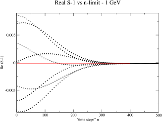
Figure 1: Real part of S compared to Kato Birman approximation as function of $n$.

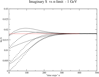
Figure 2: Imaginary part of S compared to Kato Birman approximation as function of $n$.

Table 1: Degree 300 polynomial compared to $e^{-inx}$, $n=220$

$x$	$\Delta\cos(nx)$	$\Delta\sin(nx)$
0	$4.44089\times 10^{-16}$	$8.32667\times 10^{-15}$
0.1	$2.35367\times 10^{-14}$	$1.46966\times 10^{-14}$
0.2	$5.55112\times 10^{-16}$	$3.6797\phantom{0}\times 10^{-14}$
0.3	$3.84137\times 10^{-14}$	$1.80689\times 10^{-14}$
0.4	$1.72085\times 10^{-14}$	$1.32672\times 10^{-14}$
0.5	$2.77556\times 10^{-15}$	$2.93793\times 10^{-14}$
0.6	$6.66134\times 10^{-16}$	$3.33344\times 10^{-14}$
0.7	$8.54872\times 10^{-15}$	$2.50355\times 10^{-14}$
0.8	$1.02141\times 10^{-14}$	$1.35447\times 10^{-14}$
0.9	$1.22125\times 10^{-15}$	$2.72282\times 10^{-14}$
1	$4.88498\times 10^{-15}$	$6.61415\times 10^{-14}$

Figure 3: Calculated compared to approximate calculations for the real part of transition matrix element for different energies.

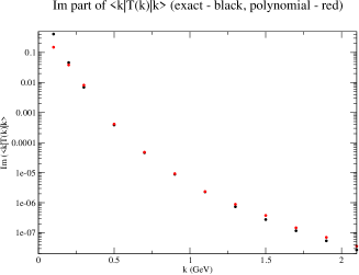
Figure 4: Calculated compared to approximate calculations for the real part of transition matrix element for different energies.

In this model sharp $T$ matrix elements can be calculated with an error of approximately 1% using wave packets whose momentum widths are about 1/10 of the cm momentum. Figures 1 and 2 show the convergence of the real and imaginary parts of the $S$ matrix evaluated in these wave packets as a function of $n$ in equation (39). Values of $n$ between 200-300 are adequate in this model. $\beta$ is a parameter that can be adjusted to improve the convergence. Polynomial approximations to $e^{2ine^{-\beta H}}$ are performed using Chebyshev expansions:

$$e^{inx}\approx{1\over 2}c_{0}T_{0}(x)+\sum_{k=1}^{N}c_{k}T_{k}(x)\qquad c_{j}={2\over N+1}\sum_{k=1}^{N}e^{in(\cos({2k-1\over N+1}{\pi\over 2}))}\cos(j{2k-1\over N+1}{\pi\over 2}).$$ (41)

Polynomials of degree approximately 300 agree with $e^{2ine^{-\beta H}}$ uniformly to better than 13 significant figures.

Typical results are shown in table 1. Figures 3 and 4 compare the exact value of the real and imaginary parts of the sharp momentum transition matrix to the calculated values for momenta up to 2 GeV. For most values of $k$ the exact and approximate values cannot be distinguished.

These results suggest that it may be feasible to use this method to formulate relativistic few-body models. The open problems that have not been addressed in this preliminary work involve finding model Green functions or generating functionals satisfying the required conditions. Reflection positivity appears to be a fairly restrictive condition that requires additional study. The toy model discussed above did not require solutions of the one-body problem. How approximate solutions of the one-body problem are affected by the other approximations also requires further study.

This work supported in part by the U.S. Department of Energy, under contract DE-FG02-86ER40286.

References

• (1) K. Osterwalder and R. Schrader, Commun. Math. Phys. 31, 83 (1973).
• (2) K. Osterwalder and R. Schrader, Commun. Math. Phys. 42, 281 (1975).
• (3) J. Fröhlich, Helv. Phys. Acta. 47, 265 (1974).
• (4) J. Glimm and A. Jaffe, Quantum Physics; A functional Integral Poinct of View (Springer-Verlag, 1981).
• (5) A. Klein and L. L., J. Functional Anal. 44, 121 (1981).
• (6) A. Klein and L. L., Comm. Math. Phys 87, 469 (1983).
• (7) J. Fröhlich, K. Osterwalder, and E. Seiler, Annals Math. 118, 461 (1983).
• (8) R. Haag, Phys. Rev. 112, 669 (1958).
• (9) D. Ruelle, Helv. Phys. Acta. 35, 147 (1962).
• (10) F. Coester, Helv. Phys. Acta. 38, 7 (1965).
• (11) M. Reed and B. Simon, Methods of Modern mathematical Physics, vol. III Scattering Theory (Academic Press, 1979).
• (12) H. Baumgärtel and M. Wollenberg, Mathematical Scattering Theory (Spinger-Verlag, Berlin, 1983).