Union Support Recovery in Multi-task Learning

Abstract

We sharply characterize the performance of different penalization schemes for the problem of selecting the relevant variables in the multi-task setting. Previous work focuses on the regression problem where conditions on the design matrix complicate the analysis. A clearer and simpler picture emerges by studying the Normal means model. This model, often used in the field of statistics, is a simplified model that provides a laboratory for studying complex procedures.

Keywords: high-dimensional inference, multi-task learning, sparsity, Normal means, minimax estimation

1 Introduction

We consider the problem of estimating a sparse, signal in the presence of noise. It has been empirically observed, on various data sets ranging from cognitive neuroscience Liu et al. (2009) to genome-wide association mapping studies Kim et al. (2009), that considering related estimation tasks jointly, improves estimation performance. Because of this, joint estimation from related tasks or multi-task learning has received much attention in the machine learning and statistics community (see for example Zhang, 2006; Negahban and Wainwright, 2009; Obozinski et al., 2010; Lounici et al., 2009; Liu et al., 2009; Lounici et al., 2010; Argyriou et al., 2008; Kim et al., 2009, and references therein). However, the theory behind multi-task learning is not yet settled.

An example of multi-task learning problem is the problem of estimating the coefficients of several multiple regression problems

$$\mathbf{y}_{j}=\mathbf{X}_{j}\bm{\beta}_{j}+\bm{\epsilon}_{j},\qquad j\in[k]$$ (1)

where $\mathbf{X}_{j}\in\mathbb{R}^{n\times p}$ is the design matrix, $\mathbf{y}_{j}\in\mathbb{R}^{n}$ is the vector of observations, $\bm{\epsilon}_{j}\in\mathbb{R}^{n}$ is the noise vector, $\bm{\beta}_{j}\in\mathbb{R}^{p}$ is the unknown vector of regression coefficients for the $j$-th task and $[n]=\{1,\ldots,n\}$.

When the number of variables $p$ is much larger than the sample size $n$, it is commonly assumed that the regression coefficients are jointly sparse, that is, there exists a small subset $S\subset[p]$, with $s:=|S|\ll n$, of the regression coefficients that are non-zero for all or most of the tasks.

The model in (1) under the joint sparsity assumption was analyzed in, for example, Obozinski et al. (2010), Lounici et al. (2009), Negahban and Wainwright (2009), Lounici et al. (2010) and Kolar and Xing (2010). Obozinski et al. (2010) propose to minimize the penalized least squares objective with the mixed $(2,1)$-norm of the coefficients as the penalty term. The authors focus on consistent estimation of the support set $S$, albeit under the assumption that the number of tasks $k$ is fixed. Negahban and Wainwright (2009) use the mixed $(\infty,1)$-norm of the coefficients as the penalty term instead and focus on the exact recovery of the non-zero pattern of the regression coefficients, rather than the support set $S$. For a rather limited case of $k=2$, the authors show that when the regression do not share a common support, it may be harmful to consider the regression problems jointly using the mixed $(\infty,1)$-norm penalty. Kolar and Xing (2010) address the feature selection properties of the simultaneous greedy forward selection, however, it is not clear what the benefits are compared to the ordinary forward selection done on each task separately. In Lounici et al. (2009) and Lounici et al. (2010), the focus is shifted from the consistent selection to benefits of the joint estimation for the prediction accuracy and consistent estimation. The number of tasks $k$ is allowed to increase with the sample size, however, it is assumed that all tasks share the same features, that is, a relevant coefficient is non-zero for all tasks.

Despite these previous investigations, the theory is far from settled. A simple clear picture of when sharing between tasks actually improves performance has not emerged. In particular, to the best of our knowledge, there has been no previous work that sharply characterizes the performance of different penalization schemes on the problem of selecting the relevant variables in the multi-task setting.

In this paper we study multi-task learning in the context of the many Normal means model. This is a simplified model that is often useful for studying the theoretical properties of procedures. The use of the many Normal means model is fairly common in statistics but appears to be less common in machine learning.

1.1 The Normal Means Model

The simplest Normal means model has the form

$$Y_{i}=\mu_{i}+\sigma\epsilon_{i},\ \ \ \ \ i=1,\ldots,p$$ (2)

where $\mu_{1},\ldots,\mu_{p}$ are unknown parameters and $\epsilon_{1},\ldots,\epsilon_{p}$ are independent, identically distributed Normal random variables with mean 0 and variance 1. There are a variety of results (Brown and Low (1996), Nussbaum (1996)) that show that many learning problems can be converted into a Normal means problem. This implies that results obtained in the Normal means setting can be transferred to many other settings. As a simple example, consider the nonparametric regression model $Z_{i}=m(i/n)+\delta_{i}$ where $m$ is a smooth function on $[0,1]$ and $\delta_{i}\sim N(0,1)$. Let $\phi_{1},\phi_{2},\ldots,$ be an orthonormal basis on [0,1] and write $m(x)=\sum_{j=1}^{\infty}\mu_{j}\phi_{j}(x)$ where $\mu_{j}=\int_{0}^{1}m(x)\phi_{j}(x)dx$. To estimate the regression function $m$ we need only estimate $\mu_{1},\mu_{2},\ldots,$. Let $Y_{j}=n^{-1}\sum_{i=1}^{n}Z_{i}\,\phi_{j}(i/n)$. Then $Y_{j}\approx N(\mu_{j},\sigma^{2})$ where $\sigma^{2}=1/n$. This has the form of (2) with $\sigma=1/\sqrt{n}$. Hence this regression problem can be converted into a Normal means model.

However, the most important aspect of the Normal means model is that it allows a clean setting for studying complex problems. In this paper, we consider the following Normal means model. Let

$$Y_{ij}=\left\{\begin{array}[]{cl}(1-\epsilon)\mathcal{N}(0,\sigma^{2})+\epsilon\mathcal{N}(\mu_{ij},\sigma^{2})&\quad j\in[k],\quad i\in S\\ N(0,\sigma^{2})&\quad j\in[k],\quad i\in S^{c}\\ \end{array}\right.$$ (3)

where $(\mu_{ij})_{i,j}$ are unknown real numbers, $\sigma=\sigma_{0}/\sqrt{n}$ is the variance with $\sigma_{0}>0$ known, $(Y_{ij})_{i,j}$ are random observations, $\epsilon\in[0,1]$ is the parameter that controls the sparsity of features across tasks and $S\subset[p]$ is the set of relevant features. Let $s=|S|$ denote the number of relevant features. Denote the matrix $M\in\mathbb{R}^{p\times k}$ of means

	Tasks
		1	2	$\ldots$	k
	1	$\mu_{11}$	$\mu_{12}$	$\ldots$	$\mu_{1k}$
	2	$\mu_{21}$	$\mu_{22}$	$\ldots$	$\mu_{2k}$
	$\vdots$	$\vdots$	$\vdots$	$\ddots$	$\vdots$
	p	$\mu_{p1}$	$\mu_{p2}$	$\ldots$	$\mu_{pk}$

and let $\bm{\theta}_{i}=(\mu_{ij})_{j\in[k]}$ denote the $i$-th row of the matrix $M$. The set $S^{c}=[p]\backslash S$ indexes the zero rows of the matrix $M$ and the associated observations are distributed according to the normal distribution with zero mean and variance $\sigma^{2}$. The rows indexed by $S$ are non-zero and the corresponding observation are coming from a mixture of two normal distributions. The parameter $\epsilon$ determines the proportion of observations coming from a normal distribution with non-zero mean. The reader should regard each column as one vector of parameters that we want to estimate. The question is whether sharing across columns improves the estimation performance.

It is known from the work on the Lasso that in regression problems, the design matrix needs to satisfy certain conditions in order for the Lasso to correctly identify the support $S$ (see van de Geer and Bühlmann, 2009, for an extensive discussion on the different conditions). These regularity conditions are essentially unavoidable. However, the Normal means model (3) allows us to analyze the estimation procedure in (5) and focus on the scaling of the important parameters $(n,k,p,s,\epsilon,\mu_{\min})$ for the success of the support recovery. Using the model (3) and the estimation procedure in (5), we are able to identify regimes in which estimating the support is more efficient using the ordinary Lasso than with the multi-task Lasso and vice versa. Our results suggest that multi-task Lasso does not outperform the ordinary Lasso when the features are not considerably shared across tasks and practitioners should be careful when applying the multi-task Lasso without knowledge of the task structure.

An alternative representation of the model is

$$Y_{ij}=\left\{\begin{array}[]{cl}\mathcal{N}(\xi_{ij}\mu_{ij},\sigma^{2})&\quad j\in[k],\quad i\in S\\ N(0,\sigma^{2})&\quad j\in[k],\quad i\in S^{c}\\ \end{array}\right.$$ (4)

where $\xi_{ij}$ is a Bernoulli random variable with success probability $\epsilon$. Throughout the paper, we will set $\epsilon=k^{-\beta}$ for some parameter $\beta\in[0,1)$. $\beta<1/2$ corresponds to dense rows and $\beta>1/2$ corresponds to sparse rows. Let $\mu_{\min}$ denote the absolute value of a smallest non-zero element of $M$, $\mu_{\min}=\min|\mu_{ij}|$.

Under the model (3), we analyze the penalized least squares procedures of the form

$$\widehat{\bm{\mu}}=\mathop{\mathrm{argmin}}_{\bm{\mu}\in\mathbb{R}^{p\times k}}\ \frac{1}{2}||\mathbf{Y}-\bm{\mu}||_{F}^{2}+{\rm pen}(\bm{\mu})$$ (5)

where $||A||_{F}=\sum_{jk}A_{jk}^{2}$ is the Frobenious norm, ${\rm pen}(\cdot)$ is a penalty function and $\bm{\mu}$ is a $p\times k$ matrix of means. We consider the following penalties

1. the $\ell_{1}$ penalty

   $${\rm pen}(\bm{\mu})=\lambda\sum_{i\in[p]}\sum_{j\in[k]}|\mu_{ij}|,$$

   which corresponds to the Lasso procedure applied on each task independently, and denote the resulting estimate as $\widehat{\bm{\mu}}^{\ell_{1}}$

2. the mixed $(2,1)$-norm penalty

   $${\rm pen}(\bm{\mu})=\lambda\sum_{i\in[p]}||\theta_{i}||_{2},$$

   which corresponds to the multi-task Lasso formulation in Obozinski et al. (2010) and Lounici et al. (2009), and denote the resulting estimate as $\widehat{\bm{\mu}}^{\ell_{1}/\ell_{2}}$

3. the mixed $(\infty,1)$-norm penalty

   $${\rm pen}(\bm{\mu})=\lambda\sum_{i\in[p]}||\theta_{i}||_{\infty},$$

   which correspond to the multi-task Lasso formulation in Negahban and Wainwright (2009), and denote the resulting estimate as $\widehat{\bm{\mu}}^{\ell_{1}/\ell_{2}}$.

For any solution $\widehat{\bm{\mu}}$ of (5), let $S(\widehat{\bm{\mu}})$ denote the set of estimated non-zero rows

$$S(\widehat{\bm{\mu}})=\{i\in[p]\ :\ ||\widehat{\bm{\theta}}_{i}||_{2}\neq 0\}.$$ (6)

We establish sufficient conditions under which $\mathbb{P}[S(\widehat{\bm{\mu}})\neq S]\leq\alpha$ for different methods. These results are complemented with necessary conditions for the recovery of the support set $S$.

1.2 Overview of the main results

The main contributions of the paper can be summarized as follows.

1. We establish a lower bound on the parameter $\mu_{\min}$ as a function of the parameters $(n,k,p,s,\beta)$. Our result can be interpreted as follows: for any estimation procedure there exists a model given by (3) with non-zero elements equal to $\mu_{\min}$ such that the estimation procedure will make an error when identifying the set $S$ with probability bounded away from zero.

2. We establish the sufficient conditions on the signal strength $\mu_{\min}$ for the Lasso and both variants of the group Lasso under which these procedures can correctly identify the set of non-zero rows $S$.

By comparing the lower bounds with the sufficient conditions, we are able to identify regimes in which each procedure is optimal for the problem of identifying the set of non-zero rows $S$. Furthermore, we point out that the usage of the popular group Lasso with the mixed $(\infty,1)$ norm can be disastrous when features are not perfectly shared among tasks. This is further demonstrated using through an empirical study.

1.3 Organization of the paper

The paper is organizes as follows. We start by analyzing the lower bound for any procedure for the problem of identifying the set of non-zero rows in $\S$2. In $\S$3 we provide sufficient conditions on the signal strength $\mu_{\min}$ for the Lasso and the group Lasso to be able to detect the set of non-zero rows $S$. In the following section, we propose an improved approach to the problem of estimating the set $S$. Results of a small empirical study are reported in $\S$5. We close the paper by a discussion of our findings.

2 Lower bound on the support recovery

In this section, we derive a lower bound for the problem of identifying the correct variables. In particular, we derive conditions on $(n,k,p,s,\epsilon,\mu_{\min})$ under which any method is going to make an error when estimating the correct variables. Intuitively, if $\mu_{\min}$ is very small, a non-zero row may be hard to distinguish from a zero row. Similarly, if $\epsilon$ is very small, many elements in a row will zero and, again, as a result it may be difficult to identify a non-zero row. Before, we give the main result of the section, we introduce the class of models that are going to be considered.

Let

$$\mathcal{F}[\mu]:=\{\bm{\theta}\in\mathbb{R}^{k}\ :\ \min_{j}|\theta_{j}|\geq\mu\}$$

denote the set of feasible non-zero rows. For each $j\in\{0,1,\ldots,k\}$, let $\mathcal{M}(j,k)$ be the class of all the subsets of $\{1,\ldots,k\}$ of cardinality $j$. Let

$$\mathbb{M}[\mu,s]=\left\{(\bm{\theta}_{1},\ldots,\bm{\theta}_{p})^{\prime}\in\mathbb{R}^{p\times k}\ :\ \omega\in\mathcal{M}(s,p),\ \bm{\theta}_{i}=\left\{\begin{array}[]{cc}\in\mathcal{F}[\mu]&\text{ if }i\in\omega\\ {\bf 0}&\text{ if }i\not\in\omega\end{array}\right.\right\}$$ (7)

be the class of all feasible matrix means. For a matrix $M\in\mathbb{M}[\mu,s]$, let $\mathbb{P}_{M}$ denote the joint law of $\{Y_{ij}\}_{i\in[p],j\in[k]}$. Since $\mathbb{P}_{M}$ is a product measure, we can write $\mathbb{P}_{M}=\otimes_{i\in[p]}\mathbb{P}_{\bm{\theta}_{i}}$. For a non-zero row $\bm{\theta}_{i}$, we set

$$\mathbb{P}_{\bm{\theta}_{i}}(A)=\int\mathcal{N}(A;\widehat{\bm{\theta}},\sigma^{2}\mathbf{I}_{k})d\nu(\widehat{\bm{\theta}}),\qquad A\in\mathcal{B}(\mathbb{R}^{k}),$$

where $\nu$ is the distribution of the random variable $\sum_{j\in k}\mu_{ij}\xi_{j}e_{j}$ with $\xi_{j}\sim{\rm Bernoulli}(k^{-\beta})$ and $\{e_{j}\}_{j\in[k]}$ denoting the canonical basis of $\mathbb{R}^{k}$. For a zero row $\bm{\theta}_{i}={\bf 0}$, we set

$$\mathbb{P}_{{\bf 0}}(A)=\mathcal{N}(A;{\bf 0},\sigma^{2}\mathbf{I}_{k}),\qquad A\in\mathcal{B}(\mathbb{R}^{k}).$$

With this notation, we have the following results.

Theorem 1

Let

$$\mu_{\min}^{2}=\mu_{\min}^{2}(n,k,p,s,\epsilon,\beta)=\ln\Big{(}1+u+\sqrt{2u+u^{2}}\Big{)}\sigma^{2}$$ (8)

where

$$u=\frac{\ln\Big{(}1+\frac{\alpha^{2}(p-s+1)}{2}\Big{)}}{2k^{1-2\beta}}.$$

If $\alpha\in(0,\frac{1}{2})$ and $k^{-\beta}u<1$, then for all $\mu\leq\mu_{\min}$,

$$\inf_{\widehat{\mu}}\sup_{M\in\mathbb{M}[\mu,s]}\mathbb{P}_{M}[S(\widehat{\mu})\neq S(M)]\geq\frac{1}{2}(1-\alpha)$$ (9)

where $\mathbb{M}[\mu,s]$ is given by (7).

The result can be interpreted in words in the following way: whatever the estimation procedure $\widehat{\mu}$, there exists some matrix $M\in\mathbb{M}[\mu_{\min},s]$ such that the probability of incorrectly identifying the support $S(M)$ is bounded away from zero. In the next section, we will see that some estimation procedures achieve the lower bound given in Theorem 1.

3 Upper bounds on the support recovery

In this section, we present sufficient conditions on $(n,p,k,\epsilon,\mu_{\min})$ for different estimation procedures, so that

$$\mathbb{P}[S(\widehat{\bm{\mu}})\neq S]\leq\alpha.$$

Let $\alpha^{\prime},\delta^{\prime}>0$ be two parameters such that $\alpha^{\prime}+\delta^{\prime}=\alpha$. The parameter $\alpha^{\prime}$ controls the probability of making a type one error

$$\mathbb{P}[\exists i\in[p]\ :\ i\in S(\widehat{\bm{\mu}})\text{ and }i\not\in S]\leq\alpha^{\prime},$$

that is, the parameter $\alpha^{\prime}$ upper bounds the probability that there is a zero row of the matrix $M$ that is estimated as a non-zero row. Likewise, the parameter $\delta^{\prime}$ controls the probability of making a type two error

$$\mathbb{P}[\exists i\in[p]\ :\ i\not\in S(\widehat{\bm{\mu}})\text{ and }i\in S]\leq\delta^{\prime},$$

that is, the parameter $\delta^{\prime}$ upper bounds the probability that there is a non-zero row of the matrix $M$ that is estimated as a zero row.

The control of the type one and type two errors is established through the tuning parameter $\lambda$. It can be seen that if the parameter $\lambda$ is chosen such that, for all $i\in S$, it holds that $\mathbb{P}[i\not\in S(\widehat{\bm{\mu}})]\leq\delta^{\prime}/s$ and, for all $i\in S^{c}$, it hold that $\mathbb{P}[i\in S(\widehat{\bm{\mu}})]\leq\alpha^{\prime}/(p-s)$, then using the union bound we have that $\mathbb{P}[S(\widehat{\bm{\mu}})\neq S]\leq\alpha$. In the following subsections, we will use the outlined strategy to choose $\lambda$ for different estimation procedures.

3.1 Upper bounds for the Lasso

Recall that the Lasso estimator is given as

$$\widehat{\bm{\mu}}^{\ell_{1}}=\mathop{\mathrm{argmin}}_{\bm{\mu}\in\mathbb{R}^{p\times k}}\ \frac{1}{2}||\mathbf{Y}-\bm{\mu}||_{F}^{2}+\lambda||\bm{\mu}||_{1}.$$ (10)

It is easy to see that the solution of the above estimation problem is given as the following soft-thresholding operation

$$\widehat{\mu}_{ij}^{\ell_{1}}=\left(1-\frac{\lambda}{|Y_{ij}|}\right)_{+}Y_{ij},$$ (11)

where $(x)_{+}:=\max(0,x)$. From (11), it is obvious that $i\in S(\widehat{\bm{\mu}}^{\ell_{1}})$ if and only if the maximum statistics, defined as

$$M_{k}(i)=\max_{j}|Y_{ij}|,$$

satisfies $M_{k}(i)\geq\lambda$. Therefore it is crucial to find the critical value of the parameter $\lambda$ such that

$$\left\{\begin{array}[]{cccl}\mathbb{P}[M_{k}(i)<\lambda]&<&\delta^{\prime}/s&\quad i\in S\\ \mathbb{P}[M_{k}(i)>\lambda]&<&\alpha^{\prime}/(p-s)&\quad i\in S^{c}.\\ \end{array}\right.$$

We start by controlling the type one error. For $i\in S^{c}$ it holds that

$$\mathbb{P}[M_{k}(i)\geq\lambda]\leq k\mathbb{P}[|\mathcal{N}(0,\sigma^{2})|\geq\lambda]\leq\frac{2k\sigma}{\sqrt{2\pi}\lambda}\exp\big{(}-\frac{\lambda^{2}}{2\sigma^{2}}\big{)}$$ (12)

using lemma 7. Setting the right hand side to $\alpha^{\prime}/(p-s)$ in the above display, we obtain that $\lambda$ can be set as

$$\lambda=\sigma\sqrt{2\ln\frac{2k(p-s)}{\sqrt{2\pi}\alpha^{\prime}}}$$ (13)

and (12) holds as soon as $2\ln\frac{2k(p-s)}{\sqrt{2\pi}\alpha^{\prime}}\geq 1$. Next, we deal with the type two error. Let

$$\pi_{k}=\mathbb{P}[|(1-\epsilon)\mathcal{N}(0,\sigma^{2})+\epsilon\mathcal{N}(\mu_{\min},\sigma^{2})|>\lambda].$$ (14)

Then for $i\in S$, $\mathbb{P}[M_{k}(i)<\lambda]\leq\mathbb{P}[{\rm Bin}(k,\pi_{k})=0]$, where ${\rm Bin}(k,\pi_{k})$ denotes the binomial random variable with parameters $(k,\pi_{k})$. Control of the type two error is going to be established through careful analysis of $\pi_{k}$ for various regimes of problem parameters.

Theorem 2

Let $\lambda$ be defined by (13). Suppose $\mu_{\min}$ satisfies one of the following two cases:

1. $\mu_{\min}=\sigma\sqrt{2r\ln k}$ where

   $$r>\bigg{(}\sqrt{1+C_{k,p,s}}-\sqrt{1-\beta}\bigg{)}^{2}$$

   with

   $$C_{k,p,s}=\frac{\ln\frac{2(p-s)}{\sqrt{2\pi}\alpha^{\prime}}}{\ln k}$$

   and $\lim_{n\rightarrow\infty}C_{k,p,s}\in[0,\infty)$;

2. $\mu_{\min}\geq\lambda$ when

   $$\lim_{n\rightarrow\infty}\frac{\ln k}{\ln(p-s)}=0$$

   and $k^{1-\beta}/2\geq\ln(s/\delta^{\prime})$.

Then

$$\mathbb{P}[S(\widehat{\bm{\mu}}^{\ell_{1}})\neq S]\leq\alpha.$$

The proof is given in $\S$7.2.

Now we can compare the lower bound on $\mu_{\min}^{2}$ from Theorem 1 and the upper bound from Theorem 2. Without loss of generality we assume that $\sigma=1$. We have that when $\beta<1/2$ the lower bound is of the order $\mathcal{O}\left(\ln\left(k^{\beta-1/2}\ln(p-s)\right)\right)$ and the upper bound is of the order $\ln(k(p-s))$. Ignoring the logarithmic terms in $p$ and $s$, we have that the lower bound is of the order $\widetilde{\mathcal{O}}(k^{\beta-1/2})$ and the upper bound is of the order $\widetilde{\mathcal{O}}(\ln k)$, which implies that the Lasso does not achieve the lower bound when the non-zero rows are dense. When the non-zero rows are sparse, $\beta>1/2$, we have that both the lower and upper bound are of the order $\widetilde{\mathcal{O}}(\ln k)$ (ignoring the terms depending on $p$ and $s$).

3.2 Upper bounds for the group Lasso

Recall that the group Lasso estimator is given as

$$\widehat{\bm{\mu}}^{\ell_{1}/\ell_{2}}=\mathop{\mathrm{argmin}}_{\bm{\mu}\in\mathbb{R}^{p\times k}}\ \frac{1}{2}||\mathbf{Y}-\bm{\mu}||_{F}^{2}+\lambda\sum_{i\in[p]}||\bm{\theta}_{i}||_{2},$$ (15)

where $\bm{\theta}_{i}=(\mu_{ij})_{j\in[k]}$. The group Lasso estimator can be obtained in a closed form as a result of the following thresholding operation (see, for example, Friedman et al., 2010)

$$\widehat{\bm{\theta}}_{i}^{\ell_{1}/\ell_{2}}=\left(1-\frac{\lambda}{||Y_{i\cdot}||{2}}\right)_{+}Y_{i\cdot}$$ (16)

where $Y_{i\cdot}$ is the $i^{\rm th}$ row of the data. From (16), it is obvious that $i\in S(\widehat{\bm{\mu}}^{\ell_{1}/\ell_{2}})$ if and only if the statistic defined as

$$S_{k}(i)=\sum_{j}Y_{ij}^{2},$$

satisfies $S_{k}(i)\geq\lambda$. The choice of $\lambda$ is crucial for the control of type one and type two errors. We use the following result, which directly follows from Theorem 2 in Baraud (2002).

Lemma 3

Let $\{Y_{i}=f_{i}+\sigma\xi_{i}\}_{i\in[n]}$ be a sequence of independent observations, where $f=\{f_{i}\}_{i\in[n]}$ is a sequence of numbers, $\xi_{i}\stackrel{{\scriptstyle{iid}}}{{\sim}}\mathcal{N}(0,1)$ and $\sigma$ is a known positive constant. Suppose that $t_{n,\alpha}\in\mathbb{R}$ satisfies $\mathbb{P}[\chi^{2}_{n}>t_{n,\alpha}]\leq\alpha$. Let

$$\phi_{\alpha}=I\{\sum_{i\in[n]}Y_{i}^{2}\geq t_{n,\alpha}\sigma^{2}\}$$

be a test for $f=0$ versus $f\neq 0$. Then the test $\phi_{\alpha}$ satisfies

$$\mathbb{P}[\phi_{\alpha}=1]\leq\alpha$$

when $f=0$ and

$$\mathbb{P}[\phi_{\alpha}=0]\leq\delta$$

for all $f$ such that

$$||f||_{2}^{2}\geq 2(\sqrt{5}+4)\sigma^{2}\ln\left(\frac{2e}{\alpha\delta}\right)\sqrt{n}.$$

Proof  Follows immediately from Theorem 2 in Baraud (2002).  
It follows directly from lemma 3 that setting

$$\lambda=t_{n,\alpha^{\prime}/(p-s)}\sigma^{2}$$ (17)

will control the probability of type one error at the desired level, that is,

$$\mathbb{P}[S_{k}(i)\geq\lambda]\leq\alpha^{\prime}/(p-s),\qquad\forall i\in S^{c}.$$

The following theorem gives us the control of the type two error.

Theorem 4

Let $\lambda=t_{n,\alpha^{\prime}/(p-s)}\sigma^{2}$. Then

$$\mathbb{P}[S(\widehat{\bm{\mu}}^{\ell_{1}/\ell_{2}})\neq S]\leq\alpha$$

if

$$\mu_{\min}\geq\sigma\sqrt{2(\sqrt{5}+4)}\sqrt{\frac{k^{-1/2+\beta}}{1-c}}\sqrt{\ln\frac{2e(2s-\delta^{\prime})(p-s)}{\alpha^{\prime}\delta^{\prime}}}$$

where $c=\sqrt{2\ln(2s/\delta^{\prime})/k^{1-\beta}}$.

The proof is given in $\S$7.3.

Using Theorem 1 and Theorem 4 we can compare the lower bound on $\mu_{\min}^{2}$ and the upper bound. Without loss of generality we assume that $\sigma=1$. When each non-zero row is dense, that is, when $\beta<1/2$, we have that both lower and upper bounds are of the order $\widetilde{\mathcal{O}}(k^{\beta-1/2})$ (ignoring the logarithmic terms in $p$ and $s$). This suggest that the group Lasso performs better than the Lasso for the case where there is a lot of feature sharing between different tasks. Recall from previous section that the Lasso in this setting does not have the optimal dependence on $k$. However, when $\beta>1/2$, that is, in the sparse non-zero row regime, we see that the lower bound is of the order $\widetilde{\mathcal{O}}(\ln(k))$ whereas the upper bound is of the order $\widetilde{\mathcal{O}}(k^{\beta-1/2})$. This implies that the group Lasso does not have optimal dependence on $k$ in the sparse non-zero row setting.

3.3 Upper bounds for the group Lasso with the mixed $(\infty,1)$ norm

In this section, we analyze the group Lasso estimator with the mixed $(\infty,1)$ norm, defined as

$$\widehat{\bm{\mu}}^{\ell_{1}/\ell_{\infty}}=\mathop{\mathrm{argmin}}_{\bm{\mu}\in\mathbb{R}^{p\times k}}\ \frac{1}{2}||\mathbf{Y}-\bm{\mu}||_{F}^{2}+\lambda\sum_{i\in[p]}||\bm{\theta}_{i}||_{\infty},$$ (18)

where $\bm{\theta}_{i}=(\mu_{ij})_{j\in[k]}$. The closed form solution for $\widehat{\bm{\mu}}^{\ell_{1}/\ell_{\infty}}$ can be obtained (see Liu et al., 2009), however, we are only going to use the following lemma.

Lemma 5

(Liu et al., 2009) $\widehat{\bm{\theta}}_{i}^{\ell_{1}/\ell_{\infty}}={\bf 0}$ if and only if $\sum_{j}|Y_{ij}|\leq\lambda$.

Proof  See the proof of Proposition 5 in Liu et al. (2009).  
Suppose that the penalty parameter $\lambda$ is set as

$$\lambda=k\sigma\sqrt{2\ln\frac{k(p-s)}{\alpha^{\prime}}}.$$ (19)

Then it follows directly from lemma 7 that

$$\mathbb{P}[\sum_{j}|Y_{ij}|\geq\lambda]\leq k\max_{j}\mathbb{P}[|Y_{ij}|\geq\lambda/k]\leq\alpha^{\prime}/(p-s),\qquad\forall i\in S^{c},$$

which implies that the probability of the type one error is controlled at the desired level.

Theorem 6

Let the penalty parameter $\lambda$ be defined by (19). Then

$$\mathbb{P}[S(\widehat{\bm{\mu}}^{\ell_{1}/\ell_{\infty}})\neq S]\leq\alpha$$

if

$$\mu_{\min}\ \geq\ \frac{1+\tau}{1-c}k^{-1+\beta}\lambda$$

where $c=\sqrt{2\ln(2s/\delta^{\prime})/k^{1-\beta}}$ and $\tau=\sigma\sqrt{2k\ln\frac{2s-\delta^{\prime}}{\delta^{\prime}}}/\lambda$.

The proof is given in $\S$7.4.

Comparing upper bounds for the Lasso and the group Lasso with the mixed $(2,1)$ norm with the result of Theorem 6, we can see that both the Lasso and the group Lasso have better dependence on $k$ than the group Lasso with the mixed $(\infty,1)$ norm. The difference becomes more pronounced as $\beta$ increases. This suggest that we should be very cautious when using the group Lasso with the mixed $(\infty,1)$ norm, since as soon as the tasks do not share exactly the same features, the other two procedures have much better performance on identifying the set of non-zero rows.

4 Improved estimation procedure

We have observed in the last section that the Lasso procedure performs better than the group Lasso when each non-zero row is sparse, while the group Lasso (with the mixed $(2,1)$ norm) performs better when each non-zero row is dense. Since in many practical situations one does not how much overlap there is between different tasks, it would be useful to combine the Lasso and the group Lasso in order to improve the performance. This can be simply done by estimating $S(\widehat{\bm{\mu}}^{\ell_{1}})$ using (10) and $S(\widehat{\bm{\mu}}^{\ell_{1}/\ell_{2}})$ using (15) separately. Finally, we can combine these estimates by taking their union $\widehat{S}=S(\widehat{\bm{\mu}}^{\ell_{1}})\cup S(\widehat{\bm{\mu}}^{\ell_{1}/\ell_{2}})$. The outlined approach has the advantage that one does not need to know in advance which estimation procedure to use. From the theoretical analysis of the Lasso and the group Lasso, we can see that controlling the error of omitting a non-zero row is more difficult that controlling the probability of falsely including a zero row. Therefore, combining the Lasso and the group Lasso estimate can be seen as a way to increase the power to detect the non-zero rows.

5 Simulation results

We conduct a small-scale empirical study of the performance of the Lasso and the group Lasso (both with the mixed $(2,1)$ norm and with the mixed $(\infty,1)$ norm). Our empirical study shows that the theoretical findings of $\S$3 describe sharply the behavior of procedures even for small sample studies. In particular, we demonstrate that as the minimum signal level $\mu_{\min}$ varies in the model (3), our theory sharply determines points at which probability of identifying non-zero rows of matrix $M$ successfully transitions from $0$ to $1$ for different procedures.

The simulation procedure can be described as follows. Without loss of generality we let $S=[s]$ and draw the samples $\{Y_{ij}\}_{i\in[p],j\in[k]}$ according to the model in (3). The total number of rows $p$ is varied in $\{128,256,512,1024\}$ and the number of columns is set to $k=\lfloor p\log_{2}(p)\rfloor$. The sparsity of each non-zero row is controlled by changing the parameter $\beta$ in $\{0,0.25,0.5,0.75\}$ and setting $\epsilon=k^{-\beta}$. The number of non-zero rows is set to $s=\lfloor\log_{2}(p)\rfloor$, the sample size is set to $n=0.1p$ and $\sigma_{0}=1$. The parameters $\alpha^{\prime}$ and $\delta^{\prime}$ are both set to $0.01$. For each setting of the parameters, we report our results averaged over 1000 simulation runs. Simulations with other choices of parameters $n,s$ and $k$ have been tried out, but the results were qualitatively similar and, hence, we do not report them here.

5.1 Lasso

We investigate the performance on the Lasso for the purpose of estimating the set of non-zero rows, $S$. Figure 1 plots the probability of success as a function of the signal strength. On the same figure we plot the probability of success for the group Lasso with both $(2,1)$ and $(\infty,1)$-mixed norms. Using theorem 2, we set

$$\mu_{\rm lasso}=\sqrt{2(r+0.001)\ln k}$$ (20)

where $r$ is defined in theorem 2. Next, we generate data according to (3) with all elements $\{\mu_{ij}\}$ set to $\mu=\rho\mu_{\rm lasso}$, where $\rho\in[0.05,2]$. The penalty parameter $\lambda$ is chosen as in (13). Figure 1 plots probability of success as a function of the parameter $\rho$, which controls the signal strength. This probability transitions very sharply from 0 to 1. A rectangle on a horizontal line represents points at which the probability $\mathbb{P}[\widehat{S}=S]$ is between $0.05$ and $0.95$. From each subfigure in Figure 1, we can observe that the probability of success for the Lasso transitions from $0$ to $1$ for the same value of the parameter $\rho$ for different values of $p$, which indicated that, except for constants, our theory correctly characterizes the scaling of $\mu_{\min}$. In addition, we can see that the Lasso outperforms the group Lasso (with $(2,1)$-mixed norm) when each non-zero row is very sparse (the parameter $\beta$ is close to one).

Probability of successful support recovery: Lasso

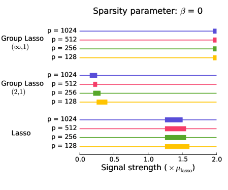
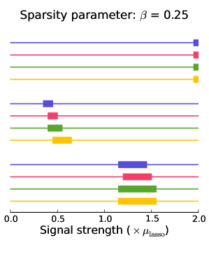
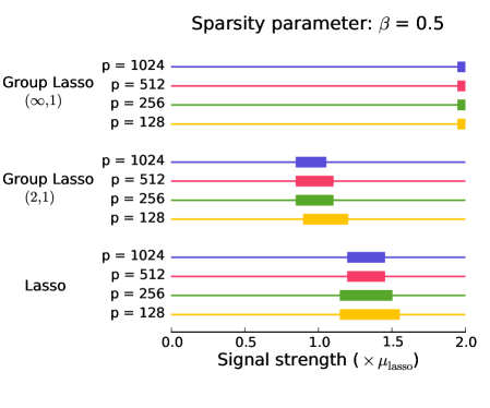
Figure 1: The probability of success for the Lasso for the problem of estimating $S$ plotted against the signal strength, which is varied as a multiple of $\mu_{\rm lasso}$ defined in (20). A rectangle on each horizontal line represents points at which the probability $\mathbb{P}[\widehat{S}=S]$ is between $0.05$ and $0.95$. Different subplots represent the probability of success as the sparsity parameter $\beta$ changes.

5.2 Group Lasso

Next, we focus on the empirical performance of the group Lasso with the mixed $(2,1)$ norm. Figure 2 plots the probability of success as a function of the signal strength. Using theorem 4, we set

$$\mu_{\rm group}=\sigma\sqrt{2(\sqrt{5}+4)}\sqrt{\frac{k^{-1/2+\beta}}{1-c}}\sqrt{\ln\frac{(2s-\delta^{\prime})(p-s)}{\alpha^{\prime}\delta^{\prime}}}$$ (21)

where $c$ is defined in theorem 4. Next, we generate data according to (3) with all elements $\{\mu_{ij}\}$ set to $\mu=\rho\mu_{\rm group}$, where $\rho\in[0.05,2]$. The penalty parameter $\lambda$ is given by (17). Figure 2 plots probability of success as a function of the parameter $\rho$, which controls the signal strength. A rectangle on a horizontal line represents points at which the probability $\mathbb{P}[\widehat{S}=S]$ is between $0.05$ and $0.95$. From each subfigure in Figure 2, we can observe that the probability of success for the group Lasso transitions from $0$ to $1$ for the same value of the parameter $\rho$ for different values of $p$, which indicated that, except for constants, our theory correctly characterizes the scaling of $\mu_{\min}$. We observe also that the group Lasso outperforms the Lasso when each non-zero row is not too sparse, that is, when there is a considerable overlap of features between different tasks.

Probability of successful support recovery: group Lasso

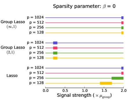
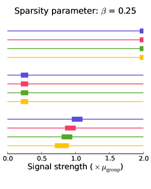
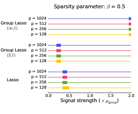
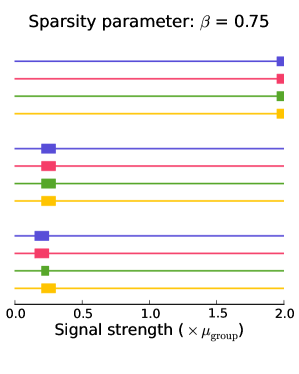
Figure 2: The probability of success for the group Lasso for the problem of estimating $S$ plotted against the signal strength, which is varied as a multiple of $\mu_{\rm group}$ defined in (21). A rectangle on each horizontal line represents points at which the probability $\mathbb{P}[\widehat{S}=S]$ is between $0.05$ and $0.95$. Different subplots represent the probability of success as the sparsity parameter $\beta$ changes.

5.3 Group Lasso with the mixed $(\infty,1)$ norm

Next, we focus on the empirical performance of the group Lasso with the mixed $(\infty,1)$ norm. Figure 3 plots the probability of success as a function of the signal strength. Using theorem 6, we set

$$\mu_{\rm infty}=\frac{1+\tau}{1-c}k^{-1+\beta}\lambda$$ (22)

where $\tau$ and $c$ are defined in theorem 6 and $\lambda$ is given by (19). Next, we generate data according to (3) with all elements $\{\mu_{ij}\}$ set to $\mu=\rho\mu_{\rm infty}$, where $\rho\in[0.05,2]$. Figure 3 plots probability of success as a function of the parameter $\rho$, which controls the signal strength. A rectangle on a horizontal line represents points at which the probability $\mathbb{P}[\widehat{S}=S]$ is between $0.05$ and $0.95$. From each subfigure in Figure 3, we can observe that the probability of success for the group Lasso transitions from $0$ to $1$ for the same value of the parameter $\rho$ for different values of $p$, which indicated that, except for constants, our theory correctly characterizes the scaling of $\mu_{\min}$. We also observe that the group Lasso with the mixed $(\infty,1)$ norm never outperforms the Lasso or the group Lasso with the mixed $(2,1)$ norm.

Probability of successful support recovery: group Lasso with the mixed $(\infty,1)$ norm

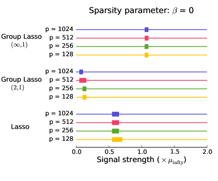
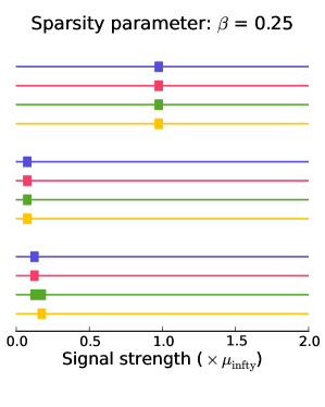
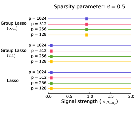
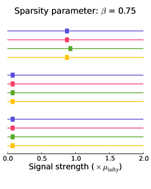
Figure 3: The probability of success for the group Lasso with mixed $(\infty,1)$ norm for the problem of estimating $S$ plotted against the signal strength, which is varied as a multiple of $\mu_{\rm infty}$ defined in (22). A rectangle on each horizontal line represents points at which the probability $\mathbb{P}[\widehat{S}=S]$ is between $0.05$ and $0.95$. Different subplots represent the probability of success as the sparsity parameter $\beta$ changes.

6 Discussion

We have studied the benefits of task sharing in sparse problems. Under many scenarios, the group lasso outperforms the lasso. The $\ell_{1}/\ell_{2}$ penalty seems to be a much better choice for the group lasso than the $\ell_{1}/\ell_{\infty}$. However, as pointed out to us by Han Liu, for screening, where false discoveries are less important than accurate recovery, it is possible that the $\ell_{1}/\ell_{\infty}$ penalty could be useful.

We focused on the Normal means model. While this model is obviously a simplified model, it is extremely useful for theoretical study. The Normal means model is commonly used in Statistics and we hope that this paper encourages researchers in machine learning to consider wider use of this model as well.

7 Proofs

This section collects technical proofs of the results presented in the paper. Throughout the section we use $c_{1},c_{2},\ldots$ to denote positive constants whose value may change from line to line.

7.1 Proof of Theorem 1

Without loss of generality, we may assume $\sigma=1$. Let $\phi(u)$ be the density of $\mathcal{N}(0,1)$ and define $\mathbb{P}_{{\bf 0}}$ and $\mathbb{P}_{{\bf 1}}$ to be two probability measures on $\mathbb{R}^{k}$ with the densities with respect to the Lebesgue measure given as

$$f_{0}(a_{1},\ldots,a_{k})=\prod_{j\in[k]}\phi(a_{j})$$ (23)

and

$$f_{1}(a_{1},\ldots,a_{k})=\mathbb{E}_{Z}\mathbb{E}_{m}\mathbb{E}_{\xi}\prod_{j\in m}\phi(a_{j}-\xi_{j}\mu_{\min})\prod_{j\not\in m}\phi(a_{j})$$ (24)

where $Z\sim{\rm Bin}(k,k^{-\beta})$, $m$ is a random variable uniformly distributed over $\mathcal{M}(Z,k)$ and $\{\xi_{j}\}_{j\in[k]}$ is a sequence of Rademacher random variables, independent of $Z$ and $m$. A Rademacher random variable takes values $\pm 1$ with probability $\frac{1}{2}$.

To simplify the discussion, suppose that $p-s+1$ is divisible by 2. Let $T=(p-s+1)/2$. Using $\mathbb{P}_{{\bf 0}}$ and $\mathbb{P}_{{\bf 1}}$, we construct the following three measures,

$$\widetilde{\mathbb{Q}}=\mathbb{P}_{{\bf 1}}^{s-1}\otimes\mathbb{P}_{{\bf 0}}^{p-s+1},$$

$$\mathbb{Q}_{0}=\frac{1}{T}\sum_{{j\in\{s,\ldots,p\}}\atop{j\text{ odd}}}\mathbb{P}_{{\bf 1}}^{s-1}\otimes\mathbb{P}_{{\bf 0}}^{j-s}\otimes\mathbb{P}_{{\bf 1}}\otimes\mathbb{P}_{{\bf 0}}^{p-j}$$

and

$$\mathbb{Q}_{1}=\frac{1}{T}\sum_{{j\in\{s,\ldots,p\}}\atop{j\text{ even}}}\mathbb{P}_{{\bf 1}}^{s-1}\otimes\mathbb{P}_{{\bf 0}}^{j-s}\otimes\mathbb{P}_{{\bf 1}}\otimes\mathbb{P}_{{\bf 0}}^{p-j}.$$

It holds that

$$\inf_{\widehat{\mu}}\sup_{M\in\mathbb{M}}\mathbb{P}_{M}[S(M)\neq S(\widehat{\mu})] \geq\inf_{\Psi}\max\ \Big{(}\mathbb{Q}_{0}(\Psi=1),\mathbb{Q}_{1}(\Psi=0)\Big{)}$$ (25)

$$\geq\frac{1}{2}-\frac{1}{2}||\mathbb{Q}_{0}-\mathbb{Q}_{1}||_{1},$$

where the infimum is taken over all tests $\Psi$ taking values in $\{0,1\}$ and $||\cdot||_{1}$ is the total variation distance between probability measures. For a readable introduction on lower bounds on the minimax probability of error, see Section 2 in Tsybakov (2009). In particular, our approach is related to the one described in Section 2.7.4. We proceed by upper bounding the total variation distance between $\mathbb{Q}_{0}$ and $\mathbb{Q}_{1}$. Let $g=d\mathbb{P}_{{\bf 1}}/d\mathbb{P}_{{\bf 0}}$ and let $u_{i}\in\mathbb{R}^{k}$ for each $i\in[p]$, then

$$\frac{d\mathbb{Q}_{0}}{d\widetilde{\mathbb{Q}}} (u_{1},\ldots,u_{p})$$

$$=\frac{1}{T}\sum_{{j\in\{s,\ldots,p\}}\atop{j\text{ even}}}\prod_{i\in\{1,\ldots,s-1\}}\frac{d\mathbb{P}_{{\bf 1}}}{d\mathbb{P}_{{\bf 1}}}(u_{i})\prod_{i\in\{s,\ldots,j-1\}}\frac{d\mathbb{P}_{{\bf 0}}}{d\mathbb{P}_{{\bf 0}}}(u_{i})\frac{d\mathbb{P}_{{\bf 1}}}{d\mathbb{P}_{{\bf 0}}}(u_{j})\prod_{i\in\{j+1,\ldots,p\}}\frac{d\mathbb{P}_{{\bf 0}}}{d\mathbb{P}_{{\bf 0}}}(u_{i})$$

$$=\frac{1}{T}\sum_{{j\in\{s,\ldots,p\}}\atop{j\text{ even}}}g(u_{j})$$

and, similarly, we can compute $d\mathbb{Q}_{1}/d\widetilde{\mathbb{Q}}$. The following holds

$$\| \mathbb{Q}_{0}-\mathbb{Q}_{1}\|_{1}^{2}$$ (26)

$$=\Bigg{(}\int\Big{|}\frac{1}{T}\big{(}\sum_{{j\in\{s,\ldots,p\}}\atop{j\text{ even}}}g(u_{j})-\sum_{{j\in\{s,\ldots,p\}}\atop{j\text{ odd}}}g(u_{j})\big{)}\Big{|}\prod_{i\in\{s,\ldots,p\}}d\mathbb{P}_{{\bf 0}}(u_{i})\Bigg{)}^{2}$$

$$\leq\frac{1}{T^{2}}\int\Big{(}\sum_{{j\in\{s,\ldots,p\}}\atop{j\text{ even}}}g(u_{j})-\sum_{{j\in\{s,\ldots,p\}}\atop{j\text{ odd}}}g(u_{j})\Big{)}^{2}\prod_{i\in\{s,\ldots,p\}}d\mathbb{P}_{{\bf 0}}(u_{i})$$

$$=\frac{2}{T}\big{(}\mathbb{P}_{{\bf 0}}(g^{2})-1\big{)},$$

where the last equality follows by observing that

$$\int\sum_{{j\in\{s,\ldots,p\}}\atop{j\text{ even}}}\sum_{{j^{\prime}\in\{s,\ldots,p\}}\atop{j^{\prime}\text{ even}}}g(u_{j})g(u_{j^{\prime}})\prod_{{i\in\{s,\ldots,p\}}\atop{i\text{ even}}}d\mathbb{P}_{{\bf 0}}(u_{i})=T\ \mathbb{P}_{{\bf 0}}(g^{2})+T^{2}-T$$

and

$$\int\sum_{{j\in\{s,\ldots,p\}}\atop{j\text{ even}}}\sum_{{j^{\prime}\in\{s,\ldots,p\}}\atop{j^{\prime}\text{ odd}}}g(u_{j})g(u_{j^{\prime}})\prod_{{i\in\{s,\ldots,p\}}}d\mathbb{P}_{{\bf 0}}(u_{i})=T^{2}.$$

Next, we proceed to upper bound $\mathbb{P}_{{\bf 0}}(g^{2})$, using some ideas presented in the proof of Theorem 1 in Baraud (2002). Recall definitions of $f_{0}$ and $f_{1}$ in (23) and (24) respectively. Then $g=d\mathbb{P}_{{\bf 1}}/d\mathbb{P}_{{\bf 0}}=f_{1}/f_{0}$ and we have

$$g(a_{1},\ldots,a_{k}) =\mathbb{E}_{Z}\mathbb{E}_{m}\mathbb{E}_{\xi}\bigg{[}\exp\Big{(}-\frac{Z\mu_{\min}^{2}}{2}+\mu_{\min}\sum_{j\in m}\xi_{j}a_{j}\Big{)}\bigg{]}$$

$$=\mathbb{E}_{Z}\bigg{[}\exp\Big{(}-\frac{Z\mu_{\min}^{2}}{2}\Big{)}\ \mathbb{E}_{m}\Big{[}\prod_{j\in m}\cosh(\mu_{\min}a_{j})\Big{]}\bigg{]}.$$

Furthermore, let $Z^{\prime}\sim{\rm Bin}(k,k^{-\beta})$ be independent of $Z$ and $m^{\prime}$ uniformly distributed over $\mathcal{M}(Z^{\prime},k)$. The following holds

$$\mathbb{P}_{{\bf 0}}(g^{2})$$

$$=\mathbb{P}_{{\bf 0}}\bigg{(}\mathbb{E}_{Z^{\prime},Z}\Big{[}\exp\Big{(}-\frac{(Z+Z^{\prime})\mu_{\min}^{2}}{2}\Big{)}\ \mathbb{E}_{m,m^{\prime}}\prod_{j\in m}\cosh(\mu_{\min}a_{j})\prod_{j\in m^{\prime}}\cosh(\mu_{\min}a_{j})\Big{]}\bigg{)}$$

$$=\mathbb{E}_{Z^{\prime},Z}\Big{[}\exp\Big{(}-\frac{(Z+Z^{\prime})\mu_{\min}^{2}}{2}\Big{)}$$

$$\qquad\qquad\qquad\mathbb{E}_{m,m^{\prime}}\Big{[}\prod_{j\in m\cap m^{\prime}}\int\cosh^{2}(\mu_{\min}a_{j})\phi(a_{j})da_{j}$$

$$\qquad\qquad\qquad\qquad\prod_{j\in m\triangle m^{\prime}}\int\cosh(\mu_{\min}a_{j})\phi(a_{j})da_{j}\Big{]}\Big{]},$$

where we use $m\triangle m^{\prime}$ to denote $(m\cup m^{\prime})\backslash(m\cap m^{\prime})$. By direct calculation, we have that

$$\int\cosh^{2}(\mu_{\min}a_{j})\phi(a_{j})da_{j}=\exp(\mu_{\min}^{2})\cosh(\mu_{\min}^{2})$$

and

$$\int\cosh(\mu_{\min}a_{j})\phi(a_{j})da_{j}=\exp(\mu_{\min}^{2}/2).$$

Since $\frac{1}{2}|m\triangle m^{\prime}|+|m\cap m^{\prime}|=(Z+Z^{\prime})/2$, we have that

$$\mathbb{P}_{{\bf 0}}(g^{2}) =\mathbb{E}_{Z,Z^{\prime}}\Big{[}E_{m,m^{\prime}}\Big{[}\big{(}\cosh(\mu_{\min}^{2})\big{)}^{|m\cap m^{\prime}|}\Big{]}\Big{]}$$

$$=\mathbb{E}_{Z,Z^{\prime}}\Big{[}\sum_{j=0}^{k}p_{j}\big{(}\cosh(\mu_{\min}^{2})\big{)}^{j}\Big{]}$$

$$=\mathbb{E}_{Z,Z^{\prime}}\Big{[}\mathbb{E}_{X}\Big{[}\cosh(\mu_{\min}^{2})^{X}\Big{]}\Big{]},$$

where

$$p_{j}=\left\{\begin{array}[]{cc}0&\text{if }j<Z+Z^{\prime}-k\text{ or }j>\min(Z,Z^{\prime})\\ \frac{{Z^{\prime}\choose j}{{k-Z^{\prime}}\choose{Z-j}}}{{k\choose Z}}&\text{otherwise}\end{array}\right.$$

and $P[X=j]=p_{j}$. Therefore, $X$ follows a hypergeometric distribution with parameters $k$, $Z$, $Z^{\prime}/k$. [The first parameter denotes the total number of stones in an urn, the second parameter denotes the number of stones we are going to sample without replacement from the urn and the last parameter denotes the fraction of white stones in the urn.] Then following (Aldous, 1985, p. 173; see also Baraud (2002)), we know that $X$ has the same distribution as the random variable $\mathbb{E}[\widetilde{X}|{\mathcal{T}}]$ where $\widetilde{X}$ is a binomial random variable with parameters $Z$ and $Z^{\prime}/k$, and ${\mathcal{T}}$ is a suitable $\sigma$-algebra. By convexity, it follows that

$$\mathbb{P}_{{\bf 0}}(g^{2}) \leq\mathbb{E}_{Z,Z^{\prime}}\Big{[}\mathbb{E}_{\widetilde{X}}\Big{[}\cosh(\mu_{\min}^{2})^{\widetilde{X}}\Big{]}\Big{]}$$

$$=\mathbb{E}_{Z,Z^{\prime}}\left[\exp\bigg{(}Z\ln\Big{(}1+\frac{Z^{\prime}}{k}\big{(}\cosh(\mu_{\min}^{2})-1\big{)}\Big{)}\bigg{)}\right]$$

$$=\mathbb{E}_{Z^{\prime}}\mathbb{E}_{Z}\left[\exp\bigg{(}Z\ln\Big{(}1+\frac{Z^{\prime}}{k}u\Big{)}\bigg{)}\right]$$

where $\mu_{\min}^{2}=\ln(1+u+\sqrt{2u+u^{2}})$ with

$$u=\frac{\ln\Big{(}1+\frac{\alpha^{2}T}{2}\Big{)}}{2k^{1-2\beta}}.$$

Continuing with our calculations, we have that

$$\mathbb{P}_{{\bf 0}}(g^{2}) =\mathbb{E}_{Z^{\prime}}\exp\Big{(}k\ln\big{(}1+k^{-(1+\beta)}uZ^{\prime}\big{)}\Big{)}$$ (27)

$$\leq\mathbb{E}_{Z^{\prime}}\exp\Big{(}k^{-\beta}uZ^{\prime}\Big{)}$$

$$=\exp\bigg{(}k\ln\Big{(}1+k^{-\beta}\big{(}\exp(k^{-\beta}u\big{)}-1)\Big{)}\bigg{)}$$

$$\leq\exp\Big{(}k^{1-\beta}\big{(}\exp\big{(}k^{-\beta}u\big{)}-1\big{)}\Big{)}$$

$$\leq\exp\Big{(}2k^{1-2\beta}u\Big{)}$$

$$=1+\frac{\alpha^{2}T}{2},$$

where the last inequality follows since $k^{-\beta}u<1$ for all large $p$. Combining (27) with (26), we have that

$$\|\mathbb{Q}_{0}-\mathbb{Q}_{1}\|_{1}\leq\alpha,$$

which implies that

$$\inf_{\widehat{\mu}}\sup_{M\in\mathbb{M}}\mathbb{P}_{M}[S(M)\neq S(\widehat{\mu})]\geq\frac{1}{2}-\frac{1}{2}\alpha.$$

7.2 Proof of Theorem 2

Without loss of generality, we can assume that $\sigma=1$ and rescale the final result. For $\lambda$ given in (13), it holds that $\mathbb{P}[|\mathcal{N}(0,1)\geq\lambda]=o(1)$. For the probability defined in (14), we have the following lower bound

$$\pi_{k}=(1-\epsilon)\mathbb{P}[|\mathcal{N}(0,1)|\geq\lambda]+\epsilon\mathbb{P}[|\mathcal{N}(\mu_{\min},1)|\geq\lambda]\geq\epsilon\mathbb{P}[\mathcal{N}(\mu_{\min},1)\geq\lambda].$$

We prove the two cases separately.
Case 1: Large number of tasks. By direct calculation

$$\pi_{k}\geq\epsilon\mathbb{P}[\mathcal{N}(\mu_{\min},1)\geq\lambda]=\frac{1}{\sqrt{4\pi\log k}\big{(}\sqrt{1+C_{k,p,s}}-\sqrt{r}\big{)}}k^{-\beta-\big{(}\sqrt{1+C_{k,p,s}}-\sqrt{r}\big{)}^{2}}=:\underline{\pi_{k}}.$$

Since $1-\beta>\big{(}\sqrt{1+C_{k,p,s}}-\sqrt{r}\big{)}^{2}$, using lemma 8, $\mathbb{P}[{\rm Bin}(k,\pi_{k})=0]\rightarrow 0$ as $n\rightarrow\infty$. We can conclude that as soon as $k\underline{\pi_{k}}\geq\ln(s/\delta^{\prime})$, it holds that $\mathbb{P}[S(\widehat{\mu}^{\ell_{1}})\neq S]\leq\alpha$.
Case 2: Medium number of tasks. When $\mu_{\min}\geq\lambda$, it holds that

$$\pi_{k}\geq\epsilon\mathbb{P}[\mathcal{N}(\mu_{\min},1)\geq\lambda]\geq\frac{k^{-\beta}}{2}.$$

Using lemma 8, we can conclude that as soon as $k^{1-\beta}/2\geq\ln(s/\delta^{\prime})$, it holds that $\mathbb{P}[S(\widehat{\mu}^{\ell_{1}})\neq S]\leq\alpha$.

7.3 Proof of Theorem 4

Using lemma 9, $\mathbb{P}[{\rm Bin}(k,k^{-\beta})\leq(1-c)k^{1-\beta}]\leq\delta^{\prime}/2s$ for $c=\sqrt{2\ln(2s/\delta^{\prime})/k^{1-\beta}}$. For $i\in S$, we have that

$$\mathbb{P}[S_{k}(i)\leq\lambda]\leq\frac{\delta^{\prime}}{2s}+\Big{(}1-\frac{\delta^{\prime}}{2s}\Big{)}\mathbb{P}\bigg{[}S_{k}(i)\leq\lambda\ \big{|}\ \Big{\{}||\theta_{i}||_{2}^{2}\geq(1-c)k^{1-\beta}\mu_{\min}^{2}\Big{\}}\bigg{]}.$$

Therefore, using lemma 3 with $\delta=\delta^{\prime}/(2s-\delta^{\prime})$, if follows that $\mathbb{P}[S_{k}(i)\leq\lambda]\leq\delta^{\prime}/(2s)$ for all $i\in S$ when

$$\mu_{\min}\geq\sigma\sqrt{2(\sqrt{5}+4)}\sqrt{\frac{k^{-1/2+\beta}}{1-c}}\sqrt{\ln\frac{2e(2s-\delta^{\prime})(p-s)}{\alpha^{\prime}\delta^{\prime}}}.$$

Since $\lambda=t_{n,\alpha^{\prime}/(p-s)}\sigma^{2}$, $\mathbb{P}[S_{k}(i)\geq\lambda]\leq\alpha^{\prime}/(p-s)$ for all $i\in S^{c}$. We can conclude that $\mathbb{P}[S(\widehat{\bm{\mu}}^{\ell_{1}/\ell_{2}})\neq S]\leq\alpha$.

7.4 Proof of Theorem 6

Without loss of generality, we can assume that $\sigma=1$. Proceeding as in the proof of theorem 4, $\mathbb{P}[{\rm Bin}(k,k^{-\beta})\leq(1-c)k^{1-\beta}]\leq\delta^{\prime}/2s$ for $c=\sqrt{2\ln(2s/\delta^{\prime})/k^{1-\beta}}$ using lemma 9. Then for $i\in S$ it holds that

$$\mathbb{P}[\sum_{j}|Y_{ij}|\leq\lambda]\leq\frac{\delta^{\prime}}{2s}+\Big{(}1-\frac{\delta^{\prime}}{2s}\Big{)}\mathbb{P}[(1-c)k^{1-\beta}\mu_{\min}+z_{k}\leq\lambda],$$

where $z_{k}\sim\mathcal{N}(0,k)$. Since $(1-c)k^{1-\beta}\mu_{\min}\geq(1+\tau)\lambda$, the right-hand side of the above display can upper bounded as

$$\frac{\delta^{\prime}}{2s}+\Big{(}1-\frac{\delta^{\prime}}{2s}\Big{)}\mathbb{P}[\mathcal{N}(0,1)\geq\tau\lambda/\sqrt{k}]\leq\frac{\delta^{\prime}}{2s}+\Big{(}1-\frac{\delta^{\prime}}{2s}\Big{)}\frac{\delta^{\prime}}{2s-\delta^{\prime}}\leq\frac{\delta^{\prime}}{s}.$$

The above display gives us the desired control of the type two error, and we can conclude that $\mathbb{P}[S(\widehat{\bm{\mu}}^{\ell_{1}/\ell_{\infty}})\neq S]\leq\alpha$.

Acknowledgments

We would like to thank Han Liu for useful discussions.

Appendix A.

We provide in this section some known results that are used in the paper.

Lemma 7

Let $X\sim\mathcal{N}(0,1)$, then $\mathbb{P}[|X|\geq\lambda]\leq\frac{2}{\sqrt{2\pi}\lambda}\exp(-\frac{\lambda^{2}}{2})$.

Proof  Since $x/\lambda>1$ for $x\in(\lambda,\infty)$, by direct calculation

$$\mathbb{P}[X\geq\lambda]=\frac{1}{\sqrt{2\pi}}\int_{\lambda}^{\infty}\exp\left(-\frac{x^{2}}{2}\right)dx\leq\frac{1}{\sqrt{2\pi}}\int_{\lambda}^{\infty}\frac{x}{\lambda}\exp\left(-\frac{x^{2}}{2}\right)dx=\frac{1}{\sqrt{2\pi}\lambda}\exp\left(-\frac{\lambda^{2}}{2}\right)$$

and $\mathbb{P}[|X|\geq\lambda]\leq 2\mathbb{P}[X\geq\lambda]$.  

Lemma 8

If $z_{k}\sim\operatorname{Bin}(k,\pi_{k})$, then for all $k\geq 1$ and all $\pi_{k}\in(0,1)$ it holds that

$$\mathbb{P}[z_{k}=0]\leq\exp(-k\pi_{k}).$$

Proof  $\mathbb{P}[z_{k}=0]=(1-\pi_{k})^{k}=\exp(-k\log(\frac{1}{1-\pi_{k}}))=\exp(-k(\pi_{k}+\mathcal{O}(\pi_{k}^{2})))\leq\exp(-k\pi_{k}).$  

Lemma 9

(Chernoff, 1981) If $z_{k}\sim{\rm Bin}(k,\pi_{k})$, then

$$\mathbb{P}[z_{k}\leq k\pi_{k}-t]\leq\exp(-t^{2}/(2k\pi_{k}))$$

and

$$\mathbb{P}[z_{k}\geq k\pi_{k}+t]\leq\exp(-t^{2}/(2(k\pi_{k}+t/3))).$$

Proof  See Chernoff (1981).

References

- Aldous (1985) David Aldous. Exchangeability and related topics. In École d’Été de Probabilités de Saint-Flour XIII — 1983, pages 1–198. 1985.
- Argyriou et al. (2008) Andreas Argyriou, Theodoros Evgeniou, and Massimiliano Pontil. Convex multi-task feature learning. Machine Learning, 73(3):243–272, December 2008. doi: 10.1007/s10994-007-5040-8.
- Baraud (2002) Yannick Baraud. Non-asymptotic minimax rates of testing in signal detection. Bernoulli, 8(5):577–606, 2002.
- Brown and Low (1996) L. Brown and M. Low. Asymptotic equivalence of nonparametric regression and white noise. The Annals of Statistics, 24:2384–2398, 1996.
- Chernoff (1981) Herman Chernoff. A note on an inequality involving the normal distribution. The Annals of Probability, 9(3):533–535, 1981.
- Friedman et al. (2010) J. Friedman, T. Hastie, and R. Tibshirani. A note on the group lasso and a sparse group lasso. Imprint, 2010.
- Kim et al. (2009) Seyoung Kim, Kyung-Ah Sohn, and Eric P. Xing. A multivariate regression approach to association analysis of a quantitative trait network. Bioinformatics, 25(12):i204–212, June 2009. doi: 10.1093/bioinformatics/btp218.
- Kolar and Xing (2010) Mladen Kolar and Eric P. Xing. Ultra-high dimensional multiple output learning with simultaneous orthogonal matching pursuit: Screening approach. In AISTATS 2010: Proceedings of the 13th International Conference on Artifical Intelligence and Statistics, pages 413–420, 2010.
- Liu et al. (2009) Han Liu, Mark Palatucci, and Jian Zhang. Blockwise coordinate descent procedures for the multi-task lasso, with applications to neural semantic basis discovery. In ICML ’09: Proceedings of the 26th Annual International Conference on Machine Learning, pages 649–656, New York, NY, USA, 2009. ACM. ISBN 978-1-60558-516-1. doi: http://doi.acm.org/10.1145/1553374.1553458.
- Lounici et al. (2009) Karim Lounici, Massimiliano Pontil, Alexandre B. Tsybakov, and Sara van de Geer. Taking advantage of sparsity in Multi-Task learning. In Proceedings of the Conference on Learning Theory (COLT), 2009.
- Lounici et al. (2010) Karim Lounici, Massimiliano Pontil, Alexandre B Tsybakov, and Sara van de Geer. Oracle inequalities and optimal inference under group sparsity. 1007.1771, July 2010.
- Negahban and Wainwright (2009) Sahand Negahban and Martin Wainwright. Phase transitions for high-dimensional joint support recovery. In D. Koller, D. Schuurmans, Y. Bengio, and L. Bottou, editors, Advances in Neural Information Processing Systems 21, pages 1161–1168. 2009.
- Nussbaum (1996) M. Nussbaum. Asymptotic equivalence of density estimation and gaussianwhite noise. The Annals of Statistics, 24:2399–2430, 1996.
- Obozinski et al. (2010) G. Obozinski, M.J. Wainwright, and M.I. Jordan. Support union recovery in high-dimensional multivariate regression. Annals of Statistics, to appear, 2010.
- Tsybakov (2009) Alexandre B. Tsybakov. Introduction to nonparametric estimation. 2009. ISBN 9780387790510.
- van de Geer and Bühlmann (2009) Sara A. van de Geer and Peter Bühlmann. On the conditions used to prove oracle results for the lasso. Electronic Journal of Statistics, 3:1360–1392, 2009. doi: 10.1214/09-EJS506.
- Zhang (2006) J. Zhang. A probabilistic framework for multitask learning (Technical Report CMU-LTI-06-006). PhD thesis, Ph. D. thesis, Carnegie Mellon University, 2006.