Abstract

One of the long standing problems in quantum chemistry had been the inability to exploit full spatial and spin symmetry of an electronic Hamiltonian belonging to a non-Abelian point group. Here we present a general technique which can utilize all the symmetries of an electronic (magnetic) Hamiltonian to obtain its full eigenvalue spectrum. This is a hybrid method based on Valence Bond basis and the basis of constant z-component of the total spin. This technique is applicable to systems with any point group symmetry and is easy to implement on a computer. We illustrate the power of the method by applying it to a model icosahedral half-filled electronic system. This model spans a huge Hilbert space (dimension 1,778,966) and in the largest non-Abelian point group. The $C_{60}$ molecule has this symmetry and hence our calculation throw light on the higher energy excited states of the bucky ball. This method can also be utilized to study finite temperature properties of strongly correlated systems within an exact diagonalization approach.

Key words: symmetry adaptation; correlated system; icosahedral symmetry

1 Introduction

One of the major goals of the electronic structure theory of molecules is the determination of the excited states and their properties. For studying the linear and nonlinear optical properties of a system, we need to obtain excited states of desired symmetries, while we need the full excitation spectrum to study finite temperature properties. A brute force diagonalization of the full system Hamiltonian is not feasible even for a moderately sized systems and even if we succeed in obtaining all the eigenstates, it is difficult to identify them with irreducible representations to which they belong. In cases where we can manage to obtain the low-lying eigenstates of the Hamiltonian, we may miss the states important for the desired purpose, since in correlated many-body Hamiltonians, there can be an unpredictable number of ‘intruder’ states between the ground and desired excited state. Utilizing the full spacial and spin symmetry (conservation of total spin and $z$-component of total spin) allows one to obtain several low-lying eigenstates in each spatial symmetry subspace for every total spin value and for many low-temperature static properties of a system, this will suffice. For the study of dynamic properties as well as finite temperature properties, we need to know the full eigen spectrum. Obtaining the full eigen spectrum for a large molecular system is, however, not feasible by any method at the present time. But, utilization of all the symmetries of a Hamiltonian allows extending dynamic and finite temperature properties to a slightly larger systems than what is feasible in the absence of a symmetry.

Most electronic structure calculations start with molecular orbitals and account for correlation by employing a configuration interaction (CI) approach either in a perturbative or a variational scheme. However, even a restricted CI approach, involving only frontier orbitals, becomes too difficult to handle for large molecules [2]. We can circumvent this difficulty by resorting to model Hamiltonian. In some molecular systems, it is possible to identify a subsystem to which the important electronic excitations are confined. In such a situation, it is both advantageous and insightful to deal with model electronic Hamiltonians which describe the excitations in the subsystem. One such molecular system is the conjugated $\pi$ system.

The model Hamiltonian for describing conjugated system was first introduced by Hückel and has mainly served pedagogical purpose in understanding the chemistry of conjugated systems [3]. More realistic models which take into account electronic repulsions within the $\pi$ system was introduced by Pariser and Parr [4] as well as by Pople [5] independently in 1953. This and related models such as the Hubbard model [6] have dominated the study of correlated electronic systems in chemistry and physics for almost half-a-century. These models consist of a one-electron Hamiltonian defined in the basis of site orbitals and whose matrix elements are non-vanishing along the diagonal as well as between orbitals on chemically bonded sites and a two electron term which is approximated within a zero differential overlap (ZDO) scheme [7, 8]. The ZDO scheme leads to electron repulsion integrals which are diagonal in the atomic orbital basis. The Pariser-Parr-Pople (PPP) model Hamiltonian is given by

$${\hat{H}_{PPP}}~{}=~{}-\sum_{<ij>,\sigma}t_{ij}(\hat{c}^{\dagger}_{i\sigma}\hat{c}_{j\sigma}~{}+~{}H.c.)~{}+~{}\sum_{i}\frac{U_{i}}{2}\hat{n}_{i}(\hat{n}_{i}-1)~{}+~{}\sum_{i>j}V_{ij}(\hat{n}_{i}-z_{i})(\hat{n}_{j}-z_{j})$$ (1)

Here, the first term of the Hamiltonian is the Hückel term with $\hat{c}_{i\sigma}^{~{}\dagger}$ ($\hat{c}_{i\sigma}$) creating (annihilating) an electron of spin $\sigma$ at the $i^{th}$ site and the summation over bonded pair of sites $<ij>$. The second term is the Hubbard term with $U_{i}$ being the on-site repulsion energy for i-th site ($\hat{n}_{i}$ is the number operator for $i^{th}$ site). The last part is the inter-site interaction term with $V_{ij}$ being the density-density electron-repulsion integral between sites $i$ and $j$, $z_{i}$ is the local chemical potential and corresponds to the occupancy of $i^{th}$ site for which the site is neutral. We employ the Ohno interpolation scheme to parametrize $V_{ij}$ [9].

$$V_{ij}=14.397\left[\left(\frac{28.794}{U_{i}+U_{j}}\right)^{2}+r_{ij}^{2}\right]^{-1/2}$$ (2)

Here $r_{ij}$ is the distance (in Å unit) between the $i^{th}$ and $j^{th}$ sites using the Hubbard $U$’s (in eV) at these sites.

The Fock space of the PPP Hamiltonian scales as $4^{N}$ where $N$ is the number of orbitals considered in the system and obtaining even a few exact low-lying states of the Hamiltonian for reasonable $N$ could pose a challenge. While this problem can be managed to some extent by resorting to approximate treatments such as restricted CI schemes by (1) restricting the number of active orbitals considered in the CI step and (2) by considering only some classes of particle-hole excitations of the system [2], the advantage of exploiting all the symmetries possessed by the PPP Hamiltonian cannot be overstated. Full symmetry adaptation, besides factorizing the Hilbert space and thereby reducing computational effort also provides the symmetry labels of the states for discerning the state properties. The PPP Hamiltonian, being non-relativistic conserves total spin, $S$, as well as z-component of total spin, $M_{S}$ and could possess additional spatial symmetries depending on the system in question. The diagonalization of the Hamiltonian can be simplified by specializing the basis, in which the matrix representation of the Hamiltonian is sought, to the case of fixed total spin and z-component of the total spin and a specific irreducible representation of the point group.

The conservation of the $\hat{S}_{tot}^{z}$, the total z-component of spin is achieved by choosing from the Fock space, states whose total $M_{S}$ corresponds to the desired value. This is trivially possible by choosing a spin orbital basis and populating them with electrons to obtain the desired total $M_{S}$. It is also quite straightforward to set up the Hamiltonian matrix in this basis and solve for a few low-lying states in cases where the Hilbert space is spanned by a few hundred million states (see subsection 2.1). Factorizing the Hilbert space into different irreducible representations of the point group of the Hamiltonian is also straightforward as the resultant of a spatial symmetry operator, operating on a Slater determinant is easy to obtain in atomic orbital basis. In modern quantum chemical calculations, these symmetries are routinely employed.

However, construction of spin adapted configuration state functions which are simultaneous eigenstates of $\hat{S}_{tot}^{2}$ and $\hat{S}_{tot}^{z}$ operators is nontrivial and pursuit of this has been a long standing interest in quantum chemistry. The Hamiltonian matrix in such a symmetrized basis leads to matrices of smaller order besides allowing automatic labeling of the states by the total spin. Furthermore, the eigenvalue spectrum is enriched, since we can obtain several low-lying states in each total spin sector. This can be contrasted with obtaining several low-lying states in a given total M_S sector which would have states with total spin S${}_{tot}\geq M_{S}$. There are many ways of achieving this task [10]; most important among these are Valence Bond (VB) approach [11], L$\ddot{o}$wdin spin projection technique [12, 13] and group theoretical approaches [14, 15]. While they are satisfactory regarding spin adaptation, most of these techniques virtually fail while dealing with non-Abelian spatial symmetry. They become symmetry-specific, even frequently impractical while applied to large system with a non-Abelian symmetry (see review in [1]). Here we present our hybrid VB-constant $M_{S}$ method, which overcomes these difficulties.

The ultimate goal of symmetry adaptation is to exploit the full spatial and spin symmetries of the system, both for computational efficiency and for complete labeling of an eigenstate by the total spin and the irreducible representation it which belongs. In Sec. 2, we present our hybrid VB-constant $M_{S}$ method which allows exploiting the full spin and spatial symmetries of any arbitrary point group. Similar method applicable only to pure spin systems has recently been developed [1]. The technique presented here is applicable to more general systems of correlated electrons. In Sec. 3, we illustrate an application of this method to a PPP and Hubbard model of the half-filled icosahedron which has one orbital at each of the 12 vertexes. The icosahedron is the smallest system with all the symmetries of $C_{60}$, the carbon Bucky ball and obtaining all the eigenstates of this model will throw light on the correlated states of $C_{60}$. In Sec. 4, we summarize and discuss the technique.

2 Hybrid VB and Constant M_S Basis Method

In an electronic system, a given orbital can be in one of four states; it can be (i) empty, (ii)singly occupied with an up spin electron, (iii) singly occupied with a down spin electron and (iv) can be doubly occupied. Constant $M_{S}$ bases, for a given filling of the orbitals, are obtained trivially by choosing states from Fock space, whose total $S_{z}$ value corresponds to the desired $M_{S}$ value ($M_{S}$ = sum of z-components of individual electron-spins). By construction they are orthonormal. The easiest way of constructing the spin adapted functions is the diagrammatic valence bond (VB) method based on Rumer-Pauling rules [16, 11]. If $N$ is the number of orbitals, $N_{e}$ is the number of electrons with $N_{\uparrow}$ up-spin electrons and $N_{\downarrow}$ down-spin electrons ($N_{e}=N_{\uparrow}+N_{\downarrow}$), then, all possible linearly independent and complete set of states with total spin S and $M_{S}=S$, for a fixed occupancy of the orbitals, according to extended Rumer-Pauling rules are obtained as follows. (i) The N orbitals are arranged as dots on a straight line. (i) Doubly occupied sites are marked as crosses. (ii) An arrow is passed through 2S of the singly occupied vertexes, passing on or above the straight line on which the system is represented. The arrow denotes the spin coupling corresponding to total spin $S$ and total z-component $M_{S}=S$. (iii) Remaining singly occupied vertexes are singlet paired and are denoted by lines drawn between them which lie on or above the straight line describing the system. (iv) Diagrams with (a) two or more crossing lines or (b) crossing line and the arrow or (c) a line enclosing the arrow are rejected. The remaining set of diagrams correspond to a complete and linearly independent set of VB states for the chosen orbital occupancy. The set of VB diagrams which obey the extended Rumer-Pauling rules would hence forth be called $``legal"$ VB diagrams. Some legal VB diagrams are shown in Fig. (1) along with the integers which represent them. In the case of $N_{e}$ odd and $S=1/2$, we cannot have an arrow with just one site! We handle this situation by augmenting the system by adding a $``phantom"$ site. The VB states of all legal singlets with single occupancy of the phantom site provides the complete and linearly independent basis. The phantom site appears only in the basis and not in the system Hamiltonian.

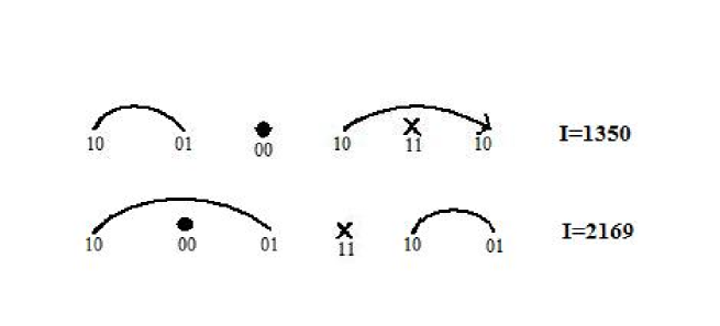
Figure 1: Representation of VB diagrams for a half-filled 6 orbital (site) system. Here $\bullet$ denotes empty site, $\times$ denotes doubly occupied site. The top VB diagram shows a spin pairings to yield a state with total spin $S_{tot}$=1, its bit representation corresponds to a unique integer I = 2350. The bottom VB diagram shows a $S_{tot}$ = 0 state, the corresponding unique integer, I is 2169.

We can generate the complete set of VB states for our case of $N$ orbitals with $N_{e}$ electrons of total spin $S$ and z-component of total spin $M_{S}=S$ by exhausting all possible occupancies of orbitals which satisfy $2S=N_{\uparrow}-N_{\downarrow}$. Since an orbital can be in any one of four states (empty, doubly occupied, a singlet line beginning or a singlet line ending, sites involved in an arrow being treated as line beginnings) we can use two bits to represent the state of an orbital. Thus, each VB diagram can be uniquely represented as an integer on a computer.

A line in the VB diagram, between sites $``i"$ and $``j"$, represents ${(\hat{a}^{\dagger}_{i,\alpha}\hat{a}^{\dagger}_{j,\beta}-\hat{a}^{\dagger}_{i,\beta}\hat{a}^{\dagger}_{j,\alpha})|0>}$/$\sqrt{2}$, where we choose $\alpha$ to correspond to $|\uparrow\rangle$ and $\beta$ to $|\downarrow\rangle$ orientations of the electron. The doubly occupied site $``i"$ corresponds to the state $a^{\dagger}_{i,\alpha}\hat{a}^{\dagger}_{i,\beta}|0>$. The phase convention assumed for a line between sites $``i"$ and $``j"$ is that the ordinal number $``i"$ is less than the ordinal number $``j"$. The $2S$ singly occupied sites $k_{1}$ $k_{2}$ $k_{3}$ . . . . $k_{2S}$ in the arrow represent the state with $M_{S}=S$ given by $\hat{a}^{\dagger}_{k_{1},\alpha}\hat{a}^{\dagger}_{k_{2},\alpha}\hat{a}^{\dagger}_{k_{3},\alpha}...\hat{a}^{\dagger}_{k_{2S},\alpha}|0>$. VB states corresponding to other M_S value for this state with spin S, can be obtained by operating, required number of times by the S${}_{tot}^{-}$ operator on the state. Since Hamiltonian in Eq.(1) is isotropic, each eigenstate in the spin S sector is (2S+1) fold degenerate and, by Wigner-Eckart theorem [17] it is sufficient to work in subspace of chosen M_S value. The VB state corresponding to a given diagram is a product of the states representing the constituent parts of the diagram, in no particular order as each part is either a product of two Fermion operators or a linear combination of the product of two Fermion operators.

Given the definition of a line in the VB diagram, every VB diagram, $|\psi_{i}>$ can be broken up into a linear combination of the constant $M_{S}$ basis states {$|\phi_{j}>$} as,

$$|\psi_{i}>=\sum_{j}C_{ij}|\phi_{j}>$$ (3)

A VB diagram with $n$ singlet lines yields $2^{n}$ basis states in the constant $M_{S}$ basis. To effect the conversion of VB diagrams to constant $M_{S}$ functions, we note that each singlet line gives two states; in one state, the site at which a singlet line begins is replaced by an $\alpha$ spin while the one at which it ends by a $\beta$ spin with phase +1 and in the other the spins are reversed and the associated phase is -1. There is a normalization constant, $(2^{-n/2}$, associated with the constant $M_{S}$ basis state. The matrix relating the VB basis states to constant $M_{S}$ basis states, C, is a $V\times M$ matrix, where $V$ is the dimensionality of the VB space and $M$ that of the constant $M_{S}$ space. If R_M the matrix representation of symmetry operation $\hat{R}$ is known, in constant $M_{S}$ basis, then the knowledge of the matrices C and R_M gives the result of operating by the symmetry operator $\hat{R}$ on a VB state as a linear combination of the constant $M_{S}$ basis states via the matrix B${}_{\hat{R}}$ = CR_M. The projection operator for projecting out the basis states on to a chosen irreducible representation $\Gamma$ of the point group is given by,

$$\hat{P}_{\Gamma}=\sum_{\hat{R}}\chi_{\Gamma}^{irr}({\hat{R}}){\hat{R}}$$ (4)

where, $\chi_{\Gamma}^{irr}(\hat{R})$ is the character under the symmetry operation $\hat{R}$ of the point group of the system [21]. The matrix representation of $\hat{P}_{\Gamma}$ in the mixed VB and constant $M_{S}$ basis is given by,

$${\mathbf{Q}_{\Gamma}}=\sum_{\hat{R}}\chi_{\Gamma}^{irr}(\hat{R}){\mathbf{B}_{\hat{R}}}$$ (5)

where, Q_Γ is a $V\times M$ matrix. However, the rows of the matrix Q_Γ are not linearly independent, since the complete symmetrized basis transforming as $\Gamma$ spans a much smaller dimensional Hilbert space. The exact dimension V_Γ of the Hilbert space spanned by the system in the irreducible representation $\Gamma$ can be known a priori and is given by,

$$V_{\Gamma}=(d_{\Gamma}/h)\sum_{\hat{R}}\chi^{red}(\hat{R})\chi_{\Gamma}^{irr}(\hat{R})$$ (6)

where $d_{\Gamma}$ is the dimensionality of the irreducible representation $\Gamma$, $h$ is the number of symmetry elements in the point group and $\chi^{red}(\hat{R})$ is the reducible character for the operation $\hat{R}$. The determination of $\chi^{red}(\hat{R})$ is nontrivial and the method of computing it will be discussed in the next subsection. The $V_{\Gamma}\times M$ projection matrix, P_Γ of rank $V_{\Gamma}$ is obtained by Gramm-Schmidt orthonormalization of the rows of the matrix Q_Γ until $V_{\Gamma}$ orthonormal rows are obtained. These orthonormal and linearly independent rows yield the desired linear combinations which transform as $\Gamma$ and also have total spin $S$. Projection matrix P_Γ is represented by these $V_{\Gamma}$ rows.

The $M\times M$ Hamiltonian matrix H_M is constructed in the constant $M_{S}$ basis (see subsection 2.1). Since the basis states in this representation are orthonormal, we do not encounter the problem of $``illegal"$ VB states. In the pure VB method, the Hamiltonian operating on a legal VB state can yield illegal VB diagrams which then need to be re-expressed as linear combination of the legal VB functions [19]. The $V_{\Gamma}\times V_{\Gamma}$ Hamiltonian matrix in the fully symmetrized basis is given by P_ΓH_M ${\bf P}_{\Gamma}^{\dagger}$ and one could use any of the well known full diagonalization routines to obtain the full eigenspectrum or use the Rettrup modification of Davidson algorithm [22] to get a few low-lying states of the symmetrized block Hamiltonian in the chosen spin and symmetry subspace.

For degenerate irreducible representations, such as the E, T, G or H representations, the above procedure does not lead to the smallest block of the Hamiltonian matrix. In such cases, it is advantageous to work with bases that transform according to one of the components of the irreducible representation. In case of E, T or H, this can be achieved by choosing an axis of quantization and projecting out basis states of the irreducible representation which are diagonal about a rotation about the quantization axes. For example, in the case of the irreducible representation that transforms as T, we can choose one of the C₃ axes as a quantization axis and project the basis states which transform as the irreducible representation T, using $(I+C_{3}^{1}+C_{3}^{2})$ as the projection operator. This operator projects states that transform as the Y${}_{1}^{0}$ component of the three fold degenerate irreducible tensor operator. Similarly we can choose a $C_{5}$ axis and use $(I+C_{5}^{1}+C_{5}^{2}+C_{5}^{3}+C_{5}^{4})$ as projection operator for the irreducible representation H. For the E representation, we can use $(I+C_{2})$ as projection operator with a chosen $C_{2}$ axis. The case of G is a bit tricky; one has to choose two $C_{2}$ axes, orthogonal to each other. The projection operator for this case then would be: $(I+C_{2})(I+C^{\prime}_{2})$. After these projection operations, dimensions of the Hamiltonians to be diagonalized would be half, one third, one fourth or one fifth respectively for the E, T, G and H representations.

Here we wish to emphasize the computational advantage of our technique over the constant $M_{S}$ basis method. The additional steps involved in the hybrid VB-Constant M_S method are (i) construction of the C matrix and (ii) computation of the B${}_{\hat{R}}$ matrix. However, if we wish to compute the properties of a state expressed as a linear combination of VB diagrams, the simplest way is to use the C matrix to transform the state from the VB basis to the constant $M_{S}$ basis. Therefore, construction of the C matrix is not strictly an overhead. Besides,the construction of the C matrix is a very fast step as the row index of the C matrix is the index of the VB state which we wish to decompose and the column indices of elements in this row are the indices of the resultant constant M_S states. The constant M_S states are easily generated as an ordered sequence of integers which represent them and this facilitates searching for the column index of the matrix. The coefficients will have a magnitude of $2^{-n/2}$ where $n$ is the number of lines in the $i^{th}$ VB diagram; the phase of the coefficient is easily fixed based on the phase convention used for a singlet line. In the hybrid approach, computation of the B${}_{\hat{R}}$ matrix involves the matrix multiplication, CR_M. The number of arithmetic operations involved is however very small, since both C and R_M are sparse matrices with the latter having only one nonzero matrix element per row. In both constant M_S and hybrid approaches one has to obtain the projection matrix P_Γ by retaining only the orthogonal rows of the matrix Q_Γ. Since the number of orthogonal rows in Q_Γ is far fewer than in R_M, this step is faster in the hybrid approach than in the constant $M_{S}$ approach by a factor D($\Gamma_{S}$)/D($\Gamma_{M_{S}}$), where D($\Gamma_{S}$) is the dimensionality of the space of the irreducible representation $\Gamma$ with spin S and D($\Gamma_{M_{S}}$) is similarly the dimension of the space $\Gamma$ with constant M_S. Though, this advantage is largely off-set by the fact that the R_M matrix in constant $M_{S}$ basis is more sparse than the Q_Γ matrix in the hybrid approach. Computation of the eigenvalues (diagonalization of Hamiltonian) in the constant $M_{S}$ approach is slower than in the hybrid approach, since D($\Gamma_{M_{S}}$)$>$D($\Gamma_{S}$) for most S (for example see Table 1). The memory required for the hybrid approach is not very different from that of constant $M_{S}$ approach, even though the matrices in the hybrid approach are slightly denser, they are smaller in size. The only additional memory demand in the hybrid approach is the storage of sparse C matrix. The major advantage of the hybrid approach is that we can obtain a far richer spectrum, since we are targeting each spin sector separately, unlike in the constant $M_{S}$ approach. Thus, if we can obtain (by our approach), say 10 states in each S sector, then each one will correspond to a unique state. There will be no repetition of the states. But in contrast, 10 states obtained in a $M_{S}$ sector (by constant $M_{S}$ approach) may not be unique, since many of these states would be repeated in different $M_{S}$ sectors.

2.1 Implementation Details

We can represent a basis uniquely by a 2N-digit binary number [11] (N is the number of sites / orbitals); the first two bits describe the state of the first site, next two bits describe the state of the second and so on. For constant $M_{S}$ basis, we use the bit states “00” for an empty site, “10” for site with spin-up electron, “01” for site with spin-down electron and “11” for a doubly occupied site. Similarly, for VB basis, we use “00” for empty site, “10” for a singlet line-beginning at a site as well as for all sites in the arrow, “01” for a line-ending and “11” for a doubly occupied site. The Rumer-Pauling rules are implemented by enforcing that for a given site $``i"$, the quantity (# of line beginnings - # of line endings) at sites one to $i-1$ should be $\geq 0$ [18]. Our binary coding implies that the number of bits in the state “1” is equal to the number of electrons $N_{e}$. To generate integers that represent VB states, we generate integers with $N_{e}$ “1” bits in the bit field from zero to (2N-1) in increasing sequence and check to see if the bit pattern corresponds to a “legal” VB diagram with chosen total spin. For integers corresponding to constant $M_{S}$ basis, total $M_{S}$ value should be the desired value and the Rumer-Pauling condition is not enforced. The positive integers so generated uniquely represent the states of the VB or constant $M_{S}$ bases.

Computationally, finding the transformation matrix C which carries the VB basis to constant $M_{S}$ basis is straightforward. We initialize the coefficients in the row of the matrix C corresponding to the chosen VB state to zero. We then decompose the VB diagram by converting every singlet line in the diagram into two $M_{S}$ states. The indices of the resulting constant $M_{S}$ states correspond to the column indices of C and are determined by a binary search on the list of integers that represent the constant $M_{S}$ states. The corresponding matrix element is given by the normalized VB coefficient with appropriate phase. On a computer, the transformation matrix C is stored in sparse form. Next, we construct the projection matrix (P_Γ), by constructing the matrix representation of each of the symmetry operators, $\hat{R}$, of the point group in the constant $M_{S}$ basis. This is achieved by (i) obtaining the occupancies of each site from the integer representing the basis state, and (ii) by letting $\hat{R}$ act on the basis state by appropriately rearranging the sites together with their occupancies to obtain the new bit pattern corresponding to the resultant state. The new occupancy pattern is converted into the integer representing the state and fixing the column index of the matrix R by a binary search for the index of the new integer in the list of integers representing the constant $M_{S}$ basis. Care should be taken to keep track of the phase factor while interchanging the occupancies since Fermion creation operators anticommute. From a knowledge of C and all the R_M matrices we can construct the matrix ${\mathbf{Q}_{\Gamma}}$ (Eq. 5). But the rows of ${\mathbf{Q}_{\Gamma}}$ are in general not linearly independent, eliminating linear dependencies leads to the projection matrix P_Γ with V_Γ number of linearly independent rows. The V_Γ linearly independent rows can be obtained by (i) collecting all linearly independent rows, by inspection, by noting that the set of rows which are disjoint (that is do not have non zero elements with common column index) are orthogonal by virtue of the fact that the constant $M_{S}$ basis sets are orthogonal and (ii) by carrying out Gram-Schmidt orthonormalization to obtain the remaining linearly independent rows. However, knowing V_Γ a priori is important to be able to stop the orthonormalization process once the number of linearly independent rows obtained equals the dimensionality of the symmetrized space. While V_Γ can be obtained from Eq. 6, it needs a knowledge of the reducible character.

To obtain the reducible character, it appears that we need a matrix representation of the symmetry operator in the VB basis. Given an operator $\hat{R}$, the matrix representation r, in the VB basis, is obtained from,

$$\hat{R}|\psi_{i}>=\sum_{j}r_{ij}|\psi_{j}>.$$ (7)

However, since the VB basis is non-orthogonal, we need the inverse of the overlap matrix,S^-1, where S${}_{ij}=<\psi_{i}|\psi_{j}>$ are the matrix elements of S. The matrix r is then given by RS^-1, where the matrix elements of R are given by $R_{ij}=<\psi_{j}|\hat{R}|\psi_{i}>$. In general determination of the matrix S^-1 is difficult for Fermionic systems and computationally prohibitive for large pure spin systems.

The above difficulty can be circumvented by resorting to the bit representation of VB and constant $M_{S}$ basis states. Using the C matrix, we can rewrite 7 as

$$\hat{R}|\psi_{i}>=\sum_{j}r_{ij}\sum_{k}C_{jk}|\phi_{k}>.$$ (8)

For every state $|\psi_{i}>$, we need to find the coefficient $r_{ii}$ and the reducible character $\chi^{red}(\hat{R})=\sum_{i}r_{ii}$. Taking the inner product on both sides of Eq. 8 with $|\phi_{l}>$,we get,

$$<\phi_{l}|\hat{R}|\psi_{i}>=\sum_{j}\sum_{k}r_{ij}C_{jk}<\phi_{l}|\phi_{k}>~{}~{}~{}~{}~{}~{}~{}$$ (9)

$$=\sum_{j}r_{ij}C_{jl}~{}~{}~{}~{}~{}~{}~{}~{}~{}~{}~{}~{}~{}~{}~{}~{}~{}~{}~{}~{}~{}~{}~{}~{}~{}~{}~{}~{}~{}$$

$r_{ij}$ are unknowns and need to be determined. The $lhs$ can also be evaluated as

$$<\phi_{l}|\hat{R}|\psi_{i}>=<\phi_{l}|\hat{R}|\sum_{j}C_{ij}|\phi_{j}>~{}~{}~{}~{}~{}~{}~{}~{}$$ (10)

$$=\sum_{j}C_{ij}\sum_{k}R_{jk}<\phi_{l}|\phi_{j}>$$

$$=\sum_{k}R_{lk}C_{il}~{}~{}~{}~{}~{}~{}~{}~{}~{}~{}~{}~{}~{}~{}~{}~{}~{}~{}~{}~{}~{}~{}~{}$$

where $R_{ij}$ is the matrix representation of $\hat{R}$ in the constant $M_{S}$ basis which is known. The only unknowns on the $rhs$ of Eq. 9 are the coefficients $r_{ij}$ and we need to determine the diagonal elements $r_{ii}$.

To determine $r_{ii}$, let us first assume that integers $\{J_{l}\}$ represent the constant $M_{S}$ basis states $\{|\phi_{l}>\}$ and the integers $\{I_{i}\}$ represent the VB states $\{|\psi_{i}>\}$. Now we note that in the expansion of a VB state $|\psi_{i}>$ as a linear combination of constant $M_{S}$ states (Eq. 3), the largest integer that represents the constant $M_{S}$ state, $J_{l}$ which appears in the expansion, is the one corresponding to the integer that represents the VB state $|\psi_{i}>$ itself, namely $I_{i}$. This is because, we have chosen the bit state “10” both for a line beginning in the VB state and for an up spin occupancy in the constant $M_{S}$ basis. The assertion that $I_{i}\geq J_{j}$ in the decomposition of the VB state $|\psi_{i}>$ into constant $M_{S}$ functions $|\phi_{j}>$, implies that the matrix C has nonzero elements $C_{jk}$ only for $J_{k}\leq I_{j}$.

Let us consider Eq. 7, we note that on the rhs the summation runs over all the states of the VB basis. Let us consider the VB state, $|\psi_{V}>$ which is represented by the largest permitted integer, $I_{V}$. This integer also correspond to the $M_{S}$ basis state $|\phi_{M}>$ (where $M$ is the dimensionality of the constant $M_{S}$ space) with the largest integer representation, ($I_{V}=J_{M})$, Taking the inner product with the state $|\phi_{M}>$, from Eq. 10 and Eq. 9, we obtain,

$$<\phi_{M}|\hat{R}|\psi_{i}>=r_{i,V}C_{V,M}$$ (11)

All other terms on the rhs of Eq. 9 are zero. Hence using Eq. 11, we can determine $r_{i,V}$. We can now proceed with the constant $M_{S}$ state whose representing integer $J_{K}$ is equal to $I_{V-1}$. The constant $M_{S}$ state with $J_{K}$ can appear only in the expansions of the VB states $\psi_{V}$ and $\psi_{V-1}$. Taking the inner product with $\phi_{K}$, we obtain,

$$<\phi_{K}|\hat{R}|\psi_{i}>=r_{i,V}C_{V,K}+r_{i,V-1}C_{V-1,K}$$ (12)

In 12, the only unknown is $r_{i,V-1}$ and can be evaluated. Similarly, by proceeding to the VB state $\psi_{V-2}$, we can obtain $r_{i,V-2}$. We can terminate when we reach the VB state $|\psi_{i}>$. This procedure can be adopted to obtain all the diagonal elements of the r matrix and hence the reducible character, $\chi^{red}$.

Constructing the Hamiltonian matrix in constant $M_{S}$ basis in real space is a fast and easy step. The basis states are eigenstates of the interaction part for the model Hamiltonians. From the binary sequence of the integers which represent the constant $M_{S}$ basis, we know the occupancy of each site and hence the diagonal contribution of the interaction terms. Simple rules for operating on a constant $M_{S}$ basis state by the operators $\hat{E}_{ij}=\sum_{\sigma}(\hat{a}^{\dagger}_{i\sigma}\hat{a}_{j\sigma}+\hat{a}^{\dagger}_{j\sigma}\hat{a}_{i\sigma})$ have been published elsewhere and together with a binary search procedure which allows rapid generation of the matrix corresponding to the one-electron terms of the Hamiltonian [11].

3 Application to Icosahedral Cluster

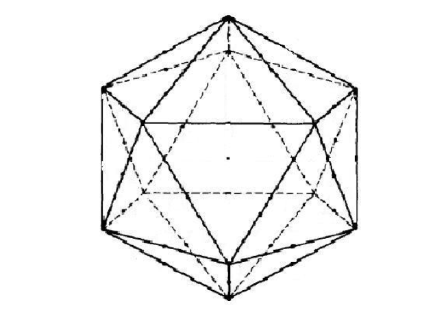
Figure 2: Regular icosahedron with ($I_{h}$) symmetry. Our system has an orbital at each of the 12 vertexes, and a transfer integral corresponding to a bond on each of the 30 edges; In the PPP model, the bond length is taken to be 1.4 Å.

To illustrate the power of our technique, we have applied the method to a 12-site regular icosahedral cluster (see Fig. 2) at half-filling. It has 30 edges (each one here taken to be of length 1.4 Å) representing a chemical bond.We have chosen this system, because it belongs to very high symmetry non-Abelian point group and presents a very general case for testing our method. This point group is also the same as the point group of the $C_{60}$ molecule. So properties, which are particularly symmetry-related, obtained for our model system, would also be useful in gaining insights into the $C_{60}$ molecule.

We have studied the icosahedron within the Hubbard model in which the inter-site interactions are neglected, for a range of $U$ values, as well as in the PPP model with standard Carbon parameters. The number of $M_{S}$=0 states is 853,776 and we have obtained the exact energies of all the states, by using the full spatial and spin symmetries of the system. The energies of $M_{S}\neq 0$ states are also known, since we know the total spin of each state. We have studied the density of states in each symmetry and spin sector as a function of $U$ in the Hubbard models and also for standard parameters in the PPP model.

In Table (1), we give the dimensions of all the subspaces of different total spin and total $M_{S}$ values, for the Icosahedral cluster.

Table 1: Dimensionalities of different spin subspaces of a half-filled 12-site (orbital) electronic system. $D(S)$ is the dimensionality of the constant S basis and $D(M_{S})$ is the dimensionality of the constant $M_{S}$ basis.

S/MS	0	1	2	3	4	5	6
$D(S)$	226512	382239	196625	44044	4212	143	1
$D(M_{S})$	853776	627264	245025	48400	4356	144	1

We note here the huge fall in size of total spin subspaces compared to total $M_{S}$ subspaces for most of the cases. Using the hybrid VB-constant $M_{S}$ method, we have broken down each total spin sectors into basis states that transform as different irreducible representations of the icosahedral point group. The dimensionalities of the various symmetry subspaces are shown in Table (2).

Table 2: Dimensionalities of different symmetry and spin subspaces of half-filled icosahedral cluster.

S${}_{tot}\rightarrow$
$\Gamma$ $\downarrow$	0	1	2	3	4	5	6
Ag	2040	3128	1684	382	38	3	1
T1g	16602	28821	14625	3261	309	6	0
T2g	16602	28821	14625	3261	309	6	0
Gg	30272	50932	26236	5880	568	16	0
Hg	47940	79305	41255	9220	900	40	0
Au	1852	3188	1644	348	40	0	0
T1u	17082	28686	14700	3372	294	18	0
T2u	17082	28686	14700	3372	294	18	0
Gu	30160	50992	26176	5888	560	16	0
Hu	46880	79680	40980	9060	900	20	0
Tot Dim $\rightarrow$	226512	382239	196625	44044	4212	143	1

We note that most subspaces are small enough for obtaining all the eigenstates of the Hamiltonian. However, for degenerate representations the subspaces are large and can be reduced by a factor equal to the dimensionality of the representation, as described earlier. We have used this approach and obtained all the eigenstates of the ensuing Hamiltonian matrix using a full matrix diagonalization routine. Since the number of eigenstates in each subspace is large, we have computed the density of states (DoS) using a $\Delta$E of 0.4eV, for which the histograms of the DoS are stable. A histogram for particular spin is evaluated by summing over corresponding states of all symmetries. Same is for histogram for particular symmetry, where corresponding states of all spins are considered. Although, unlike the one-particle DoS, the many-body DoS is not an intensive quantity. However, for a given model and system size, we can use these quantities to understand the behavior of the system.

3.1 Hubbard model studies

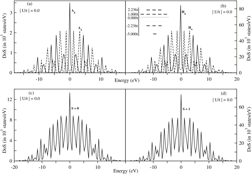
Figure 3: DoS profiles for (a) A_g and A_u and (b) H_g and H_u spaces. For other symmetry subspaces, the DoS profiles are similar. We note the difference in profiles for $g$ and $u$ spaces. DoS profiles for (c) S = 0 and (d) S = 1 are also given. Inset of (b) gives the one-particle spectrum for the regular icosahedron in the Hückel model.

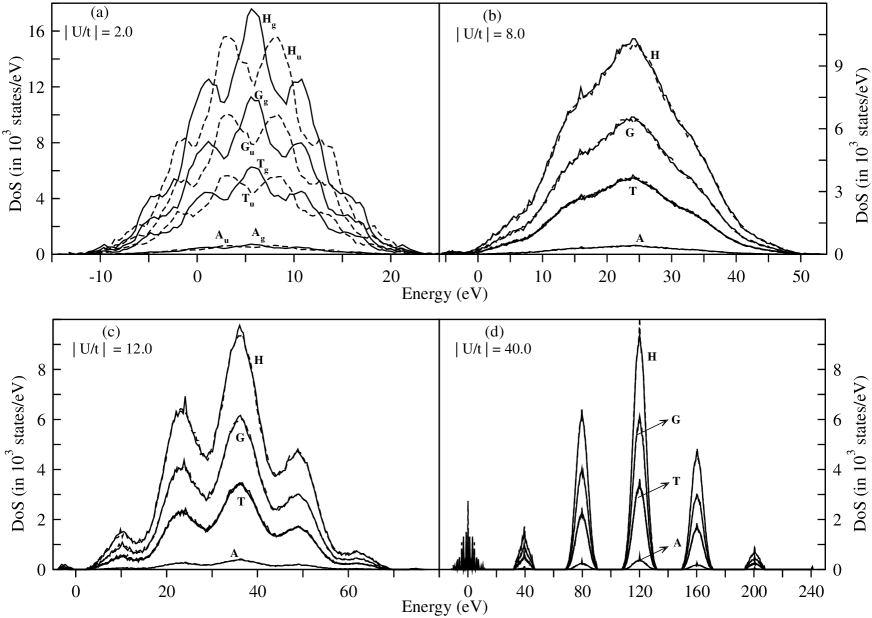
Figure 4: DoS profiles in various symmetry subspaces for four different $|U/t|$ values are shown. Note, in (a), profiles for T_1g and T_2g coincide and simply referred to as T_g. Same is for the triply degenerate $u$ space. In (b), (c) and (d), DoS profiles for corresponding $u$ and $g$ spaces coincide, so they are referred to by their common irreducible representation symbols.

In Fig. (3), we show the many-body DoS for the Hückel model in the the various $A_{g},~{}H_{g}$ and $A_{u},~{}H_{u}$ spaces. Here, we have summed over all spin states, for simplicity. We have also shown the DoS plots of different spin space, in which they are summed over all the irreducible spaces. Two things are worth noting. Firstly, the DoS displays a symmetry about zero of energy in each of the subspaces, even though the system does not possess the e-h symmetry. In fact, it is clear from the one particle spectrum that there is no symmetry in the one-particle energy levels about zero energy. Secondly, the DoS profile of the $g$ subspace shows peaks where ever there is a valley in the DoS profile of the $u$ subspace. This is indeed true also for other irreducible representations not shown in the figure. The reason for this symmetry in the DoS plots is because the sum of the one particle eigenvalues are zero and follows from the fact that in Hückel model, with all site energies set to zero, the diagonal matrix elements are all zero. This implies $\sum_{i}2\epsilon_{i}~{}=~{}0$, where $\epsilon_{i}$ are the molecular orbitals (MO) energies. Thus, for any given occupancy pattern of the MOs at half-filling, we have $\sum_{i}n_{i}\epsilon_{i}~{}=~{}-\sum_{i}(2-n_{i})\epsilon_{i}$ and since $\sum_{i}n_{i}=\sum_{i}(2-n_{i})$, at half filling, we find that for every many-body state of energy $E_{k}$ there exists a many-body state of energy $-E_{k}$, even though the MO energies $\epsilon_{i}$ do not satisfy the pairing theorem [20]. Thus, the symmetry in DoS plots is not a consequence of the pairing theorem but due to the fact that the magnitude of the sum of the energies of the bonding MOs is equal to the magnitude of the sum of the energies of anti-bonding MOs. This is in fact a general result for the Hückel model with equivalent sites. The second observation about the location of valleys and peaks in the DoS of the states with $g$ and $u$ symmetries is due to the fact that the molecular orbital occupancies which give the $g$ and $u$ representations are different due to symmetry considerations. The DoS plots in various spin subspaces are also shown in Fig. (3). We find that they show several peaks in each total spin space. We show in Fig. (4) DoS profiles for the Hubbard model in various symmetry subspaces for different values of $|U/t|$ and in Fig. (5) we show the same in different total spin spaces. The evolution of DoS with correlation strength is interesting. Firstly, we note that for $|U/t|=2.0$, the sharp peaks in the DoS found in the Hückel model are broadened. The peaks in the $g$ subspace coincide with the troughs in the $u$ symmetry and vice versa. The ground state energy in the presence of correlations is higher than in the Hückel model, as expected.

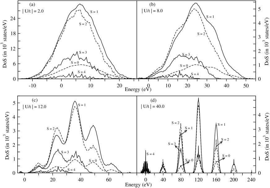
Figure 5: DoS profiles of various spin subspaces for four different $|U/t|$ values are shown.

In the very strong correlation regime, ($|U/t|=12$ and $|U/t|=40$ we again find peaks in the DoS in all the subspaces. What is interesting is that peaks appear at almost the same value of energy in $g$ and $u$ subspaces, unlike in the non-interacting or weakly interacting model, and are approximately $|U/t|$ apart in energy. This can be understood by noting that the many body space can be subdivided into space of all singly occupied sites; space of one empty, one doubly occupied and rest singly occupied sites; space of two empty, two doubly occupied and rest singly occupied sites and so on. The interaction energies of these class of states is 0, $U$, $2U$, etc. The transfer term leads to weak admixture of these states, and in the strong correlation limit results in broadening of the DoS peaks centered at the energies 0, $U$, $2U$ etc. Thus, the DoS plots, although look similar in both the small $|U/t|$ and the large $|U/t|$ limits, their origin as well as their location is different. It is also worth noting that the DoS curves centered at different energies are similar for all the subspaces. However, in the large $|U/t|$ limit, the DoS curves for the same total spin centered around different energies are not similar, showing that we do not have a strict spin-charge separation in icosahedron in this limit. For, if indeed we had such a separation, we would expect very similar DoS for the same total spin, for different number of doubly occupied sites, when the allowed number of total spin states is large.

For $|U/t|=8.0$, the DoS is very different. We find that there is a single broad peak and all the other peaks are small inflexions superimposed over the peak. The ”band width” of the one-particle spectrum (see Fig. 3b, inset) is $7.236t$ and the Hubbard correlation strength is very close to this value. Thus, for an icosahedral cluster, the parameters are at the intermediate correlation regime and leads to a smearing of the structure which is found at the weak and strong correlation limits. However, independent of the correlation strength, we find that the DoS curves are nearly identical for the T_1g and T_2g spaces and also for the T_1u and T_2u spaces.

Table 3: Lowest and second lowest energies for each symmetrized spin sector (for PPP model). All energies are in eV.

S${}_{tot}\rightarrow$	0	1	2	3	4	5	6
$\Gamma$ $\downarrow$
Ag	0.000	8.154	5.600	9.976	16.871	40.390	36.724
	1.533	8.835	8.618	15.601	26.400	42.449	$-$
T1g	0.912	0.672	5.918	9.011	18.255	40.390	$-$
	6.660	1.249	8.726	10.594	18.620	42.449	$-$
T2g	0.830	0.665	5.878	9.042	18.577	40.390	$-$
	6.228	1.229	9.007	10.171	19.058	42.449	$-$
Gg	0.058	0.134	5.485	8.631	17.626	30.589	$-$
	1.178	0.638	6.891	9.015	18.281	41.322	$-$
Hg	0.777	0.122	0.279	8.895	16.967	26.206	$-$
	0.831	1.393	5.401	9.160	17.609	30.428	$-$
Au	2.339	3.502	2.713	12.029	21.755	$-$	$-$
	3.725	4.274	7.900	16.492	26.126	$-$	$-$
T1u	3.846	2.349	2.937	6.888	20.761	31.775	$-$
	4.051	2.844	6.943	11.175	24.184	35.225	$-$
T2u	2.653	2.382	2.854	10.950	21.087	23.484	$-$
	4.111	2.773	7.506	11.929	24.249	32.728	$-$
Gu	2.724	2.233	2.630	10.982	15.232	33.555	$-$
	3.461	2.690	4.005	11.857	20.867	38.355	$-$
Hu	2.225	2.372	2.414	11.638	15.747	33.469	$-$
	2.795	2.676	2.689	11.881	20.653	38.586	$-$

3.2 PPP model studies

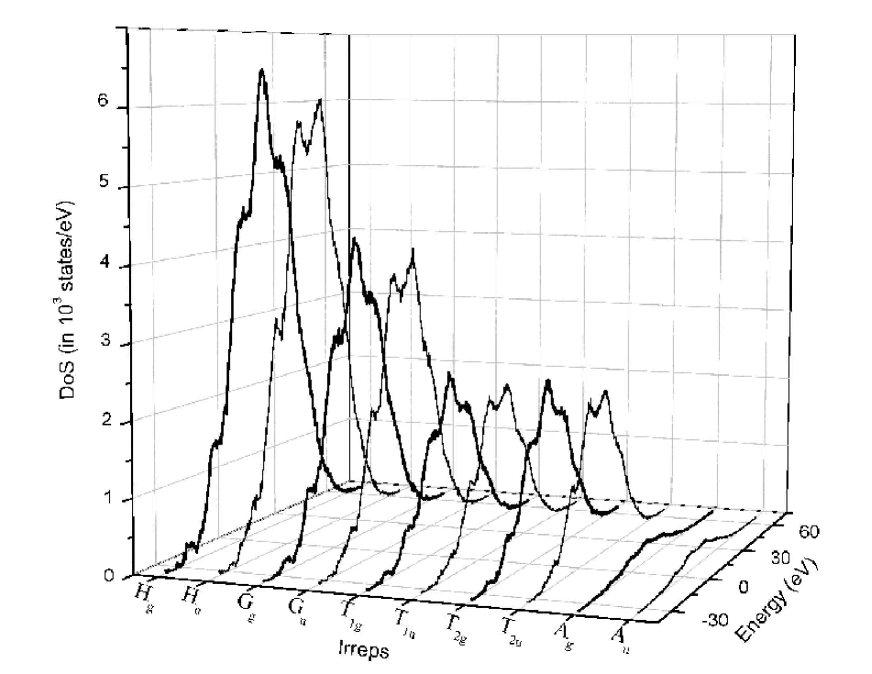
Figure 6: DoS profiles of various symmetry subspaces for PPP model.

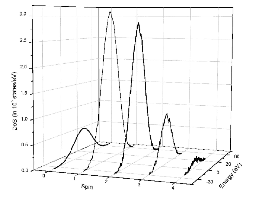
Figure 7: DoS profiles of various spin subspaces for PPP model.

The Hubbard model is not the appropriate model for studying carbon systems as it neglects long-range interactions. The appropriate model for studying such systems is the PPP model, which we have employed for studying the cluster.

In Table (3), we show two lowest energy levels in each of the subspaces. We note that the ground state is the lowest energy state in the $A_{g}$ subspace with total spin zero. The one-photon gap is given by the lowest energy excitation to the $T_{1u}$ space for an Icosahedron. Thus, we find that lowest excitation gap is at energy of 3.846 eV. This can be compared with the excitation gap of 3.552 eV for a PPP chain of 12 carbon atoms [23]. We do not compare the excitation gaps to PPP ring of 12 carbon atoms, as the $N=4n$ ($n$ integer) have very strong finite size effects due to degenerate partly filled highest occupied molecular orbitals. The second allowed excitation is at an energy of 4.051 eV. The two photon gap is to the second lowest energy state in the $A_{g}$ representation and is found to be 1.533 eV which is very low compared to a polyene chain ($\sim$ 3.0 eV).

The lowest energy spin gap, from the singlet ground state is to the lowest energy spin 1 state in the $H_{g}$ space. This gap is 0.122 eV which is very low compared to the polyenes. In general, the singlet-triplet gaps in conjugated systems is about 60% the optical gap and icosahedron seems to be an exception. Since singlet-triplet gap here is much higher compared to room temperature enery (about 0.025 eV), the system would show diamagnetic behavior below this temperature. There is also another triplet state which is about 0.012 eV above the lowest energy triplet state. These observations imply that the icosahedral cluster would exhibit paramagnetism above room temperature due to significant population of these states. Based on the similar argument, we also conclude that the specific heat at low-temperature will be very small and increase exponentially with increasing temperature. The triplet-triplet (TT) excitation from the $H_{g}$ space is to states in $T_{1u},~{}T_{2u},~{}G_{u}~{}\rm{and}~{}H_{u}$ while from the $G_{g}$ state is to states $T_{2u}$, $G_{u}$ and $H_{u}$. This means that we would have a band of TT excitations starting from 2.11 eV. Regarding higher spin excitations, there is a low energy quintet state about 0.279 eV above the ground state and a few other quintet excitations of energies between 2.414 and 2.937 eV. All other spin excitations are very high energy excitations, as the higher spin states have very low kinetic stabilization.

In Figs. (6) and (7), we show the density of states plots for different symmetry subspaces and different total spins. We note from the figures that the icosahedral cluster of conjugated Carbon atoms belongs to the weakly correlated regime since the DoS peaks in the $g$ and $u$ spaces do not coincide in energy. We also find that this conclusion is corroborated by the DoS plots for different total spin states. The $S=0$ DoS plot shows a featureless broad peak, as seen for small $|U/t|$ values of the Hubbard model. The higher spin states also show broad peaks consistent with the weak correlation regime. Even in the PPP model, the DoS plots for the $T_{1g}$ and $T_{2g}$ are very similar and same is the case with the $T_{1u}$ and $T_{2u}$ states. These DoS plots would also indicate the nature of the electronic spectra in these systems.

One of the most fascinating molecules to have been discovered is C₆₀, which also has icosahedral symmetry. The Hückel band width of C₆₀ is 5.618 $t$, when the transfer integrals for the hexagon-pentagon and the hexagon-hexagon bonds are taken to be the same. This is much smaller than the 7.236 $t$ found for icosahedron. This is largely due to the different number of bonds per site (2.5 bonds / site for icosahedron compared to 1.5 bonds / site for C₆₀) in the two systems. For this reason, we expect PPP model with standard parameters of C₆₀ to be in a more strongly correlated regime than the icosahedron. This should also reflect in the electronic spectra of C₆₀. The full spectrum of icosahedron will also be helpful in gaining insights into the contributions of different states to the linear and nonlinear optical response of the system.

4 Summary

In this paper, we have considered the long standing problem of both spacial and spin symmetry adaptation for arbitrary point groups. We have shown that by using the strengths of the VB and the constant $M_{S}$ methods, we can have a hybrid scheme which exploits the full symmetry of a non-relativistic Hamiltonian. We have illustrated this by applying to the nontrivial case of an icosahedral cluster. We have obtained all the eigenstates of the cluster by our method. The hybrid method is less demanding on both memory and CPU time of a computer and is easy to implement. We have obtained the DoS of the Hubbard model for different Hubbard parameters $U$ and of the PPP model for an icosahedral cluster. These plots show different characteristics as a function of interaction strength in the Hubbard model. The PPP model studies indicate that while the one-photon gaps are comparable with other conjugated systems, the spin gaps are unusually small. This may lead to significant population of the magnetic states at room temperature. These studies have a bearing on the C₆₀ system which also possesses icosahedral symmetry. The method discussed here will be of considerable importance in studying the dynamics and finite temperature properties of systems whose Hamiltonians are amenable to exact diagonalization. While we have illustrated the method using a highly symmetric Hamiltonian, the method is very general and applicable to systems belonging to any point group. In point groups with lower symmetry, while the advantage of automatically labeling the states exists, the actual savings in computational effort would be decreased.

5 Acknowledgments

This work was supported by Department of Science and Technology, Government of India, through various projects. We are also pleased to acknowledge Prof. Diptiman Sen for valuable discussions.

References

- [1] Sahoo, S.; Rajamani, R.; Ramasesha, S.; Sen, D. Phys Rev B 2008, 78, 054408.
- [2] Jensen, F. Introduction to Computational Chemistry; JOHN WILEY & SONS: UK, 1999; Chapter 4.
- [3] Salem, L. The Molecular Orbital Theory of Conjugated Systems; W. A. Benjamin, Inc.: New York, 1966.
- [4] Pariser, R.; Parr, R. G. J Chem Phys 1953, 21, 767.
- [5] Pople, J A Trans Faraday Soc 1953, 49, 1375.
- [6] Hubbard, J Proc Roy Soc A 1963, 276, 238.
- [7] Springborg, M. Methods of Electronic-Structure Calculations: From Molecules to Solids; JOHN WILEY & SONS: UK, 2000; Chapter 11.
- [8] Zerner, M. C. In Reviews In Computational Chemistry: Vol. 2; Lipkowitz, K. B.; Boyd, D. B., Ed.; WILEY-VCH: New York, 1991.
- [9] Ohno, K. Theor Chim Acta 1964, 2, 219.
- [10] Pauncz, R. Spin Eigenfunctions: Construction and Use; Plenum Press: New York, 1979.
- [11] Soos, Z. G.; Ramasesha, S. In Valence Bond Theory and Chemical Structure; Klein, D. J.; Trinajstic, N., Ed.; Elsevier: New York, 1990. Ramasesha, S.; Soos, Z. G. In Valence Bond Theory; Cooper, D. L., Ed.; Elsevier: 2002; chapter 20.
- [12] Lwdin, P.-O. Phys Rev 1955, 97, 1509.
- [13] Bernu, B.; Lecheminant, P.; Lhuillier, C.; Pierre, L. Phys Rev B 1994, 50, 10048.
- [14] Saxe, P.; Fox, D. J.; Schaefer, H. F.; Handy, N. C. J Chem Phys 1982, 77, 5584. Siegbahn, P. E. M. J Chem Phys 1980, 72, 1647. Brooks, B. R.; Schaefer, H. F. J Chem Phys 1979, 70, 5092. Robb, M. A.; Niazi, U. Comput Phys Rep 1984, 1, 127.
- [15] Duch, W.; Karwowski, J. Int J Quantum Chem 1982, 22, 783. Duch, W.; Karwowski, J. Comput Phys Rep 1985, 2, 93.
- [16] Pauling, L. J Chem Phys 1933, 1, 280. Pauling, L.; Wheland, G. W. ibid 1933, 1, 362.
- [17] Sakurai, J. J. Modern Quantum Mechanics; Addison-Wesley: USA, 1994; chapter 3.
- [18] Ramasesha, S.; Soos, Z. G. Int J Quantum Chem 1984, 25, 1003.
- [19] Ramasesha, S.; Soos, Z. G. J Chem Phys 1993, 98, 4015.
- [20] Coulson, C. A.; Rushbrooke, G. S. Proc Cambridge Phil Soc 1940, 36, 193.
- [21] Bishop, D. M. Group Theory and Chemistry; Clarendon Press: Oxford, 1973.
- [22] Davidson, E. R. J Comput Phys 1975, 17, 87. Rettrup, S. J Comput Phys 1982, 45, 100.
- [23] Soos, Z. G.; Ramasesha, S. Phys. Rev. B 1984, 29, 5410.