Reionization and feedback in overdense regions at high redshift

Abstract

Observations of galaxy luminosity function at high redshifts typically focus on fields of view of limited sizes preferentially containing bright sources. These regions possibly are overdense and hence biased with respect to the globally averaged regions. Using a semi-analytic model based on Choudhury & Ferrara (2006) which is calibrated to match a wide range of observations, we study the reionization and thermal history of the universe in overdense regions. The main results of our calculation are: (i) Reionization and thermal histories in the biased regions are markedly different from the average ones because of enhanced number of sources and higher radiative feedback. (ii) The galaxy luminosity function for biased regions is markedly different from those corresponding to average ones. In particular, the effect of radiative feedback arising from cosmic reionization is visible at much brighter luminosities. (iii) Because of the enhanced radiative feedback within overdense locations, the luminosity function in such regions is more sensitive to reionization history than in average regions. The effect of feedback is visible for absolute AB magnitude $M_{AB}\gtrsim-17$ at $z=8$, almost within the reach of present day observations and surely to be probed by the James Webb Space Telescope (JWST). This could possibly serve as an additional probe of radiative feedback and hence reionization at high redshifts.

1 Introduction

Deep surveys have now discovered galaxies at redshifts close to the end of reionization (Bouwens & Illingworth, 2006; Iye et al., 2006; Bouwens et al., 2007; Henry et al., 2007; Stark et al., 2007; Bouwens et al., 2008; Bradley et al., 2008; Henry et al., 2008; Ota et al., 2008; Richard et al., 2008; Bunker et al., 2009; Bouwens et al., 2009; Henry et al., 2009; McLure et al., 2009; Oesch et al., 2009; Ouchi et al., 2009; Bouwens et al., 2009; Ouchi et al., 2009; Sobral et al., 2009; Zheng et al., 2009; Oesch et al., 2010; Castellano et al., 2010; Bouwens et al., 2010; Hickey et al., 2010; McLure et al., 2010). Luminosity function of these galaxies, and its evolution, can answer important questions about reionization. Indeed, much work has been done on constructing self-consistent models of structure formation and the evolution of ionization and thermal state of the IGM that explain these observations (Choudhury & Ferrara, 2005; Haiman & Cen, 2005; Wyithe & Loeb, 2005; Choudhury & Ferrara, 2006; Dijkstra et al., 2007; Samui et al., 2007; Iliev et al., 2008; Samui et al., 2009). Studies of the Gunn-Peterson trough (Gunn & Peterson, 1965) at $z\geq 6$ have established that the mean neutral hydrogen fraction is higher than $10^{-4}$ (e. g. Fan et al. 2006) and it is most likely that the IGM is still highly ionized at these redshifts (Gallerani et al., 2008a, b). Furthermore, CMB observations indicate the electron scattering optical depth to the last scattering surface to be $\tau_{e}=0.088\pm 0.015$ based on the WMAP seven year data. A combination of high redshift luminosity function data with the data from these absorption systems and CMB observations favour an extended epoch of reionization that begins at $z\approx 20$ and ends at $z\approx 6$ (Choudhury & Ferrara, 2006).

Nonetheless, interpreting high redshift luminosity functions is not straightforward and detailed modelling is required. For instance, local HII regions around these galaxies can affect luminosity function evolution (Cen et al., 2005) and clustering of galaxies can enhance this effect (Cen, 2005). Another complication is because of the fact that these surveys can detect only the brightest galaxies at these high redshifts ($z\gtrsim 6$). Such galaxies can form only in highly overdense regions and therefore the surveyed volume is far from average. An important question in that case is whether reionization proceeds differently in such regions (Wyithe & Loeb, 2007).

Galaxy formation is enhanced in overdense regions because of a positive bias in abundance of dark matter haloes. The enhancement in the number of galaxies is proportional to the mass overdensity in the region, with the constant of proportionality (‘bias’) related to halo masses and collapse redshifts (Cooray & Sheth, 2002). This increases the number density of sources of ionising radiation and aids reionization of the intergalactic medium (IGM) in overdense regions. However, an increase in the IGM density also adds to radiative recombination. Furthermore, reionization is accompanied by radiative feedback (Thoul & Weinberg, 1996). Radiative feedback heats the IGM and suppresses formation of low mass galaxies. This increase in radiative recombinations and feedback works against the process of reionization and the two effects need not cancel out. Relative significance of these negative and positive contributions will determine how differently reionization evolves in overdense regions.

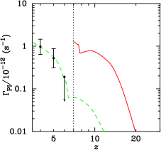
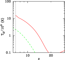
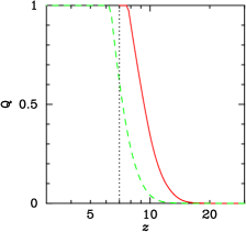
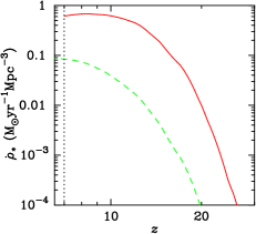
Figure 1: Behaviour of various quantities in our fiducial model, in the average and overdense regions are shown by dashed and solid lines respectively. The top left panel shows the photoionisation rate, with data points taken from (Bolton & Haehnelt, 2007). The top right panel shows the mass-averaged temperature for ionised regions, which essentially determine the radiative feedback. The bottom left panel is for the volume filling factor of ionised regions. The bottom right panel shows the cosmic star formation rate. Note that the overdense region that we consider here collapses at $z=6.8$. The vertical dotted line in the top left panel highlights this. We cannot evolve our reionization model for smaller redshifts.

Recently, Kim et al. (2009) studied a sample of $i_{775}$-dropout candidates identified in five Hubble Advanced Camera for Surveys (ACS) fields centred on Sloan Digital Sky Survey (SDSS) QSOs at redshifts $z\approx 6$. They compared results with those from equally deep Great Observatory Origins Deep Survey (GOODS) observations of the same fields in order to find an enhancement or suppression in source counts in ACS fields. An enhancement would imply that bias wins over negative feedback in these overdense regions. They found the ACS populations to be overdense in two fields, underdense in two field, and equally dense as the GOODS populations in one field. Somewhat surprisingly, they did not find a clear correlation between density of $i_{775}$ dropouts and the region’s overdensity.

In this paper, we use semi-analytic models to study reionization within overdense regions. The main aim of this work is to quantify the effects of enhancement in the number of sources and radiative feedback within such regions and explore the possibility whether the galaxy luminosity function in overdense regions can be used as potential probe of feedback and reionization history. It is known that if ionization feedback is the main contributor to the suppression of star formation in low mass haloes then one can distinguish between early and late reionization histories by constraining the epoch at which feedback-related low-luminosity flattening occurs in the galactic luminosity function. The effect of reionization feedback on the high redshift galaxy luminosity function was first demonstrated using semi-analytic models by Samui et al. (2007). We apply their method to study the luminosity function in overdense regions.

We describe our model for reionization and give details about various parameters and their calibration in §2. We explain our method of identifying biased regions and outline modification to our reionization model in such regions in §3. Details of our luminosity function calculation appear in §4. We present and discuss our results in §5 and §6. Throughout the paper, we use the best-fit cosmological parameters from the 7-year WMAP data (Larson et al., 2010), i.e., a flat universe with $\Omega_{m}=0.26$, $\Omega_{\Lambda}=0.73$, $\Omega_{K}=0.044$ and $\Omega_{b}=0.045$, and $h=0.713$. The parameters defining the linear dark matter power spectrum are $\sigma_{8}=0.80$, $n_{s}=0.96$, ${\rm d}n_{s}/{\rm d}\ln k=-0.034$.

2 Description of the Semi-analytic model

In this section, we first summarise the basic features of the semi-analytic model used for studying the globally averaged reionization history. We then describe in detail the modifications made to this model in order to study reionization in biased regions.

2.1 Globally averaged reionization

Our model for reionization and thermal history of the average IGM is essentially that developed in Choudhury & Ferrara 2005 (CF05). The main features of this model are as follows.

The model accounts for IGM inhomogeneities by adopting a lognormal distribution with the evolution of volume filling factor of ionized hydrogen (Hii) regions $Q_{\rm HII}(z)$ being calculated according to the method outlined in Miralda-Escudé et al. (2000); reionization is said to be complete once all the low-density regions (say, with overdensities $\Delta<\Delta_{\rm crit}\sim 60$) are ionised. We follow the ionization and thermal histories of neutral and HII regions simultaneously and self-consistently, treating the IGM as a multi-phase medium. In this work, we do not consider the reionization of singly ionised helium as it occurs much later ($z\sim 3$) than redshifts of our interest.

The number of ionising photons depends on the assumptions made regarding the sources. In this work, we have assumed that reionization of hydrogen is driven by stellar sources. The rate of ionising photons injected into the IGM per unit time per unit volume at redshift $z$ is denoted by $\dot{n}_{\mathrm{ph}}(z)$ and is essentially determined by the star formation rate (SFR) density $\dot{\rho}_{*}(z)$. The first step in this calculation is to evaluate the comoving number density $N(M,z,z_{c})dMdz_{c}$ at redshift $z$ of collapsed halos having mass in the range $M$ and $M+dM$ and redshift of collapse in the range $z_{c}$ and $z_{c}+dz_{c}$ (Sasaki, 1994):

$$\begin{split}N(M,z,z_{c})dMdz_{c}=N(&M,z_{c})\nu^{2}(M,z_{c})\frac{\dot{D}(z_{c})}{D(z_{c})}\\ &\times p_{\mathrm{surv}}(z,z_{c})\frac{dt}{dz_{c}}dz_{c}dM,\end{split}$$ (1)

where $N(M,z_{c})dM$ is the comoving number density of collapsed halos with mass between $M$ and $M+dM$, also known as the Press-Schechter (PS) mass function (Press & Schechter, 1974), and $p_{\mathrm{surv}}(z,z_{c})$ is the probability of a halo collapsed at redshift $z_{c}$ surviving without merger till redshift $z$. This survival probability is simply given by

$$p_{\mathrm{surv}}(z,z_{c})=\frac{D(z_{c})}{D(z)},$$ (2)

where $D(z)$ is growth function of matter perturbations. Furthermore, $\nu(M,z_{c})$ is given by $\delta_{c}/[D(z_{c})\sigma(M)]$, where $\sigma(M)$ is the rms value of density fluctuations at the comoving scale corresponding to mass $M$ and $\delta_{c}$ is the critical overdensity for collapse of the halo. Next, we assume that the SFR of a halo of mass $M$ that has collapsed at an earlier redshift $z_{c}$ peaks around a dynamical time-scale of the halo and has the form

$$\begin{split}\dot{M}_{*}(M,z,z_{c})=f_{*}\left(\frac{\Omega_{b}}{\Omega_{m}}M\right)&\frac{t(z)-t(z_{c})}{t^{2}_{\mathrm{dyn}}(z_{c})}\\ &\times\exp\left[-\frac{t(z)-t(z_{c})}{t_{\mathrm{dyn}}(z_{c})}\right].\end{split}$$ (3)

where $f_{*}$ denotes the fraction of the total baryonic mass of the halo that gets converted into stars. The global SFR density at redshift $z$ is then

$$\dot{\rho}_{*}(z)=\int_{z}^{\infty}\!\!dz_{c}\int_{M_{\mathrm{min}}(z_{c})}^{\infty}\!\!dM\dot{M}_{*}(M,z,z_{c})N(M,z,z_{c}),$$ (4)

where the lower limit of the mass integral, $M_{\mathrm{min}}(z_{c})$, prohibits low-mass halos from forming stars; its value is decided by different feedback processes. In this work, we exclusively consider radiative feedback. For neutral regions, we assume that this quantity is determined by atomic cooling of gas within haloes (we neglect cooling via molecular hydrogen). Within ionised regions, photo-heating of the gas can result in a further suppression of star formation in low-mass haloes. We compute such (radiative) feedback self-consistently from the evolution of the thermal properties of the IGM, as discussed in Section 2.3.

We can then write the rate of emission of ionising photons per unit time per unit volume per unit frequency range, $\dot{n}_{\nu}(z)$, as

$$\dot{n}_{\nu}(z)=N_{\gamma}(\nu)f_{\mathrm{esc}}\dot{\rho}_{*}(z),$$ (5)

where $N_{\gamma}(\nu)$ is the total number of ionising photons emitted per unit frequency range per unit stellar mass and $f_{\mathrm{esc}}$ is the escape fraction of photons from the halo. The quantity $N_{\gamma}(\nu)$ can be calculated using population synthesis, given the initial mass function and spectra of stars of different masses (Samui et al., 2007). In this paper we have used the population synthesis code Starburst99 (Leitherer et al., 1999; Vázquez & Leitherer, 2005) to calculate $N_{\gamma}(\nu)$ by evolving a stellar population of total mass $10^{6}$ M_⊙ with a $0.1-100.0$ M_⊙ Salpeter IMF and metallicity $0.001$ ($0.05$ times the solar metallicity, $Z_{\odot}=0.02$). The total rate of emission of ionising photons per unit time per unit volume is obtained simply integrating by Equation (5) over suitable frequency range.

Given the above model, we obtain best-fit parameters by comparing with the redshift evolution of photoionisation rate obtained from the Ly$\alpha$ forest (Bolton & Haehnelt, 2007) and the electron scattering optical depth (Larson et al., 2010). We should mention here that any model containing only a single population of atomic-cooled stellar sources with non-evolving $f_{*}f_{\rm esc}$ cannot match both the Ly$\alpha$ forest and WMAP constraints (Choudhury et al., 2008; Bolton & Haehnelt, 2007). In this work, we choose the model which satisfies the Ly$\alpha$ constraints but underpredicts $\tau_{e}$. In order to match both the constraints, one has to invoke either molecular cooling in minihaloes and/or metal-free stars and/or other unknown sources of reionization. This model is described by the parameter values $f_{*}=0.2$ and $f_{\mathrm{esc}}=0.135$, and gives $\tau_{e}$ of 0.072. Figure 1 shows evolution of the filling factor of ionised regions, global star formation rate density, mass-weighted average temperature in ionised regions and average hydrogen photoionisation rate in this model (dashed curves in all the panels). The filling factor of ionized regions is seen to rise monotonically from $z\approx 15$ and takes values close to unity at redshifts $z\approx 6$. Temperature of ionized regions also rises rapidly during reionization and flattens out to a few times $10^{4}$ K at redshift $z\lesssim 4$ (not shown here). Lastly, the photoionisation rate also increases during reionization as the star formation rate builds up. However, the photoionisation rate increases rapidly with a sudden jump at $z\approx 6$ when the ionized regions overlap (filling factor becomes close to unity). This is because a given region in space starts receiving ionizing photos from multiple sources and as a result, the ionizing flux suddenly increases. This is our fiducial model, which satisfies observational constraints from Ly$\alpha$ forest, observations of star formation rate history, number density of Lyman-limit systems at high redshift and of the IGM temperature. In this model, reionization starts at $z\approx 15$ and is 90% complete by $z\approx 7$. Evolution of $x_{\mathrm{HII}}$ is consistent with constraints from Ly$\alpha$ emitters and the GP optical depths.

Figure 2: Luminosity function from our fiducial model at $z=6$, $7$ and $8$. This is the average case. Data points are from Bouwens & Illingworth (2006) ($z=6$) and Bouwens et al. (2010) ($z=7$, $8$).

Having set up the reionization model, we then calculate the predicted luminosity function of galaxies in this model. Luminosity functions of objects are usually preferred for comparing theory with observations because of its directly observable nature. In this work, we closely follow the approach presented by Samui et al. (2007) to calculate the luminosity function. We obtain luminosity per unit mass, $l_{1500}(t)$, at 1500 Å as a function of time from population synthesis for an instantaneous burst. In our model, star formation does not happen in a burst, but is a continuous process spread out over a dynamical time-scale. Therefore, in order to determine the luminosity of a halo, $L_{1500}(t)$ with this kind of star formation, we convolve $l_{1500}(t)$ with the halo’s star formation rate using

$$L_{1500}(M,T)=\int_{T}^{0}d\tau\dot{M}_{\mathrm{*}}(M,T-\tau,z_{c})l_{1500}(\tau),$$ (6)

where $T$ is the age of the halo, which has mass $M$ and which collapsed at redshift $z_{c}$. This luminosity can be converted to absolute AB magnitude using

$$M_{AB}=-2.5\log_{10}(L_{\nu 0})+51.60,$$ (7)

where the luminosity is in units of erg s^-1 Hz^-1 (Oke & Gunn, 1983). One can compute the luminosity evolution for any halo that collapses at redshift $z_{c}$ and undergoes star formation according to Equation (3). The luminosity function at redshift $z$, $\Phi(M_{AB},z)$, is now given by

$$\begin{split}\Phi(&M_{AB},z)dM_{AB}\\ &=\int_{z}^{\infty}dz_{c}N(M,z,z_{c})\frac{dM}{dL_{1500}}\frac{dL_{1500}}{dM_{AB}}dM_{AB},\end{split}$$ (8)

where $N(M,z,z_{c})$ is the number density at redshift $z$ of halos of mass $M$ collapsed at redshift $z_{c}$. We will use Equation (8) to study effect of overdensity on the luminosity function and to compare the luminosity function in our model with observations in the next section.

Figure 2 shows the globally averaged luminosity function calculated using our model for different redshifts in comparison with observations presented by Bouwens & Illingworth (2006). We find that our model reproduces the observed luminosity functions at high redshifts reasonably well. In particular, the match at $z=6$ is remarkably good while the model predicts less number of galaxies than what is observed at $z=7$ and 8. This could indicate that the star-forming efficiency $f_{*}$ increases with $z$, and/or the time-scale of star formation is lower than $t_{\rm dyn}$ at higher redshifts. The match of the model with the data can be improved by tuning these parameters suitably, however we prefer not to introduce additional freedom in constraining the parameters; rather our focus is to estimate the effect of reionization and feedback on the luminosity function.

In our calculation of luminosities, we do not make any correction for dust. This is partly because of indications from observed very blue UV-continuum slopes (Bouwens et al., 2010; Oesch et al., 2010; Finkelstein et al., 2010; Bunker et al., 2010) that dust extinction in $z\gtrsim 7$ is small. As discussed in the next section, we exclusively work with luminosity functions at these redshifts. Also, the effect of dust is degenerate with $f_{*}$ to some extent. Therefore, the exclusion of dust extinction does not affect the general results of our calculation.

Figure 3: Effect of overdensity on the luminosity function via feedback at z=8.0. This is for $\delta=8.8$ and $R_{L}=1.482$ Mpc.

2.2 Biased regions

We have mentioned that galaxy luminosity functions provide valuable information regarding reionization. However, observations are carried out over relatively small fields of view. The bright sources in these fields are typically hosted by high mass haloes. Hence, it is most likely that these fields are biased tracers of luminosity function and reionization. In this section, we extend our model to study reionization within such biased regions and quantify the departure of various quantities from their globally averaged trends. Reionization in biased regions has been discussed in the literature. Wyithe & Loeb (2007) studied the correlation between high redshift galaxy distribution and the neutral Hydrogen 21 cm emission by considering reionization in the vicinity of these galaxies. Wyithe et al. (2008) considered the ionization background near high redshift quasars. Geil & Wyithe (2009) studied effect of reionization around high redshift quasars on the power spectrum of 21 cm emission (see also Pritchard & Furlanetto 2007). The general conclusion of these studies is that overdense regions are ionised earlier. In this work, we will consider the behaviour of luminosity functions in such regions.

Overdense regions are characterised by their comoving Lagrangian size $R$, and their linearly extrapolated overdensity $\delta$. At a given redshift, we can take a scale $R$ corresponding to an observed field of view (e.g., WFC3/IR field in HST) and then determine $\delta$ by identifying the presence of a massive object, for example, a quasar or a bright galaxy. We follow a prescription discussed by Muñoz & Loeb (2008).

Note that if a galaxy with luminosity $L_{1500}$ is observed at redshift $z_{g}$ then we can assign a certain mass to the dark matter halo containing the galaxy, say $M$. The halo mass $M$ has to be obtained from galaxy luminosity $L_{1500}$ by using some prescription or by fitting the galaxy’s spectral energy distribution (SED; Vale & Ostriker 2004). In this work, however, since uncertainty in the value of overdensity $\delta$ is expected to be larger than any uncertainty in the mass of the galaxy’s host halo, we choose to calculate this mass in an alternate, simpler manner. Note that we can invert equations (6) and (3) to obtain $M$ given an observed value of $L_{1500}$ if we have an estimate of the redshift at which the galaxy formed. In fact, we obtain the halo mass $M$ such that the halo luminosity after a dynamical time from halo formation time, calculated according to our model, is equal to $L_{1500}$. In other words, we break the degeneracy between halo mass and formation redshift by assuming that the galaxy’s age is equal to the dynamical time of the halo.

From this analysis, we conclude that a collapsed object with mass $M$ exists at redshift $z_{g}$. Now suppose our field of observation corresponds to some linear scale $R_{o}$ at this redshift. Then the linearly extrapolated overdensity at this scale can be obtained using the excursion set prescription (Muñoz & Loeb, 2008). Recall that the probability distribution of the extrapolated Gaussian density field smoothed over scale $R$ is also Gaussian

$$Q(\delta_{R},\sigma^{2}(R))d\delta_{R}=\frac{1}{\sqrt{2\pi\sigma^{2}(R)}}\exp\left[-\frac{\delta_{R}^{2}}{2\sigma^{2}(R)}\right]d\delta_{R}.$$ (9)

The conditional probability distribution of overdensity $\delta_{1}$ on a scale specified by the variance $\sigma^{2}_{1}$, given a value of overdensity $\delta_{2}$ on a larger scale specified by the variance $\sigma^{2}_{2}<\sigma^{2}_{1}$ is given by

$$Q(\delta_{1},\sigma^{2}_{1}|\delta_{2},\sigma^{2}_{2})=Q(\delta_{1}-\delta_{2},\sigma^{2}_{1}-\sigma^{2}_{2}).$$ (10)

Conversely, when the value of overdensity $\delta_{1}$ on a smaller scale specified by variance $\sigma^{2}_{1}$ is given, the conditional probability distribution of $\delta_{2}$ can be obtained using Bayes theorem as

$$Q(\delta_{2},\sigma^{2}_{2}|\delta_{1},\sigma^{2}_{1})\propto Q(\delta_{1},\sigma^{2}_{1}|\delta_{2},\sigma^{2}_{2})Q(\delta_{2},\sigma^{2}_{2})d\delta_{2}.$$ (11)

If we now set the smaller scale to be that of the observed collapsed halo, and the overdensity at that scale to be the critical overdensity for spherical collapse, Equation (11) will give the resulting overdensity at any larger scale due to the presence of this massive galaxy. In other words, we set $\delta_{1}=\delta_{c}(z_{g})$ and $\sigma^{2}_{1}=\sigma^{2}(M)$ in Equation (11).

The larger scale corresponds to the field of observation. In order to calculate that, we first note that the excursion set principle functions entirely in Lagrangian coordinates. As a region evolves towards eventual collapse its Lagrangian size stays unchanged while its Eulerian size changes. For a spherical region the Eulerian evolution will follow the solution of the spherical collapse model. However, since the Eulerian and Lagrangian sizes of the region coincide at the initial instant, the spherical collapse solution is also a relationship between these two sizes. Thus we have

$$R_{E}=\frac{3}{10}\frac{1-\cos\theta}{\delta_{L}}\frac{D(z=0)}{D(z)}R_{L},$$ (12)

where $\theta$ is a parameter given by

$$\frac{1}{1+z}=\frac{3\times 6^{2/3}}{20}\frac{(\theta-\sin\theta)^{2/3}}{\delta_{L}}.$$ (13)

In our case, the Eulerian size of the region of interest is just the comoving distance corresponding to the angular field of view, which is just the angular diameter distance at the relevant redshift multiplied by the angular field of view. The WFC3/IR field is $136^{{}^{\prime\prime}}\times 123^{{}^{\prime\prime}}$. For the best fit $\Lambda$CDM cosmology the diagonal size of this field corresponds to a comoving Eulerian distance $R_{E}=1.365$ Mpc at $z=8$. In a WFC3/IR field centred on the object UDFy-42886345 at redshift $8.0$ and apparent magnitude $H_{160,AB}=28.0$ we obtain a halo mass $M=2.52\times 10^{11}$ M_⊙ and luminosity $L_{1500}=2.21\times 10^{29}$ erg s^-1 Hz^-1.

Notice, however, that since $\delta_{L}$ is unknown, Equation (12) implies that the relation between the Eulerian size $R_{E}$ and Lagrangian size $R_{L}$ is not one-to-one. Thus, for the probability distribution of linearly extrapolated overdensity $\delta$ given the halo mass $M$, we can only write

$$\frac{dP(\delta|M)}{d\delta}\propto Q[\delta,R_{L}(\delta,R_{E})|\delta_{c}(z),R(M)],$$ (14)

where the constant of proportionality is calculated by using the normalization condition $\int[dP(\delta|M)/d\delta]d\delta=1$.

In our calculations, we work with the value of $\delta$ for which $dP(\delta|M)/d\delta$ is maximum. For the WFC3/IR field at $z=8$, this turns out to be $\delta=8.86$ (linearly extrapolated to $z=0$), which results in a Lagrangian size $R_{L}=1.482$ Mpc for the region of interest. Notice that since $\delta>\delta_{c}$ the region must have collapsed at some redshift $z\lesssim 6.5$.

In order to incorporate this overdensity into our reionization model, note first that the number density of collapsed objects in such overdense regions is enhanced with respect to that in a region with average density. This enhancement can be calculated using the excursion set formalism (Bond et al., 1991). It is then shown in the Appendix that the comoving number density $N(M,z,z_{c})dMdz_{c}$ at redshift $z$ of collapsed halos having mass in the range $M$ and $M+dM$ and redshift of collapse in the range $z_{c}$ and $z_{c}+dz_{c}$ is given in this case by

$$\begin{split}N(M,z,z_{c})dMdz_{c}=N(&M,z_{c})\left(\frac{\nu^{2}\delta_{c}}{\delta_{c}/D(z_{c})-\delta}\right)\frac{\dot{D}(z_{c})}{D^{2}(z_{c})}\\ &\times p_{\mathrm{surv}}(z,z_{c})\frac{dt}{dz_{c}}dz_{c}dM,\end{split}$$ (15)

where $N(M,z_{c})$ is the PS mass function. The scale $R$ enters via the definition of $\nu(M,z_{c})$, which is now given by

$$\nu(M,z_{c})=\frac{\delta_{c}/D(z_{c})-\delta}{\sqrt{\sigma^{2}(M)-\sigma^{2}_{R}}}.$$ (16)

The survival probability $p_{\mathrm{surv}}(z,z_{c})$ is given by

$$p_{\mathrm{surv}}(z,z_{c})=\frac{\delta_{c}/D(z)-\delta}{\delta_{c}/D(z_{c})-\delta}.$$ (17)

Another change when our reionization model is applied to overdense regions is that we now normalize the probability distribution of inhomogeneities in the IGM such that the average density in the region is $\Delta=\delta+1$.

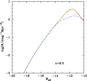
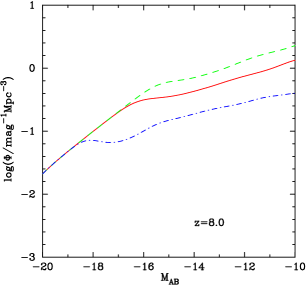
Figure 4: Effect of reionization history on luminosity function at z=8.0. Solid, dashed and dot-dashed lines have $\tau=$ 0.073, 0.058 and 0.088 respectively. Left panel shows the average case. Right panel shows the overdense case.

2.3 Radiative feedback

As we argue in the next section, the luminosity function of galaxies in an overdense region could carry an enhanced signature of feedback. We therefore highlight our feedback model in this subsection.

Radiation from stars in the first galaxies is expected to ionize and heat the surrounding medium. This increases the mass scale above which baryons can collapse in haloes. Also, as a result, the minimum mass of haloes that are able to cool is much higher in ionized regions than in the neutral ones. In our calculations, feedback appears through the quantity $M_{\mathrm{min}}(z)$ in Equation 4. The temperature evolution of both regions is calculated self-consistently. In the ionized regions, we fix the cut-off mass to that corresponding to a virial temperature of $10^{4}$ K or the local Jeans mass, whichever is higher. In the neutral regions, since the Jeans mass is always low, the cut-off mass always corresponds to the virial temperature of $10^{4}$ K. The minimum mass corresponds to the circular velocity of

$$v_{c}^{2}=\frac{2k_{\mathrm{boltz}}T}{\mu m_{p}},$$ (18)

where $\mu$ is the mean molecular weight. For a temperature of $\approx 10^{4}$ K, the minimum circular velocity is $\approx 25$ km s^-1. Note that this value is comparable to values obtained in simulations (Gnedin, 2000) but is somewhat higher than that taken in the semi-analytic prescription of Samui et al. (2007).

We find that $M_{\mathrm{min}}(z)$ increases with time taking values of $\approx 10^{7}$ M_⊙ at $z\approx 10$ and $\approx 10^{8}$ M_⊙ at $z\approx 7$. In overdense regions the minimum mass is enhanced to about $10^{10}$ M_⊙. Figure 5 shows the evolution of the minimum mass.

3 Results

The results for reionization and thermal histories within overdense regions are presented in this section.

Figure 5: Evolution of the minimum mass $M_{\mathrm{min}}(z)$ of haloes that can host galaxies in ionized regions in the average case (dashed line) and the overdense case (solid line). The dot-dashed line shows the minimum mass in neutral regions, which is same for the average and overdense cases.

3.1 Effect of overdensity on reionization history

We first consider the effect of overdensity on reionization history for our fiducial model. As is well known, reionization proceeds differently in overdense regions. The solid lines in Figure 1 show the evolution of the photoionisation rate, temperature in ionised regions, star formation rate density and the volume filling factor of ionised regions in an overdense region with size $R_{L}=1.482$ Mpc and linearly extrapolated overdensity $\delta=8.86$. This corresponds to the HUDF WFC3/IR field centred at the brightest source in Bouwens et al. (2010). (See Section 2.2.) Clearly while the average region is completely ionised at $z\approx 6$, the biased region is ionised much earlier, at $z\approx 7.5$. This result agrees with Wyithe & Loeb (2007), although note that unlike that work, here we calculate the clumping factor from a physical model for inhomogeneities. The reason for early reionization in overdense regions is the enhanced number of sources, which is clear from the plots of photoionisation rate and the star-formation rate, both of which are $\sim 5$ times higher than the corresponding globally averaged values. However, these overdense regions have more recombinations, which results in enhanced temperatures as is clear from the top right panel. This results in enhanced negative radiative feedback which will suppress star formation in low mass galaxies and hence affect the shape of the luminosity function. In fact, for the average case, haloes in ionised regions with masses below $10^{8}$ M_⊙ cannot form stars, whereas this cutoff mass rises to close to $10^{10}$ M_⊙ in the overdense case. Clearly feedback is enhanced in overdense regions.

3.2 Effect of overdensity on luminosity function

We now discuss the effect of overdensity on luminosity function. Clearly, overdense regions have enhanced number of sources, hence it is natural that the amplitude of the luminosity function for such regions should be higher than the globally averaged values. However, the overdense regions have enhanced radiative feedback too, and hence we expect a decrease in the number of sources, particularly towards the fainter end.

Figure 3 shows the effect of overdensity on the luminosity function at $z=8$ for our fiducial model. The ionised volume filling factor within the overdense region is $Q\approx 1.0$ for the overdense region under consideration at this redshift. The average region luminosity function (dashed line) is clearly very different from the luminosity function in the overdense region (solid line) at that redshift. Firstly, we can clearly see an enhancement in the source counts for brighter galaxies, which is as expected. In addition, there is a clear sign of a flattening for magnitudes $M_{\rm AB}\gtrsim-17$, which is a signature of radiative feedback. In comparison, the effect of feedback for average regions occurs at much fainter magnitudes $M_{\rm AB}\sim-12$. Note that there is no complete suppression of star formation for halo masses lower than the feedback threshold, rather the luminosity function for magnitudes below the knee continues to grow in the flattened region. This is simply due to the continued star formation in haloes with mass less than the cutoff mass at $z=8.0$, but which collapsed at higher redshifts when the feedback threshold mass was lower. Thus, for instance, if star formation is allowed to happen in a halo for only for a fraction of the dynamical time [see equation (3)], the luminosity function will rise less steeply at the fainter end. For small enough star formation time scale, the luminosity function will show an abrupt cutoff. Of course, an abrupt cutoff is always seen at low enough luminosities, which are not shown in the figure here.

It is important to understand here that the data points in Figure 2 do not represent luminosity function of the overdense region. Instead, those data points represent the globally averaged luminosity function derived using a maximum likelihood procedure from the observed luminosity distribution of sources. In this procedure, a likelihood function is defined, which describes the step-wise shape of the luminosity function that is most likely given the observed luminosity distribution in the search fields. Details of this procedure are described, for example, in Section 5.1 of Bouwens et al. (2010) and references therein.

3.3 Luminosity function as a probe of reionization

Given the fact that the effect of radiative feedback shows up at brighter magnitudes for overdense regions, it is possible to use this feature for studying feedback using near-future observations. For this purpose, we consider two additional models (other than the fiducial one) of reionization. These models have parameter values ($f_{*}$, $f_{\rm esc}$) = ($0.06$, $0.3$) and ($0.2,0.07$) and we obtain $\tau_{e}=0.088$ and $0.058$ respectively for these models. We fix $f_{*}$ and only change the value of $f_{\rm esc}$ to ensure that any effect on the luminosity function is purely due to feedback. These two models predict photoionisation rates greater and lesser respectively than what are presented by Bolton & Haehnelt (2007).

The right panel of Figure 4 shows the luminosity function at $z=8$ within the overdense region for three different reionization histories, which can be compared with the corresponding luminosity function in average region (shown in the left panel). In both cases a distinct “knee” is seen in the luminosity function as a signature of feedback. The luminosity function flattens at this luminosity, and is suppressed to very low values at much lower luminosities. As described in the previous section, this signature of feedback appears at brighter magnitudes for the overdense region. This is expected, because the cutoff mass depends directly on the temperature, which is enhanced in the overdense region. We also note that in the case of the first model the flattening occurs for $M_{\rm AB}\gtrsim-19$ whereas for the second model at a fainter luminosity of $M_{\rm AB}\simeq-16$. This is due to the fact that the photoionisation feedback is enhanced in the first model due to enhanced flux.

The evolution of the filling factor affects this result through the average temperature which sets the cutoff mass. Thus, early and late reionization models are distinguished by the difference in the nature of flattening in both cases. This also affects the evolution of the luminosity function.

We find that the reionization history has a strong effect on the luminosity function at the faint end. It is known that the bright end of the luminosity function is affected primarily by the star formation mode of a halo, and the overall bias, whereas its faint end is affected by the reionization history.

However, we also find, from Figure 4, that the effect of reionization history is much stronger in the case of overdense regions. This is because of the enhanced photoionisation feedback, which is more sensitive to changes in reionization history. This order of magnitude change in the overdense region luminosity function should be visible to the James Webb Space Telescope, which can observe up to $m_{\rm AB}\approx 31.5$ ($M_{\rm AB}\approx-16.0$ at redshifts of interest; Windhorst et al. 2006).

4 Discussion and Summary

We have used a semi-analytic model, based on Choudhury & Ferrara (2005, 2006) to study reionization and thermal history of an overdense region. Studying such regions is important because observations of galaxy luminosity function at high redshifts typically focus fields of view of limited sizes preferentially containing bright sources; these regions possibly are overdense and hence biased with respect to the globally averaged regions. In particular, we study the effect of radiative feedback arising from reionization on the shape of galaxy luminosity function.

In summary, we find that

1. Reionization proceeds differently in overdense regions. Overdense regions are ionised earlier because of enhanced number of sources and star formation. In addition, these regions have higher temperatures because of enhanced recombinations and hence effect of radiative feedback is enhanced too.

2. In particular, the shape of the galaxy luminosity function for biased regions is very different from that for average regions. There is a significant enhancement in the number of high-mass galaxies because of bias, while there is a reduction in low-mass galaxies resulting from enhanced radiative feedback.

3. Luminosity function in overdense regions is more sensitive to reionization history compared to average regions. The effect of radiative feedback shows up at absolute AB magnitudes $M_{\rm AB}\gtrsim-17$ in these regions, while it occurs at much fainter magnitudes $M_{\rm AB}\sim-12$ for average regions. This order of magnitude change in the overdense region luminosity function should be visible to the James Webb Space Telescope in future.

Finally, we critically examine some of the simplifying assumptions made in this work and how they are likely to affect our conclusions. Firstly, we have seen that the presence of a high mass galaxy within a region if size $R$ does not uniquely specify the value of the overdensity $\delta$. Rather we obtain a probability density (which is Gaussian in shape) and work with the value where this probability is maximum. In reality, however, the actual value of $\delta$ could be different and this may possibly affect the predicted luminosity function. Note that the luminosity function at the brighter end is almost independent of the details of reionization history, and this, in principle, can be used for constraining the value of $\delta$. The effect of feedback can then be studied using the faint end of the luminosity function.

The radiative feedback prescription used in this paper is based on a Jeans mass calculation (Choudhury & Ferrara, 2005). However, alternate prescriptions for feedback exist in literature, e.g., Gnedin (2000) and hence the shape of the luminosity function at faint ends as predicted by our model may not be robust. Interestingly, the presence of a “knee” in the luminosity function can be used to estimate the value of the halo mass below which star formation can be suppressed (which in turn can indicate the temperature) while the shape of the function below this knee should indicate the nature of feedback. This study can also be complemented with proposed for studying feedback using other observations, e.g., 21 cm observation (Schneider et al., 2008) and CMBR (Burigana et al., 2008).

Finally, we have neglected the presence of other sources of reionization, e.g., metal-free stars, minihaloes, and so on. It is expected that these sources would be too faint to affect the luminosity function in the ranges we are considering. However, these sources may affect the thermal history of the medium, e.g, the metal-free stars would produce higher temperatures because of harder spectra. In such cases, it is most likely that feedback would occur at magnitude brighter than what we have indicated and hence would possibly be easier to detect.

Appendix: Formation rate and survival probability of haloes in overdense regions

As expressed in Equation (5), the number density of ionizing photons produced per unit time is related to the SFR density, which in turn depends on the SFR in each halo, given by Equation (4), and the number density of haloes of a certain age, given by Equation (1) for average regions, and by Equation (15) for overdense regions. We derive Equation (15) in this appendix.

We denote the number density at redshift $z$ of haloes formed between redshifts $z_{c}$ and $z_{c}+dz_{c}$, with mass between $M$ and $M+dM$, by $N(M,z,z_{c})dMdz_{c}$. This quantity is related to (1) the formation rate at redshift $z_{c}$ of haloes with mass between $M$ and $M+dM$, denoted by $\dot{N}_{\mathrm{form}}(M,z_{c})dM$, and (2) the probability of their survival at redshift $z$, denoted by $p_{\mathrm{surv}}(z,z_{c})$. We calculate these two quantities using a technique given by Sasaki (1994), applied to an overdense region with overdensity $\delta$ and size $R$.

Recall that in extended Press-Schechter theory (Bond et al., 1991), the mass function of dark matter haloes is defined as the comoving number density of haloes with mass between $M$ and $M+dM$. At redshift $z$, this quantity is given by

$$N(M,z)dM=\sqrt{\frac{2}{\pi}}\frac{\bar{\rho}_{m}}{M}\exp\left(\frac{-\nu^{2}}{2}\right)\frac{d\nu}{dM}dM,$$ (19)

where $\bar{\rho}_{m}$ is the average matter density, and, as before, $\nu(M,z)\equiv\delta_{c}/[D(z)\sigma(M)]$. The critical overdensity of collapse of a halo is denoted by $\delta_{c}$, $D(z)$ is the growth function of density perturbations, and $\sigma(M)$ is the rms value of density perturbations at the comoving scale corresponding to mass $M$. In a region with overdensity $\delta$ and linear size $R$, the mass function is enhanced. This enhancement can be calculated using the excursion set formalism (Bond et al., 1991). The resulting mass function is again given by Equation (19), except that now the quantity $\nu(M,z)$ is defined as

$$\nu(M,z)\equiv\frac{\delta_{c}/D(z)-\delta}{\sqrt{\sigma^{2}(M)-\sigma^{2}_{R}}},$$ (20)

where $\sigma_{R}$ is the rms value of density perturbations at comoving scale $R$. Closely following Sasaki (1994), we can write

$$\dot{N}(M,z)=\dot{N}_{\mathrm{form}}(M,z)-\dot{N}_{\mathrm{dest}}(M,z),$$ (21)

where $\dot{N}_{\mathrm{dest}}(M,z)dM$ is the destruction rate at redshift $z$ of haloes of mass between $M$ and $dM$. (The halo formation rate is defined as the number density of haloes formed per unit time from mergers of lower mass haloes. Similarly the halo destruction rate is defined as the number density of haloes destroyed per unit time due to mergers with other haloes.) Here, an overdot denotes the time derivative. We can write the destruction rate as

$$\dot{N}_{\mathrm{dest}}(M,z) = \int_{M}^{\infty}N(M,z)\tilde{Q}(M,M^{\prime},z)dM^{\prime},$$ (22)

$$\equiv \phi(M,z)N(M,z),$$ (23)

and the formation rate as

$$\dot{N}_{\mathrm{form}}(M,z)=\int_{M_{\mathrm{min}}}^{M}N(M^{\prime},z)Q(M^{\prime},M,z)dM^{\prime},\\$$ (24)

where $\tilde{Q}(M,M^{\prime},z)$ is the probability that a halo of mass $M$ merges with another halo to result in a halo of mass $M^{\prime}$ per unit time, and $Q(M^{\prime},M,z)$ that an halo of mass $M$ forming at redshift $z$ has a progenitor of mass $M^{\prime}$. The threshold mass $M_{\mathrm{min}}$ is introduced at this stage to avoid divergence. This gives

$$\dot{N}_{\mathrm{form}}(M,z)=\dot{N}(M,z)+\phi(M,z)N(M,z).$$ (25)

We now assume that $\phi$ has no characteristic mass scale so that $\phi(M,z)=M^{\alpha}\tilde{\phi}(z)$. This gives

$$\tilde{\phi}(z)=\frac{-\dot{N}(M,z)+\dot{N}_{\mathrm{form}}(M,z)}{N(M,z)M^{\alpha}}.$$ (26)

But since the left hand side of Equation (26) is a function of time alone (through the redshift), the right hand side of this equation also has to be independent of mass. In particular, we can then set $M=M_{\mathrm{min}}$ in this equation, giving us

$$\tilde{\phi}(z)=\frac{-\dot{N}(M_{\mathrm{min}},z)}{N(M_{\mathrm{min}},z)M_{\mathrm{min}}^{\alpha}}.$$ (27)

Now, in the case of the overdense region that we are considering here, we have

$$\dot{N}(M,z)=N(M,z)\frac{\dot{D}(z)}{D^{2}(z)}\frac{\delta_{c}}{\delta_{c}/D(z)-\delta}[\nu^{2}(m,z)-1],$$ (28)

which gives

$$\tilde{\phi}=\frac{\dot{D}}{D^{2}}\frac{\delta_{c}}{\delta_{c}/D(z)-\delta}[\nu^{2}(M_{\mathrm{min}},z)-1]M_{\mathrm{min}}^{-\alpha}.$$ (29)

Since our choice of threshold mass $M_{\mathrm{min}}$ is arbitrary, we now need to take the limit $M_{\mathrm{min}}\rightarrow 0$. However, since $\nu\rightarrow 0$ in this limit, $\tilde{\phi}$ becomes indeterminate, except when $\alpha=0$. This implies that we must set $\alpha=0$ for consistency. This gives $\phi(M,z)=\tilde{\phi}(z)$. Substituting the resultant expression in Equation (25), we get

$$\dot{N}_{\mathrm{form}}(M,z)=N(M,z)\frac{\dot{D}}{D^{2}}\frac{\delta_{c}}{\delta_{c}/D(z)-\delta}\nu^{2}(M,z).$$ (30)

This the required formation rate of haloes in an overdense region.

Furthermore, from our definitions of probabilities in Equations (23) and (24), we can write the probability that a halo that has formed at redshift $z_{c}$ continues to exist at redshift $z$ as

$$p_{\mathrm{surv}}(z,z_{c})=\exp\left[-\int_{t(z_{c})}^{t(z)}\phi(t^{\prime})dt^{\prime}\right],$$ (31)

which in our case results in

$$p_{\mathrm{surv}}(z,z_{c})=\frac{\delta_{c}/D(z)-\delta}{\delta_{c}/D(z_{c})-\delta}.$$ (32)

From Equations (30) and (32), we can now write the the comoving number density $N(M,z,z_{c})dMdz_{c}$ at redshift $z$ of collapsed halos having mass in the range $M$ and $M+dM$ and redshift of collapse in the range $z_{c}$ and $z_{c}+dz_{c}$ as

$$\begin{split}N(M,z,z_{c})dMdz_{c}=N(&M,z_{c})\left(\frac{\nu^{2}\delta_{c}}{\delta_{c}/D(z_{c})-\delta}\right)\frac{\dot{D}(z_{c})}{D^{2}(z_{c})}\\ &\times p_{\mathrm{surv}}(z,z_{c})\frac{dt}{dz_{c}}dz_{c}dM,\end{split}$$ (33)

This is our Equation (15).

It is worth pointing out that Equations (30) and (32) reduce to the average forms for halo formation rate and survival probability in the limit $\delta\rightarrow 0$ and $R\rightarrow\infty$.

References

- Bolton & Haehnelt (2007) Bolton J. S., Haehnelt M. G., 2007, MNRAS, 382, 325
- Bond et al. (1991) Bond J. R., Cole S., Efstathiou G., Kaiser N., 1991, ApJ, 379, 440
- Bouwens & Illingworth (2006) Bouwens R., Illingworth G., 2006, New Astronomy Review, 50, 152
- Bouwens et al. (2009) Bouwens R. J., Illingworth G. D., Franx M., Chary R., Meurer G. R., Conselice C. J., Ford H., Giavalisco M., van Dokkum P., 2009, ApJ, 705, 936
- Bouwens et al. (2007) Bouwens R. J., Illingworth G. D., Franx M., Ford H., 2007, ApJ, 670, 928
- Bouwens et al. (2008) Bouwens R. J., Illingworth G. D., Franx M., Ford H., 2008, ApJ, 686, 230
- Bouwens et al. (2010) Bouwens R. J., Illingworth G. D., Gonzalez V., Labbe I., Franx M., Conselice C. J., Blakeslee J., van Dokkum P., Ford H., Holden B., Marchesini D., Magee D., Zheng W., 2010, ArXiv e-prints
- Bouwens et al. (2009) Bouwens R. J., Illingworth G. D., Labbe I., Oesch P. A., Carollo M., Trenti M., van Dokkum P. G., Franx M., Stiavelli M., Gonzalez V., Magee D., 2009, ArXiv e-prints
- Bouwens et al. (2010) Bouwens R. J., Illingworth G. D., Oesch P. A., Labbe I., Trenti M., van Dokkum P., Franx M., Stiavelli M., Carollo C. M., Magee D., Gonzalez V., 2010, ArXiv e-prints
- Bouwens et al. (2010) Bouwens R. J., Illingworth G. D., Oesch P. A., Stiavelli M., van Dokkum P., Trenti M., Magee D., Labbé I., Franx M., Carollo C. M., Gonzalez V., 2010, ApJ, 709, L133
- Bouwens et al. (2010) Bouwens R. J., Illingworth G. D., Oesch P. A., Trenti M., Stiavelli M., Carollo C. M., Franx M., van Dokkum P. G., Labbé I., Magee D., 2010, ApJ, 708, L69
- Bradley et al. (2008) Bradley L. D., Bouwens R. J., Ford H. C., Illingworth G. D., Jee M. J., Benítez N., Broadhurst T. J., Franx M., Frye B. L., Infante L., Motta V., Rosati P., White R. L., Zheng W., 2008, ApJ, 678, 647
- Bunker et al. (2009) Bunker A., Wilkins S., Ellis R., Stark D., Lorenzoni S., Chiu K., Lacy M., Jarvis M., Hickey S., 2009, ArXiv e-prints
- Bunker et al. (2010) Bunker A. J., Wilkins S., Ellis R. S., Stark D. P., Lorenzoni S., Chiu K., Lacy M., Jarvis M. J., Hickey S., 2010, MNRAS, pp 1378–+
- Burigana et al. (2008) Burigana C., Popa L. A., Salvaterra R., Schneider R., Choudhury T. R., Ferrara A., 2008, MNRAS, 385, 404
- Castellano et al. (2010) Castellano M., Fontana A., Boutsia K., Grazian A., Pentericci L., Bouwens R., Dickinson M., Giavalisco M., Santini P., Cristiani S., Fiore F., Gallozzi S., Giallongo E., Maiolino R., Mannucci F., and others 2010, A&A, 511, A20+
- Cen (2005) Cen R., 2005, ArXiv Astrophysics e-prints
- Cen et al. (2005) Cen R., Haiman Z., Mesinger A., 2005, ApJ, 621, 89
- Choudhury & Ferrara (2005) Choudhury T. R., Ferrara A., 2005, MNRAS, 361, 577
- Choudhury & Ferrara (2006) Choudhury T. R., Ferrara A., 2006, MNRAS, 371, L55
- Choudhury et al. (2008) Choudhury T. R., Ferrara A., Gallerani S., 2008, MNRAS, 385, L58
- Cooray & Sheth (2002) Cooray A., Sheth R., 2002, Phys. Rep., 372, 1
- Dijkstra et al. (2007) Dijkstra M., Wyithe J. S. B., Haiman Z., 2007, MNRAS, 379, 253
- Fan et al. (2006) Fan X., Strauss M. A., Becker R. H., White R. L., Gunn J. E., Knapp G. R., Richards G. T., Schneider D. P., Brinkmann J., Fukugita M., 2006, AJ, 132, 117
- Finkelstein et al. (2010) Finkelstein S. L., Papovich C., Giavalisco M., Reddy N. A., Ferguson H. C., Koekemoer A. M., Dickinson M., 2010, ApJ, 719, 1250
- Gallerani et al. (2008a) Gallerani S., Ferrara A., Fan X., Choudhury T. R., 2008a, MNRAS, 386, 359
- Gallerani et al. (2008b) Gallerani S., Salvaterra R., Ferrara A., Choudhury T. R., 2008b, MNRAS, 388, L84
- Geil & Wyithe (2009) Geil P. M., Wyithe J. S. B., 2009, MNRAS, 399, 1877
- Gnedin (2000) Gnedin N. Y., 2000, ApJ, 542, 535
- Gunn & Peterson (1965) Gunn J. E., Peterson B. A., 1965, ApJ, 142, 1633
- Haiman & Cen (2005) Haiman Z., Cen R., 2005, ApJ, 623, 627
- Henry et al. (2008) Henry A. L., Malkan M. A., Colbert J. W., Siana B., Teplitz H. I., McCarthy P., 2008, ApJ, 680, L97
- Henry et al. (2007) Henry A. L., Malkan M. A., Colbert J. W., Siana B., Teplitz H. I., McCarthy P., Yan L., 2007, ApJ, 656, L1
- Henry et al. (2009) Henry A. L., Siana B., Malkan M. A., Ashby M. L. N., Bridge C. R., Chary R., Colbert J. W., Giavalisco M., Teplitz H. I., McCarthy P. J., 2009, ApJ, 697, 1128
- Hickey et al. (2010) Hickey S., Bunker A., Jarvis M. J., Chiu K., Bonfield D., 2010, MNRAS, 404, 212
- Iliev et al. (2008) Iliev I. T., Shapiro P. R., McDonald P., Mellema G., Pen U., 2008, MNRAS, 391, 63
- Iye et al. (2006) Iye M., Ota K., Kashikawa N., Furusawa H., Hashimoto T., Hattori T., Matsuda Y., Morokuma T., Ouchi M., Shimasaku K., 2006, Nature, 443, 186
- Kim et al. (2009) Kim S., Stiavelli M., Trenti M., Pavlovsky C. M., Djorgovski S. G., Scarlata C., Stern D., Mahabal A., Thompson D., Dickinson M., Panagia N., Meylan G., 2009, ApJ, 695, 809
- Larson et al. (2010) Larson D., Dunkley J., Hinshaw G., Komatsu E., Nolta M. R., Bennett C. L., Gold B., Halpern M., Hill R. S., Jarosik N., Kogut A., Limon M., Meyer S. S., Odegard N., Page L., 2010, ArXiv e-prints
- Leitherer et al. (1999) Leitherer C., Schaerer D., Goldader J. D., González Delgado R. M., Robert C., Kune D. F., de Mello D. F., Devost D., Heckman T. M., 1999, ApJS, 123, 3
- McLure et al. (2009) McLure R. J., Cirasuolo M., Dunlop J. S., Foucaud S., Almaini O., 2009, MNRAS, 395, 2196
- McLure et al. (2010) McLure R. J., Dunlop J. S., Cirasuolo M., Koekemoer A. M., Sabbi E., Stark D. P., Targett T. A., Ellis R. S., 2010, MNRAS, 403, 960
- Miralda-Escudé et al. (2000) Miralda-Escudé J., Haehnelt M., Rees M. J., 2000, ApJ, 530, 1
- Muñoz & Loeb (2008) Muñoz J. A., Loeb A., 2008, MNRAS, 385, 2175
- Oesch et al. (2010) Oesch P. A., Bouwens R. J., Illingworth G. D., Carollo C. M., Franx M., Labbé I., Magee D., Stiavelli M., Trenti M., van Dokkum P. G., 2010, ApJ, 709, L16
- Oesch et al. (2009) Oesch P. A., Carollo C. M., Stiavelli M., Trenti M., Bergeron L. E., Koekemoer A. M., Lucas R. A., Pavlovsky C. M., Beckwith S. V. W., Dahlen T., Ferguson H. C., Gardner J. P., Lilly S. J., Mobasher B., Panagia N., 2009, ApJ, 690, 1350
- Oke & Gunn (1983) Oke J. B., Gunn J. E., 1983, ApJ, 266, 713
- Ota et al. (2008) Ota K., Iye M., Kashikawa N., Shimasaku K., Kobayashi M., Totani T., Nagashima M., Morokuma T., Furusawa H., Hattori T., Matsuda Y., Hashimoto T., Ouchi M., 2008, ApJ, 677, 12
- Ouchi et al. (2009) Ouchi M., Mobasher B., Shimasaku K., Ferguson H. C., Fall S. M., Ono Y., Kashikawa N., Morokuma T., Nakajima K., Okamura S., Dickinson M., Giavalisco M., Ohta K., 2009, ApJ, 706, 1136
- Ouchi et al. (2009) Ouchi M., Ono Y., Egami E., Saito T., Oguri M., McCarthy P. J., Farrah D., Kashikawa N., Momcheva I., Shimasaku K., Nakanishi K., Furusawa H., Akiyama M., Dunlop J. S., and others 2009, ApJ, 696, 1164
- Press & Schechter (1974) Press W. H., Schechter P., 1974, ApJ, 187, 425
- Pritchard & Furlanetto (2007) Pritchard J. R., Furlanetto S. R., 2007, MNRAS, 376, 1680
- Richard et al. (2008) Richard J., Stark D. P., Ellis R. S., George M. R., Egami E., Kneib J., Smith G. P., 2008, ApJ, 685, 705
- Samui et al. (2007) Samui S., Srianand R., Subramanian K., 2007, MNRAS, 377, 285
- Samui et al. (2009) Samui S., Srianand R., Subramanian K., 2009, MNRAS, 398, 2061
- Sasaki (1994) Sasaki S., 1994, PASJ, 46, 427
- Schneider et al. (2008) Schneider R., Salvaterra R., Choudhury T. R., Ferrara A., Burigana C., Popa L. A., 2008, MNRAS, 384, 1525
- Sobral et al. (2009) Sobral D., Best P. N., Geach J. E., Smail I., Kurk J., Cirasuolo M., Casali M., Ivison R. J., Coppin K., Dalton G. B., 2009, MNRAS, 398, L68
- Stark et al. (2007) Stark D. P., Ellis R. S., Richard J., Kneib J., Smith G. P., Santos M. R., 2007, ApJ, 663, 10
- Thoul & Weinberg (1996) Thoul A. A., Weinberg D. H., 1996, ApJ, 465, 608
- Vale & Ostriker (2004) Vale A., Ostriker J. P., 2004, MNRAS, 353, 189
- Vázquez & Leitherer (2005) Vázquez G. A., Leitherer C., 2005, ApJ, 621, 695
- Windhorst et al. (2006) Windhorst R. A., Jansen R. A., Cohen S. H., Mechtley M., Yan H., Conselice C., 2006, in Bulletin of the American Astronomical Society Vol. 38 of Bulletin of the American Astronomical Society, How can the James Webb Space Telescope measure First Light, Reionization, and Galaxy Assembly?. pp 1188–+
- Wyithe et al. (2008) Wyithe J. S. B., Bolton J. S., Haehnelt M. G., 2008, MNRAS, 383, 691
- Wyithe & Loeb (2005) Wyithe J. S. B., Loeb A., 2005, ApJ, 625, 1
- Wyithe & Loeb (2007) Wyithe J. S. B., Loeb A., 2007, MNRAS, 375, 1034
- Zheng et al. (2009) Zheng W., Bradley L. D., Bouwens R. J., Ford H. C., Illingworth G. D., Benítez N., Broadhurst T., Frye B., Infante L., Jee M. J., Motta V., Shu X. W., Zitrin A., 2009, ApJ, 697, 1907