A source-free integration method for black hole perturbations
and self-force computation: radial fall

Abstract

Perturbations of Schwarzschild-Droste black holes in the Regge-Wheeler gauge benefit from the availability of a wave equation and from the gauge invariance of the wave function, but lack smoothness. Nevertheless, the even perturbations belong to the C⁰ continuity class, if the wave function and its derivatives satisfy specific conditions on the discontinuities, known as jump conditions, at the particle position. These conditions suggest a new way for dealing with finite element integration in the time domain. The forward time value in the upper node of the $(t,r^{*}$) grid cell is obtained by the linear combination of the three preceding node values and of analytic expressions based on the jump conditions. The numerical integration does not deal directly with the source term, the associated singularities and the potential. This amounts to an indirect integration of the wave equation. The known wave forms at infinity are recovered and the wave function at the particle position is shown. In this series of papers, the radial trajectory is dealt with first, being this method of integration applicable to generic orbits of EMRI (Extreme Mass Ratio Inspiral).

I Introduction

It is currently affirmed that the core of most galaxies host supermassive black holes, on which stars and compact objects in the neighbourhood inspiral and plunge-in. The EMRI (Extreme Mass Ratio Inspiral) sources are characterised by a huge number of parameters that, when spanned over a large period, produce a huge number of templates for the LISA (Laser Interferometer Space Antenna) project li . Thus, matched filtering (the superposition of the expected and received signals)sasc03 is aided by stochastic methods po09 ; in alternative, other more robust methods based on covariance or on time and frequency analysis are investigated sasc03 ; gajo07 ; gamawe08a ; gamawe08b ; co10 ; bagapo09 . Furthermore, if the signal from a capture is not individually detectable, it still may contribute to the statistical background bacu04 ; racu07 . Detection strategies are to be tested by the LISA simulators coru03 ; va05 ; peauhajeplpirevi08 .

Challenges by EMRIs arise increasing interest amongst astrophysicists and those studying data analysis, but also for theorists. Relativists, especially, have been drawn to study EMRIs for the determination of the motion of the captured mass and because of the impact that back-action has on the gravitational wave forms (see blspwh10 where a comprehensive introduction to these topics is given).

The captured compact object may be compared to a small mass $m$ perturbing the background spacetime curvature of a large mass $M$ and generating gravitational radiation. Perturbation methods from the seminal work of Regge and Wheeler, henceforth RW rewh57 , were an obvious aid for studying the case we are dealing with. Approaches based on numerical relativity (NR) appear not be best suited, nor do the post-Newtonian (pN) expansions: the former for the two-scale problem (one small scale for the neighbourhood of the particle, one large scale for the radiation at infinity); the latter for the small field and low velocity constraints. To EMRIs, nevertheless, Damour, Nagar and co-workers nadata07 ; dana07 ; bena10 ; da09b , and Yunes et al. yubuhumipa10 have applied the EOB (effective one body) method, though based on the pN approach. Furthermore, both pN and perturbation methods are found to be in agreement in their common domain of applicability by Blanchet et al. bldeltwh10a ; bldeltwh10b , as well as EOB and perturbation methods have shown their synergy thanks to Barack et al. badasa10 . Finally, it is to be mentioned that NR analysis is slowly progressing towards unequal mass ratios sp10 .

I.1 Perturbation methods

EMRIs have revived the interest for the perturbative relativistic two-body problem, which was investigated with a semi-relativistic approach some 40 years ago by Ruffini and Wheeler ruwh71a ; ruwh71b , and then more fully by Zerilli ze69 ; ze70a ; ze70b ; ze70c . These authors treated the source of the perturbations in the form of a radially falling particle. Zerilli’s results opened the way for others to study to first order the orbital motion of the captured mass in a fully, although linearised, relativistic regime. Work done up until the end of the ’90s involved the captured star moving on the geodesic of the background field and being unaffected by its own mass and the emitted radiation.

We shall refer to the first solution of the Einstein equation as the work of Droste dr15 ; dr16a ; dr16b and Schwarzschild sc16 , collectively as SD, this double authorship having been justified by the historians, as recalled by Rothman ro02 . Much research has been devoted to the study of SD black hole perturbations in the RW gauge, first in a vacuum rewh57 , and then by Zerilli in the presence of a source ze69 ; ze70a ; ze70b ; ze70c . An outflow of publications by Davis, Press, Price, Ruffini and Tiomno daruprpr71 ; daru72 ; daruti72 ; ru73a ; ru73b ; ru78 , but also by individual scholars like Chung ch73 , Dymnikova dy80 appeared in the ’70s. It was followed by a slowdown in the ’80s and ’90s, with the exception of the forerunners of the Japanese school as Tashiro and Ezawa taez81 , Nakamura with Oohara and Koijma naooko87 or with Shibata shna92 . The aim of all these authors was to analyse especially the amplitude and spectrum of the radiation emitted by the falling mass. Simulations were performed in frequency domain with the particle falling from infinity. The numerical accuracy was recently improved by Mitsou mi10 . It was in 1997, that a fall from finite distance was analysed by Lousto and Price lopr97a . The latter two authors were the first to use a finite difference scheme in time domain lopr97b . Following on this work, Martel and Poisson mapo02 were able to parametrise the initial conditions reflecting past motion of the particle and resulting into an initial amount of gravitational wave energy. All of this work was carried out in the RW gauge.

It is less than 15 years since we began to have methods for evaluating the back-action for point masses in strong fields thanks to two concurring situations. On one hand, the theorists progressed in understanding radiation reaction and obtained formal prescriptions for its determination. The solution was brought by the self-force equation, first by Mino, Sasaki and Tanaka misata97 , Quinn and Wald quwa97 , and later by Detweiler and Whiting dewh03 , all various approaches yielding the same formal expression. On the other hand, for the above mentioned detection of captures, the requirements from LISA posed constraints on the tolerable amount of phase-shift on the wave forms, caused by radiation reaction. This impulse - project oriented - compelled the researchers to turn their efforts in finding an efficient and clear implementation of the prescription made by the theorists. The development was again pursued in perturbation theory. This time, though, the small mass $m$ is correcting the geodesic equation of motion on a fixed background via a factor ${\cal O}(m)$.

Actually, the advances in the field by e.g. Warburton and Barack waba10 and in radiation gauge by Keidl et al. KeShFrKiPr10 have recently tackled the self-force in Kerr geometry ke63 . Such initial results in Kerr geometry do not mean that all major issues in non-rotating black holes have been solved. For instance, the self-consistent evolution of an orbit, along the lines suggested by Gralla and Wald grwa08 , is not yet applied even to the simpler case of non-rotating black holes.

I.2 A different integration approach

The complexity in assessing the continuity of the perturbations (and the associated numerical computation of derivatives) at the position of the particle, has led Barack and Lousto balo05 , among other motivations such as the compatibility of the self-force to the (Lorenz-FitzGerald-de Donder) harmonic gauge lo67 ; hu91 ; dd21 , to convey their efforts to this gauge. This alternative enterprise is by no means priceless, the price being the unavailability of a wave equation like in the RW gauge and of the gauge invariance of the wave function, as determined by Moncrief mo74 . In this context, the recent investigations of a gauge independent form of the self-force gr10 may change sensibly the trade-off on the gauge choice.

The choice of a gauge should be suited to the type of problem under scrutiny and thus we do not adopt a position on which gauge should be preferred a priori. We find of some interest to revert a weakness of the RW gauge, namely the lack of smoothness, into a building tool of a new integration method.

Indeed, we propose herein a finite element method of integration based on the jump conditions that the wave function and its derivatives have to satisfy for the SD black hole perturbations to be continuous at the position of the particle. We first deal with the radial trajectory and the associated even parity perturbations, while in a forthcoming paper aosp11 we shall present the circular and eccentric orbital cases, referring thus to both odd and even parity perturbations.

Herein, we present a first order method and show that it suffices to acquire a well-behaved wave function at infinity and at the particle position. However, a higher order scheme has been derived and tested rispaoco11 .

The main feature of the indirect (-I-) method consists in avoiding the explicit integration of the wave equation (the source term with the associated singularities and the potential) whenever the grid cells are crossed by the particle. Indeed, the information on the wave equation is implicitly given by the jump conditions. Conversely, for cells not crossed by the particle, we retain the classic approach for integrating wave equations lopr97b ; mapo02 , henceforth named LPMP.

For the computation of the back-action, the -I- method ensures a well behaved wave function at the particle position, since the approach is governed by the theoretical values of the jump conditions.

I.3 Structure of the paper

The structure of the paper is as follows. Section II is a brief reminder of the formalism on perturbations for a SD black hole in the RW gauge. In Sec. III, we give an overview about the jump conditions on the wave function and its derivatives. In Sec. IV, we introduce the scheme by detailing one of the four physical cases that a particle crossing the mesh cell during its infall may encounter, while for the other three similar cases we simply provide the final result. In Sec. V some wave forms at infinity are shown, discussed and compared to those obtained with the LPMP method. Furthermore, the theoretical and numerical jump conditions at the position of the particle are displayed and commented. In the conclusions, Sec. VI, the perspectives are addressed.

Geometric units ($G=c=1$) are used, unless stated otherwise. The metric signature is $(-,+,+,+)$.

II Black hole perturbations

The Zerilli-Moncrief (ZM) equation rules even-parity waves in the presence of a source: a freely falling point particle, that generates a perturbation for which the difference from the SD geometry is small. The energy-momentum tensor $T_{\mu\nu}$ is given by the integral of the world line of the particle, the integrand containing a four-dimensional invariant $\delta$ Dirac distribution for the representation of the point particle trajectory. The vanishing of the covariant divergence of $T_{\mu\nu}$ is guaranteed by the world line being a geodesic in the background SD geometry, represented by the metric tensor $g_{\mu\nu}$. Finally, the complete description of the emitted gravitational waves is given by the symmetric tensor $h_{\mu\nu}\ll g_{\mu\nu}$.

The formalism can be summarised as follows. Any symmetric covariant tensor can be expanded in spherical harmonics ze70b . Because of the spherical symmetry of the SD field, the linearised field equations are cast in the form of a rotationally invariant operator on $h_{\mu\nu}$. This term is equated to the energy-momentum tensor, also expressed in spherical tensorial harmonics. That is:

$$Q[h_{\mu\nu}]\propto T_{\mu\nu}[\delta(r_{u})]~{}~{},$$ (1)

where the $\delta(r_{u})$ Dirac distribution represents the point particle unperturbed trajectory $r_{u}$. The rotational invariance is used to separate out the angular variables in the field equations. For the spherical symmetry of the 2-dimensional manifold on which $t,r$ are constants under rotation in the $\theta,\phi$ sphere, the ten components of the perturbing symmetric tensor transform like three scalars, two vectors and one tensor:

$$h_{tt},h_{tr},h_{rr}~{}~{}~{}~{}~{}~{}~{}~{}~{}~{}~{}(h_{t\theta};h_{t\phi}),(h_{r\theta};h_{r\phi})~{}~{}~{}~{}~{}~{}~{}~{}~{}~{}~{}\left(\begin{matrix}h_{\theta\theta}&h_{\theta\phi}\cr h_{\phi\theta}&h_{\phi\phi}\end{matrix}\right)~{}~{}.$$

In the Regge-Wheeler-Zerilli formalism, the source term for the odd perturbations vanishes for the radial trajectory and, given the rotational invariance through the azimuthal angle, only the index referring to the polar or latitude angle survives. The even perturbations, going as $(-1)^{l}$, are expressed by the following matrix:

$$h_{\mu\nu}=\left(\begin{matrix}\left(1-\frac{\displaystyle 2M}{\displaystyle r}\right)H^{l}_{0}Y^{l}&H^{l}_{1}Y^{l}&h^{l}_{0}Y^{l}_{,\theta}&h^{l}_{0}Y^{l}_{,\phi}\cr sym&\left(1-\frac{\displaystyle 2M}{\displaystyle r}\right)^{-1}H^{l}_{2}Y^{l}&h^{l}_{1}Y^{l}_{,\theta}&h^{l}_{1}Y^{l}_{,\phi}\cr sym&sym&r^{2}\left[K^{l}Y^{l}+G^{l}Y^{l}_{,\theta\theta}\right]&r^{2}G^{l}\left(Y^{l}_{,\theta\phi}-\cot\theta Y^{l}_{,\phi}\right)\cr sym&sym&sym&r^{2}\sin^{2}\theta\left[K^{l}+G^{l}\left(\frac{\displaystyle Y^{l}_{,\phi\phi}}{\displaystyle\sin^{2}\theta}+\cot\theta Y^{l}_{,\theta}\right)\right]\end{matrix}\right)~{}~{},$$ (2)

where $H^{l}_{0},H^{l}_{1},H^{l}_{2},h^{l}_{0},h^{l}_{1},K^{l},G^{l}$ are functions of $(t,r)$ and the spherical harmonics $Y^{l}$ obviously of $(\theta,\phi)$. Two formalisms describe the evolution of the perturbations in terms of a single wave function and a single wave equation. One, due to Moncrief mo74 , gauge invariant and developed about a 3-geometry of a t = constant hypersurface, refers solely to the $H^{l}_{2},K^{l},G^{l},h^{l}_{1},$ perturbations. The other, due to Zerilli ze69 ; ze70a ; ze70b ; ze70c , uses the RW gauge $G^{l}=h^{l}_{0}=h^{l}_{1}=0$. In the RW gauge, the Moncrief wave function is given by:

$$\Psi_{l}(t,r)=\frac{r}{\lambda+1}\left[K^{l}+\frac{r-2M}{\lambda r+3M}\left(H_{2}^{l}-r\frac{\partial K^{l}}{\partial r}\right)\right],$$ (3)

where the Zerilli ze70a normalisation is used for $\Psi_{l}$. The dimension of the wave function is such that the energy is proportional to $\int_{0}^{\infty}\dot{\Psi}^{2}\,dt$. Finally, the wave equation is given by:

$$\frac{\partial^{2}\Psi^{l}(t,r)}{\partial r^{*2}}-\frac{\partial^{2}\Psi^{l}(t,r)}{\partial t^{2}}-V^{l}(r)\Psi^{l}(t,r)=S^{l}(t,r)~{}~{},$$ (4)

where $r^{*}=r+2M\ln(r/2M-1)$ is the tortoise coordinate. The potential $V^{l}(r)$ is expressed by:

$$V^{l}(r)=\left(1-\frac{2M}{r}\right)\frac{2\lambda^{2}(\!\lambda\!+\!1\!)r^{3}\!\!+\!6\lambda^{2}Mr^{2}\!+\!18\lambda M^{2}r\!+\!18M^{3}}{r^{3}(\lambda r\!+\!3M)^{2}}~{}~{},$$ (5)

being $\lambda=1/2(l-1)(l+2)$. The source $S^{l}(t,r)$ includes the derivative of the Dirac distribution, which appears in the process of building a single wave equation out of the seven even linearised wave equations:

$$S^{l}=\frac{2(r-2M)\kappa}{r^{2}(\lambda+1)(\lambda r+3M)}\times\left\{\frac{r(r-2M)}{2U^{0}}\delta^{\prime}[r-r_{u}(t)]-\left[\frac{r(\lambda+1)-3M}{2U^{0}}-\frac{3MU^{0}(r-2M)^{2}}{r(\lambda r+3M)}\right]\delta[r-r_{u}(t)]\right\}~{}~{},$$ (6)

$U^{0}=\sqrt{1-2M/r_{u0}}/(1-2M/r_{u})$ being the time component of the 4-velocity and $\kappa=4m\sqrt{(2l+1)\pi}$. The trajectory in the unperturbed SD metric $r_{u}(t)$ assumes different forms according to the initial conditions. For the radial infall of a particle starting from rest at finite distance $r_{u0}$, $r_{u}(t)$ is the inverse function of:

$$\frac{t(r_{u})}{2M}=\sqrt{1-\frac{2M}{r_{u0}}}\sqrt{1-\frac{r_{u}}{r_{u0}}}\left(\frac{r_{u0}}{2M}\right)\left(\frac{r_{u}}{2M}\right)^{1/2}+2{\rm{arctanh}}\left(\frac{\sqrt{\displaystyle\frac{2M}{r_{u}}-\frac{2M}{r_{u0}}}}{\sqrt{\displaystyle 1-\frac{2M}{r_{u0}}}}\right)+$$

$$\sqrt{1-\frac{2M}{r_{u0}}}\left(1+\frac{4M}{r_{u0}}\right)\left(\frac{r_{u0}}{2M}\right)^{3/2}\arctan\left(\sqrt{\frac{r_{u0}}{r}-1}\right)$$ (7)

where $E=\sqrt{1-2M/r_{u0}}$.

For an infalling mass from infinity at zero velocity, the energy radiated to infinity for all modes daruprpr71 is given by (in physical units):

$$\sum_{l}E^{l}_{rad}=0.0104\frac{m^{2}c^{2}}{M}~{}~{},$$ (8)

while most of the energy is emitted below the frequency:

$$f_{m}=0.08\frac{c^{3}}{GM}~{}~{}.$$ (9)

Up to $94\%$ of the energy is radiated between $8M$ and $2M$ and $90\%$ of it in the quadrupole mode. Obviously the above expressions would sensibly vary in case of an initial relativistic velocity.

For the SD black hole perturbations, there have been successive corrections of the basic equations, the last being pointed out by Sago, Nakano and Sasaki sanasa03 . Sago et al. have corrected the ZM equations (a minus sign missing in all right-hand side terms) but introduced a wrong definition of the scalar product leading to errors in the coefficients of the energy-momentum tensor na10 . The expressions herein correspond to those in sp11 , where some of the errors of previously published literature on radial fall are indicated.

III The jump conditions

It has been indicated by two different heuristic arguments lo00 ; lona09 that even metric perturbations, for radial fall in the RW gauge, should belong to the $C^{0}$ continuity class at the position of the particle. One argument lo00 is based on the integration in $r$ of the Hamiltonian constraint, which is the $tt$ component of the Einstein equations (Eq. (C7a) in ze70c ); the other lona09 on the structure of selected even perturbation equations. Following the latter, Lousto and Nakano evince the continuity of the even perturbations and afterwards impose such continuity to derive the jump conditions on the wave function and its derivatives for $l=2$, notably starting from the ZM equation.

In this section, we instead provide an analysis vis à vis the jump conditions that the wave function and its derivatives have to satisfy for guaranteeing the continuity of the perturbations at the position of the particle. This approach aosp1011 is based on the solutions of the ZM equation, not on the equation itself. The jump conditions found herein are applicable to all modes. Incidentally, the jump conditions were previously mentioned by Sopuerta and Laguna sola06 , Haas ha07 , and Field et al. fihela09 in a different context. In the forthcoming paper aosp11 , the jump conditions for generic orbits are based on the analysis of the odd and even wave equations and are determined despite the lack of continuity of the perturbations.

In the radial case, only three independent perturbations survive, namely $K^{l}$, $H^{l}_{0}=H^{l}_{2}$, $H^{l}_{1}$. The inverse relations for those perturbations, as functions of the wave function and its derivatives, are given by (we drop henceforth the $l$ index):

$$K=\frac{6M^{2}+3M\lambda r+\lambda(\lambda+1)r^{2}}{r^{2}(\lambda r+3M)}\Psi+\left(1-\frac{2M}{r}\right)\,\Psi_{,r}-\frac{\kappa\ U^{0}(r-2M)^{2}}{(\lambda+1)(\lambda r+3M)r}\delta~{}~{},$$ (10)

$$H_{2}=-\frac{9M^{3}+9\lambda M^{2}r+3\lambda^{2}Mr^{2}+\lambda^{2}(\lambda+1)r^{3}}{r^{2}(\lambda r+3M)^{2}}\,\Psi+\frac{3M^{2}-\lambda Mr+\lambda r^{2}}{r(\lambda r+3M)}\Psi_{,r}+$$

$$(r-2M)\Psi_{,rr}+\frac{\kappa U^{0}(r-2M)(\lambda^{2}r^{2}+2\lambda Mr-3Mr+3M^{2})}{r(\lambda+1)(\lambda r+3M)^{2}}\delta-\frac{\kappa U^{0}(r-2M)^{2}}{(\lambda+1)(\lambda r+3M)}\delta^{\prime}~{}~{},$$ (11)

$$H_{1}=\frac{\lambda r^{2}-3M\lambda r-3M^{2}}{\left(r-2M\right)(\lambda r+3M)}{\Psi_{,t}}+r\Psi_{,tr}-\frac{\kappa\ U^{0}\stackrel{{\scriptstyle.}}{{z}}_{u}(\lambda r+M)}{(\lambda+1)(\lambda r+3M)}\delta+\frac{\kappa\ U^{0}\stackrel{{\scriptstyle.}}{{z}}_{u}r(r-2M)}{(\lambda+1)(\lambda r+3M)}\delta^{\prime}~{}~{},$$ (12)

where $\delta=\delta\left[r-r_{u}(t)\right]$ and $\delta^{\prime}=\delta^{\prime}\left[r-r_{u}(t)\right]$.

From the visual inspection of the ZM wave equation (4), it is evinced that the wave function $\Psi$ is of $C^{-1}$ continuity class, since the second derivative of the wave function is proportional to the first derivative of the Dirac distribution (incidentally, the concept of $C^{-1}$ continuity class element, like a Heaviside step distribution, may be pragmatically introduced as an element of a class of functions which after integration transforms into an element belonging to the $C^{0}$ class of functions). Thus, the wave function and its derivatives can be written as:

$$\Psi=\!\Psi^{+}(t,r)~{}\Theta_{1}+\Psi^{-}(t,r)~{}\Theta_{2}~{}~{},$$ (13)

$$\Psi_{,r}\!=\!\Psi^{+}_{,r}\Theta_{1}+\Psi^{-}_{,r}\Theta_{2}+\left(\Psi^{+}\!-\!\Psi^{-}\right)\delta~{}~{},$$ (14)

$$\Psi_{,rr}\!=\!\Psi^{+}_{,rr}\Theta_{1}\!+\!\Psi^{-}_{,rr}\Theta_{2}\!+\!\left(\Psi^{+}_{,r}\!-\!\Psi^{-}_{,r}\right)\delta\!+\!\left(\Psi^{+}\!-\!\Psi^{-}\right)_{r_{u}}\!\!\delta^{\prime}~{}~{},$$ (15)

$$\Psi_{,t}\!=\!\Psi^{+}_{,t}\Theta_{1}\!+\!\Psi^{-}_{,t}\Theta_{2}\!-\!\left(\Psi^{+}\!-\!\Psi^{-}\right)\dot{r}_{u}\delta~{}~{},$$ (16)

$$\Psi_{,tr}\!=\!\Psi^{+}_{,tr}\Theta_{1}\!+\!\Psi^{-}_{,tr}\Theta_{2}\!+\!\left(\Psi^{+}_{,t}\!-\!\Psi^{-}_{,t}\right)\delta\!-\!\left(\Psi^{+}\!-\!\Psi^{-}\right)_{r_{u}}\!\!\dot{r}_{u}\delta^{\prime}~{}~{},$$ (17)

where $\Theta_{1}=\Theta\left[r-r_{u}(t)\right]$, and $\Theta_{2}=\Theta\left[r_{u}(t)-r\right]$ are two Heaviside step distributions. For Eqs. (15,17), a property of the Dirac delta distribution at the position of the particle, namely $f(r)\delta^{\prime}[r-r_{u}(t)]=f|_{r_{u}(t)}\delta^{\prime}[r-r_{u}(t)]-f^{\prime}|_{r_{u}(t)}\delta[r-r_{u}(t)]$, has been used.

The wave function $\Psi$ and its derivatives are to be replaced in Eqs. (10-12). At the position of the particle, it is wished that the combination of all discontinuities renders the perturbations of $C^{0}$ class. Thus, the coefficients of $\Theta_{1}$ must be equal to the coefficients of $\Theta_{2}$, while the coefficients of $\delta$ and $\delta^{\prime}$ must vanish separately. To this end, the perturbations are expressed in an implicit form:

$$K=f_{1}(r)\Psi+f_{2}(r)\Psi_{,r}+f_{3}(r)\delta~{}~{},$$ (18)

$$H_{2}=f_{4}(r)\Psi+f_{5}(r)\Psi_{,r}+f_{6}(r)\Psi_{,rr}+f_{7}(r)\delta+f_{8}(r)\delta^{\prime}~{}~{},$$ (19)

$$H_{1}=f_{9}(r)\Psi_{,t}+f_{10}(r)\Psi_{,tr}+f_{11}(r)\delta+f_{12}(r)\delta^{\prime}~{}~{},$$ (20)

where the definitions of the $f$ functions may be easily drawn by visual inspection of Eqs. (10-12). The jump conditions are obtained via Eq. (18):

$$\left(\Psi^{+}-\Psi^{-}\right)_{r_{u}}=-\frac{f_{3}}{f_{2}}~{}~{},$$ (21)

$$\left(\Psi^{+}_{,r}-\Psi^{-}_{,r}\right)_{r_{u}}=\frac{f_{1}f_{3}}{f_{2}^{2}}~{}~{},$$ (22)

via Eq. (19):

$$\left(\Psi^{+}-\Psi^{-}\right)_{r_{u}}=-\frac{f_{8}}{f_{6}}~{}~{},$$ (23)

$$\left(\Psi^{+}_{,r}-\Psi^{-}_{,r}\right)_{r_{u}}=\frac{1}{f_{6}}\left(\frac{f_{5}f_{8}}{f_{6}}-f_{7}+f_{8,r}-\frac{f_{6,r}f_{8}}{f_{6}}\right)~{}~{},$$ (24)

and finally via Eq. (20):

$$\left(\Psi^{+}-\Psi^{-}\right)_{r_{u}}=\frac{f_{12}}{\dot{r}_{u}f_{10}}~{}~{}.$$ (25)

The jump conditions set by Eqs. (21), (23) and (25) are equivalent, as those set by Eqs. (22) and (24). The equivalence shows the consistency of the conditions and the compliance to the continuity requirement. The first $t$, second $r$, second mixed $t,r$ derivative jump conditions (coming from $H_{2}$ and $H_{1}$) are given by:

$$\left(\Psi^{+}_{,rr}-\Psi^{-}_{,rr}\right)_{r_{u}}=-\frac{f_{4}\left(\Psi^{+}-\Psi^{-}\right)+f_{5}\left(\Psi^{+}_{,r}-\Psi^{-}_{,r}\right)}{f_{6}}~{}~{},$$ (26)

$$\left(\Psi^{+}_{,t}-\Psi^{-}_{,t}\right)_{r_{u}}=\frac{d\left(\Psi^{+}-\Psi^{-}\right)}{dt}-\left(\Psi^{+}_{,r}-\Psi^{-}_{,r}\right)\dot{r}_{u}=$$

$$\frac{\left(f_{9}-f_{10,r}\right)\dot{r}_{u}\left(\Psi^{+}-\Psi^{-}\right)-f_{11}+f_{12,r}}{f_{10}}~{}~{},$$ (27)

$$\left(\Psi^{+}_{,tr}-\Psi^{-}_{,tr}\right)_{r_{u}}=-\frac{f_{9}\left(\Psi^{+}_{,t}-\Psi^{-}_{,t}\right)}{f_{10}}~{}~{}.$$ (28)

In explicit form, the jump conditions become:

$$\left(\Psi^{+}-\Psi^{-}\right)_{r_{u}}=\frac{\kappa Er_{u}}{(\lambda+1)(3M+\lambda r_{u})}~{}~{},$$ (29)

$$\left(\Psi^{+}_{,r}-\Psi^{-}_{,r}\right)_{r_{u}}=\frac{\kappa E\left[6M^{2}+3M\lambda r_{u}+\lambda(\lambda+1)r_{u}^{2}\right]}{(\lambda+1)(2M-r_{u})(3M+\lambda r_{u})^{2}}~{}~{},$$ (30)

$$\left(\Psi^{+}_{,rr}-\Psi^{-}_{,rr}\right)_{r_{u}}=-\frac{\kappa E\left[3M^{3}(5\lambda-3)+6M^{2}\lambda(\lambda-3)r_{u}+3M\lambda^{2}(\lambda-1)r_{u}^{2}-2\lambda^{2}(\lambda+1)r_{u}^{3}\right]}{(\lambda+1)(2M-r_{u})^{2}(3M+\lambda r_{u})^{3}}~{}~{},$$ (31)

$$\left(\Psi^{+}_{,t}-\Psi^{-}_{,t}\right)_{r_{u}}=-\frac{\kappa Er_{u}\dot{r}_{u}}{(2M-r_{u})(3M+\lambda r_{u})}~{}~{},$$ (32)

$$\left(\Psi^{+}_{,tr}-\Psi^{-}_{,tr}\right)_{r_{u}}=\frac{\kappa E\left(3M^{2}+3M\lambda r_{u}-\lambda r_{u}^{2}\right)\dot{r}_{u}}{(2M-r_{u})^{2}(3M+\lambda r_{u})^{2}}~{}~{}.$$ (33)

Having established the jump conditions for any value of $l$ at first order, we now turn to the presentation of the integration scheme. It is remarked that first derivatives of the jump conditions suffice to a scheme at first order.

IV The numerical method

Our integration domain is discretised using a two-dimensional uniform mesh based on the coordinates $t$, $r^{*}$ as depicted in Fig. 1, where $-450<r^{*}/2M<1000$ and $0<t<t_{end}$, with $t_{end}$ greater than the falling time. Each cell has an area of $2h^{2}$ where $\sqrt{2}h$ is the dimension of an edge of the cell. The evolution scheme starts with the initial data approach by Martel and Poisson mapo02 .

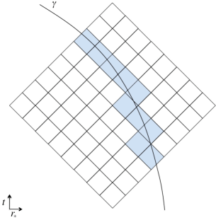
Figure 1: Numerical domain: a staggered 1+1-dimensional mesh in $t$,$r^{*}$ coordinates. The geodesic trajectory of the particle is represented by the continued line $\gamma$. The shadowed cells are those crossed by the particle.

IV.1 The numerical scheme

The jump conditions determined in the previous section are functions of the $t,r$ variables, but for convenience in the following computations, they are transformed into functions of $t,r^{*}$. The integration method considers cells belonging to two groups: for cells which are never crossed by the particle, the integrating approach is drawn by the LPMP method, whereas for cells which are crossed, we propose our strategy.

There are four sub-cases representing the different particle trajectories inside the cell, see Figs. (2 - 5). We define $\alpha,\beta,\gamma,\delta$ the four vertices of the diamond centred on $\sigma$ and initially consider the world line crossing the cell as displayed in Fig. (2). The trajectory crosses the line $\beta$-$\delta$ at the point $a$ and the line $\alpha$-$\gamma$ at the point $b$. We also define the shift $\epsilon_{a}$ and the lapse $\epsilon_{b}$ as $\epsilon_{a}=\text{min}\left\{r^{*}_{a}-r^{*}_{\beta},r^{*}_{\delta}-r^{*}_{a}\right\}$, $\epsilon_{b}=\text{min}\left\{t_{\alpha}-t_{b},t_{b}-t_{\gamma}\right\}$, respectively. The jump conditions at the $a,b$ coordinates express six analytical equations:

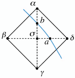
Figure 2: Cell crossed by the particle. The particle crosses the segment $\left[\sigma\delta\right]$ at the point $a$ and the segment $\left[\sigma\alpha\right]$ at the point $b$.

$$\left(\Psi^{+}-\Psi^{-}\right)_{a}=[\Psi]_{a}~{}~{},$$ (34)

$$\left(\Psi^{+}-\Psi^{-}\right)_{b}=[\Psi]_{b}~{}~{},$$ (35)

$$\left(\Psi_{,r^{*}}^{+}-\Psi_{,r^{*}}^{-}\right)_{a}=[\Psi_{,r^{*}}]_{a}~{}~{},$$ (36)

$$\left(\Psi_{,r^{*}}^{+}-\Psi_{,r^{*}}^{-}\right)_{b}=[\Psi_{,r^{*}}]_{b}~{}~{},$$ (37)

$$\left(\Psi_{,t}^{+}-\Psi_{,t}^{-}\right)_{a}=[\Psi_{,t}]_{a}~{}~{},$$ (38)

$$\left(\Psi_{,t}^{+}-\Psi_{,t}^{-}\right)_{b}=[\Psi_{,t}]_{b}~{}~{}.$$ (39)

We maintain the superscript notation for which the wave function values between the world line and infinity are noted by the plus sign, and conversely by the minus sign for the values between the world line and the horizon (incidentally, such notation would also be applicable to the LPMP method).

Using a first order expansion, we get a set of six numerical equations. For case 1, see Fig. (2), they are:

$$\Psi^{+}_{\alpha}=\Psi^{+}(t_{b}+\epsilon_{b},r^{*}_{b})=\Psi^{+}_{b}+\epsilon_{b}\left.\Psi^{+}_{,t}\right|_{b}~{}~{},$$ (40)

$$\Psi^{-}_{\sigma}=\Psi^{-}(t_{b}-(h-\epsilon_{b}),r^{*}_{b})=\Psi^{-}_{b}-(h-\epsilon_{b})\left.\Psi^{-}_{,t}\right|_{b}~{}~{},$$ (41)

$$\Psi^{-}_{\gamma}=\Psi^{-}(t_{b}-2h+\epsilon_{b},r^{*}_{b})=\Psi^{-}(t_{\sigma}-h,r^{*}_{b})=\Psi^{-}_{\sigma}-h\left.\Psi^{-}_{,t}\right|_{\sigma}~{}~{},$$ (42)

$$\Psi^{+}_{\delta}=\Psi^{+}(t_{a},r^{*}_{a}+\epsilon_{a})=\Psi_{a}^{+}+\epsilon_{a}\left.\Psi^{+}_{,r^{*}}\right|_{a}~{}~{},$$ (43)

$$\Psi^{-}_{\sigma}=\Psi^{-}(t_{a},r^{*}_{a}-(h-\epsilon_{a}))=\Psi^{-}_{a}-(h-\epsilon_{a})\left.\Psi^{-}_{,r^{*}}\right|_{a}~{}~{},$$ (44)

$$\Psi^{-}_{\beta}=\Psi^{-}(t_{a},r^{*}_{a}-2h+\epsilon_{a})=\Psi^{-}(t_{\sigma},r^{*}_{\sigma}-h)=\Psi^{-}_{\sigma}-h\left.\Psi^{-}_{,r^{*}}\right|_{\sigma}~{}~{}.$$ (45)

Our aim is the determination of the value of $\Psi^{+}_{\alpha}$, knowing those of $\Psi^{-}_{\beta}$, $\Psi^{-}_{\gamma}$, $\Psi^{+}_{\delta}$, $\epsilon_{a}$, $\epsilon_{b}$, $\left[\Psi\right]_{a,b}$, $\left[\Psi_{,r}\right]_{a,b}$ and $\left[\Psi_{,t}\right]_{a,b}$ To this end, we subtract Eq. (41) from Eq. (40), Eq. (44) from Eq. (43) and obtain, respectively:

$$\Psi^{+}_{\alpha}=\Psi^{-}_{\sigma}+[\Psi]_{b}+\epsilon_{b}[\Psi_{,t}]_{b}+h\left.\Psi^{-}_{,t}\right|_{b}~{}~{},$$ (46)

$$\Psi^{+}_{\delta}=\Psi^{-}_{\sigma}+[\Psi]_{a}+\epsilon_{a}[\Psi_{,r^{*}}]_{a}+h\left.\Psi^{-}_{,r^{*}}\right|_{a}~{}~{}.$$ (47)

Summing Eq. (42) and Eq. (46), Eq. (45) and Eq. (47), and combining the results, we finally get:

$$\Psi^{+}_{\alpha}=\Psi^{-}_{\beta}-\Psi^{-}_{\gamma}+\Psi^{+}_{\delta}-\left[\Psi\right]_{a}+\left[\Psi\right]_{b}-\epsilon_{a}\left[\Psi_{,r^{*}}\right]_{a}+\epsilon_{b}\left[\Psi_{,t}\right]_{b}~{}~{}.$$ (48)

We thus have obtained, without direct integration of the singular source, the value of the upper node. Furthermore, the latter depends solely on analytic expressions, and obviously on the other values at the cell corners. Similar relations are found for the other three cases. For case 2 (Fig. 3), we obtain:

$$\Psi^{+}_{\alpha}=\Psi^{-}_{\beta}-\Psi^{-}_{\gamma}+\Psi^{+}_{\delta}+\left[\Psi\right]_{a}-\left[\Psi\right]_{b}-\epsilon_{a}\left[\Psi_{,r^{*}}\right]_{a}+\epsilon_{b}\left[\Psi_{,t}\right]_{b}~{}~{};$$ (49)

for case 3 (Fig. 4):

$$\Psi^{-}_{\alpha}=\Psi^{-}_{\beta}-\Psi^{-}_{\gamma}+\Psi^{+}_{\delta}-\left[\Psi\right]_{a}-\epsilon_{a}\left[\Psi_{,r^{*}}\right]_{a}~{}~{};$$ (50)

for case 4 (Fig. 5):

$$\Psi^{+}_{\alpha}=\Psi^{-}_{\beta}-\Psi^{+}_{\gamma}+\Psi^{+}_{\delta}+\left[\Psi\right]_{a}-\epsilon_{a}\left[\Psi_{,r^{*}}\right]_{a}~{}~{}.$$ (51)

In a concise form, the four cases might be represented by a single expression (where $\Psi_{\alpha}$ stands for $\Psi^{+}_{\alpha}$ or $\Psi^{-}_{\alpha}$, and $\Psi_{\gamma}$ stands for $\Psi^{+}_{\gamma}$ or $\Psi^{-}_{\gamma}$):

$$\Psi_{\alpha}=\Psi^{-}_{\beta}-\Psi_{\gamma}+\Psi^{+}_{\delta}\mp\left\{\left[\Psi\right]_{a}-B\left[\Psi\right]_{b}\right\}-\epsilon_{a}\left[\Psi_{,r^{*}}\right]_{a}+B\epsilon_{b}\left[\Psi_{,t}\right]_{b}~{}~{},$$ (52)

where the upper sign holds when $r^{*}_{a}>r^{*}_{\sigma}$ and the lower when $r^{*}_{a}<r^{*}_{\sigma}$, $B=0$ if the particle does not cross the $\alpha$-$\gamma$ line, and $B=1$ otherwise.

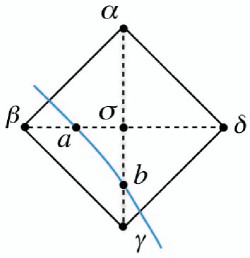
Figure 3: Cell crossed by the particle. The particle crosses the segment $\left[\sigma\gamma\right]$ at the point $b$ and the segment $\left[\sigma\beta\right]$ at the point $a$.

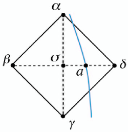
Figure 4: Cell crossed by the particle. The particle crosses the segment $\left[\sigma\delta\right]$ at the point $a$.

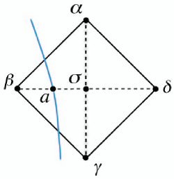
Figure 5: Cell crossed by the particle. The particle crosses the segment $\left[\sigma\beta\right]$ at the point $a$.

V Radiated wave forms at infinity and the wave function at the particle

We confirm the existing wave forms previously published by Lousto and Price lopr97b , and Martel and Poisson mapo02 . In this section, the results from a code based on the LPMP method (full second order) are compared to those obtained by the -I- method (first order for the filled cells, as presented herein, and LPMP-like for empty cells). In spite of the partially different order of the two codes, the difference between the wave forms computed by the two methods is marginal. Incidentally, this occurs in absence of a recognised standard to which refer different numerical approaches.

Figs. 6, 7 show the $l=2$ wave forms for the LPMP and -I- methods, for a particle falling radially, with zero initial velocity, from $r_{u0}/2M=5$ and $r_{u0}/2M=20$, respectively, in units $u=t-r^{*}$, $(2M/m)\Psi$. The initial data are given by the minimal ($\alpha=1$) initial data condition $H_{2}=\alpha K$ for both cases (the parameter $\alpha$, introduced in mapo02 , measures the amount of radiation present on the initial hypersurface and for $\alpha=1$, the initial metric is conformally flat).

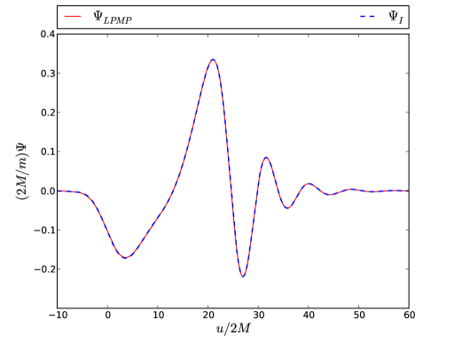
Figure 6: Radiated $l=2$ wave form for a particle falling radially from $r_{u0}/2M=5$ with zero initial velocity, in units $u=t-r^{*}$, $(2M/m)\Psi$. The dashed and solid line represent the -I- and LPMP methods, respectively.

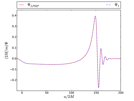
Figure 7: Radiated $l=2$ wave form for a particle falling radially from $r_{u0}/2M=20$ with zero initial velocity, in units $u=t-r^{*}$, $(2M/m)\Psi$. The dashed and solid line represent the -I- and LPMP methods, respectively.

Figs. 8, 9 show the logarithmic (absolute) difference for the $l=2$ wave forms between the LPMP and -I- methods, for a particle falling radially, with zero initial velocity, from $r_{u0}/2M=5$ and $r_{u0}/2M=20$, respectively. It is evinced that the normalised wave function amplitudes differ of an amount between $10^{-3}$ and $10^{-8.5}$, in normalised units.

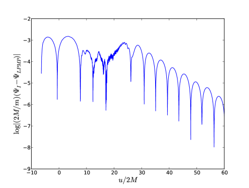
Figure 8: Logarithmic (absolute) difference plot for a particle falling radially from $r_{u0}/2M=5$ with zero initial velocity, in units $u=t-r^{*}$, $(2M/m)\Psi$, between the -I- and LPMP methods ($l=2$).

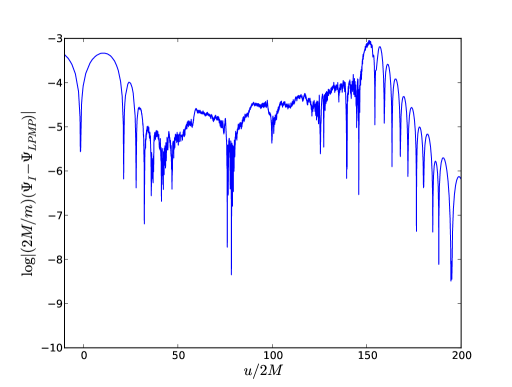
Figure 9: Logarithmic (absolute) difference plot for a particle falling radially from $r_{u0}/2M=20$ with zero initial velocity, in units $u=t-r^{*}$, $(2M/m)\Psi$, between the -I- and LPMP methods ($l=2$).

We show also the behaviour of the wave function at the position of the particle, Figs. (10, 11). The theoretical jump condition, Eq. (29), and the numerical result well overlap at the particle position, as it may be inferred from the logarithmic (absolute) difference plots, Figs. (12,13). The discrepancy in normalised units is between $10^{-3}$ and $10^{-6.5}$.

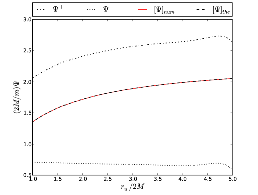
Figure 10: Wave function ($\Psi^{+}$, dashed-dotted line, and $\Psi^{-}$, dotted line) at the particle position for a particle falling radially from $r_{u0}/2M=5$ with zero initial velocity ($l=2$), in units $u=t-r^{*}$, $(2M/m)\Psi$. The numerical jump condition $[\Psi]_{num}$, solid line, and the theoretical jump condition $[\Psi]_{the}$, dashed line Eq. (29), are shown.

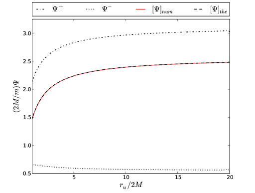
Figure 11: Wave function ($\Psi^{+}$, dashed-dotted line, and $\Psi^{-}$, dotted line) at the particle position for a particle falling radially from $r_{u0}/2M=20$ with zero initial velocity ($l=2$), in units $u=t-r^{*}$, $(2M/m)\Psi$. The numerical jump condition $[\Psi]_{num}$, solid line, and the theoretical jump condition $[\Psi]_{the}$, dashed line Eq. (29), are shown.

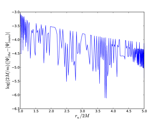
Figure 12: Logarithmic (absolute) difference plot for a particle falling radially from $r_{u0}/2M=5$ with zero initial velocity, in units $u=t-r^{*}$, $(2M/m)\Psi$, at the particle position, between theoretical and numerical jump conditions ($l=2$).

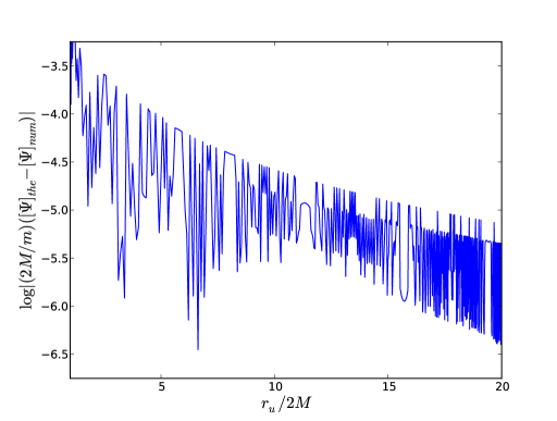
Figure 13: Logarithmic (absolute) difference plot for a particle falling radially from $r_{u0}/2M=20$ with zero initial velocity, in units $u=t-r^{*}$, $(2M/m)\Psi$, at the particle position, between theoretical and numerical jump conditions ($l=2$).

V.1 Discussion

The features of the -I- method can be summarised as follows:

• For the grid cells crossed by the particle, direct and explicit integration of the wave equation, the source term with the associated singularities and the potential, is avoided. This determines also a faster code.

• Reliability is improved, since analytic expressions totally replace the numerical expressions representing the source. The terminology “source-free” is due to this feature.

• A higher order scheme can be written, starting from a higher order Taylor expansion for Eqs. (40-45), and associated to this method rispaoco11 .

• The applicability of the method stretches out to generic orbits. It is our concern to apply the -I- method to circular and eccentric orbits, even if these orbits are not accompanied by perturbations of $C^{0}$ class. The rationale poses on the following consideration. Instead of using the continuity of the perturbations to get the jump conditions, we assume that the even and odd wave equations are satisfied by $\Psi$, respectively $R$, being $C^{-1}$. Using this approach, we have obtained encouraging results for an eccentric orbit aosp11 .

• The disadvantage of this method is represented by the four possible trajectories that a particle may follow inside a given cell, instead of the three possible paths of the LPMP method. A different labeling of the intersections between the particle world line and the cell, though, reduces the number of cases to three rispaoco11 .

VI Conclusions and outlook

We have presented a novel integration method in the time domain for the Zerili-Moncrief wave equation at first order, for cells crossed by the particle world line. The forward time value in the upper node of the $(t,r^{*}$) grid cell is obtained by the linear combination of the three preceding node values and of the analytic jump conditions. Therefore, the numerical integration does not deal any longer with the source term, the associated singularities and the potential. The direct integration of the wave equation is circumvented.

The wave forms at infinity confirm published results, and the wave function at the particle position shows a well-behaved pattern. Our final aim is the evaluation and the application of the back-action at the position of the particle, in a self-consistent manner.

The indirect or source-free method has been developed to fourth order rispaoco11 and applied to generic orbits aosp11 .

Beyond the scenario of EMRIs, other lines of investigation may emerge. One concerns the formal relation between the algorithms of the indirect and LPMP approaches lopr97b ; mapo02 . Another considers applicability of the indirect method to all wave equations with a singular source term, and which the wave function of is constrained by a set of properties.

References

- (1) LISA websites. http://lisa.jpl.nasa.gov http://www.esa.int/science/lisa
- (2) B.S. Sathyaprakash and B.F. Schutz, Classical Quantum Gravity 20, S209 (2003).
- (3) E.K. Porter, arXiv:0910.0373v1 [gr-qc] (2009).
- (4) J.R. Gair and G. Jones, Classical Quantum Gravity 27, 1145 (2007).
- (5) J.R. Gair, I. Mandel, and L. Wen, J. Phys. Conf. Ser. 122, 012037 (2008).
- (6) J.R. Gair, I. Mandel, and L. Wen, Classical Quantum Gravity 25, 184031 (2008).
- (7) N.J. Cornish, arXiv:0804.3323v3 [gr-qc] (2010).
- (8) S. Babak, J.R. Gair, and E.K. Porter, Classical Quantum Gravity 26, 135004 (2009).
- (9) L. Barack and C. Cutler, Phys. Rev. D 70, 122002 (2004).
- (10) E. Racine and C. Cutler, Phys. Rev. D 76, 124033 (2007).
- (11) N.J. Cornish and L.J. Rubbo, Phys. Rev. D 67, 022001 (2003); Publisher’s note, ibidem, 029905 (2003).
- (12) M. Vallisneri, Phys. Rev. D 71,022001 (2005).
- (13) A. Petiteau, G. Auger, H. Halloin, O. Jeannin, E. Plagnol, S. Pireaux, T. Regimbau, and J.-Y. Vinet, Phys. Rev. D 77, 023002 (2008).
- (14) L. Blanchet, A. Spallicci, and B. Whiting Eds., Mass and motion in general relativity, (Springer, Berlin, 2011).
- (15) T. Regge and J.A. Wheeler, Phys. Rev. 108, 1063 (1957).
- (16) A. Nagar, T. Damour, and A. Tartaglia, Classical Quantum Gravity 24, S109 (2007).
- (17) T. Damour and A. Nagar, Phys. Rev. D 76, 064028 (2007).
- (18) S. Bernuzzi and A. Nagar, Phys. Rev. D 81, 084056 (2010).
- (19) T. Damour, Phys. Rev. D 81, 024017 (2010).
- (20) N. Yunes, A. Buonanno, S.A. Hughes, M.C. Miller, and Y. Pan, 2010. Phys. Rev. Lett. 104, 091102 (2010).
- (21) L. Blanchet, S. Detweiler, A. Le Tiec, and B.F. Whiting, Phys. Rev. D 81, 064004 (2010).
- (22) L. Blanchet, S. Detweiler, A. Le Tiec, and B.F. Whiting, Phys. Rev. D 81, 084033 (2010).
- (23) L. Barack, T. Damour, and N. Sago, Phys. Rev. D 82, 084036 (2010).
- (24) U. Sperhake, talk given at the Conference Theory meets data analysis at comparable and extreme mass ratios, 20-26 June 2010 Waterloo (Canada), Perimeter Institute.
- (25) R. Ruffini and J.A. Wheeler, in Significance of space research for fundamental physics, ESRO colloquium, Interlaken 4 September 1969, ESRO-52, A.F. Moore and V. Hardy Eds., (European Space Research Organisation, Paris, 1971), p. 45.
- (26) R. Ruffini and J.A. Wheeler, in The astrophysical aspects of the weak interactions, Cortona 10-12 June 1970, ANL Quaderno n. 157, G. Bernardini, E.Amaldi, and L. Radicati di Brozolo Eds. (Accademia Nazionale dei Lincei, Roma, 1971), p. 165.
- (27) F.J. Zerilli, The gravitational field of a particle falling in a Schwarzschild geometry analyzed in tensor harmonics, Doctorate dissertation, Director: J.A. Wheeler (Princeton Univ., 1969).
- (28) F.J. Zerilli, Phys. Rev. Lett. 24, 737 (1970).
- (29) F.J. Zerilli, J. Math. Phys. 11, 2203 (1970).
- (30) F.J. Zerilli, Phys. Rev. D 2, 2141 (1970); erratum, in Black holes, Les Houches 30 July 31 August 1972, C. DeWitt, B. DeWitt Eds. (Gordon and Breach Science Publ., New York, 1973).
- (31) J. Droste, Kon. Ak. Wetensch. Amsterdam 23, 968 (1915). English translation: Proc. Acad. Sci. Amsterdam 17, 998 (1915).
- (32) J. Droste, Het zwaartekrachtsveld van een of meer lichamen volgens de theorie van Einstein, Doctorate thesis, Dir. H.A. Lorentz (Rijksuniversiteit van Leiden, 1916).
- (33) J. Droste, Kon. Ak. Wetensch. Amsterdam 25, 163 (1916). English translation: Proc. Acad. Sci. Amsterdam 19, 197 (1917).
- (34) K. Schwarzschild, Sitzungsber. Preuss. Akad. Wiss., Phys. Math. Kl., 189 (1916). English translation with foreword by S. Antoci, A. Loinger, arXiv:physics/9905030v1 [physics.hist-ph] (1999).
- (35) T. Rothman, Gen. Rel. Grav. 34, 1541 (2002).
- (36) M. Davis and R. Ruffini, Lett. Nuovo Cimento 2, 1165 (1972).
- (37) M. Davis, M., R. Ruffini, W.H. Press, and R.H. Price, Phys. Rev. Lett. 27, 1466 (1971).
- (38) M. Davis, R. Ruffini, and J. Tiomno, Phys. Rev. D 5, 2932 (1972).
- (39) R. Ruffini, in Black holes, Les Houches 30 July - 31 August 1972, C. DeWitt and B. DeWitt Eds., 451 (Gordon and Breach Science, New York, 1973).
- (40) R. Ruffini, Phys. Rev. D 7, 972 (1973).
- (41) R. Ruffini, in Physics and astrophysics of neutron stars and black holes, Proc. of Int. School of Phys. E. Fermi Course LXV, Varenna 14-26 July 1975, R. Giacconi and R. Ruffini Eds., (North-Holland, Amsterdam and Soc. It. Fisica, Bologna, 1978), p. 287.
- (42) K.P. Chung, Nuovo Cimento B 14, 293 (1973).
- (43) I.G. Dymnikova, Yad. Fiz. 31, 679 (1980). English translation: Sov. J. Nucl. Phys., 31, 353 (1980).
- (44) Y. Tashiro and H. Ezawa, Prog. Theor. Phys. 66, 1612 (1981).
- (45) T. Nakamura., K. Oohara, and Y. Koijma, Progr. Theor. Phys. Suppl. 90, 110 (1987).
- (46) M. Shibata and T. Nakamura, Progr. Theor. Phys. 87, 1139 (1992).
- (47) E. Mitsou, arXiv:1012.2028v2 [gr-qc] (2010).
- (48) C.O. Lousto and R.H. Price, Phys. Rev. D 55, 2124 (1997).
- (49) C.O. Lousto and R.H. Price, Phys. Rev. D 56, 6439 (1997).
- (50) K. Martel and E. Poisson, Phys. Rev. D 66, 084001 (2002).
- (51) Y. Mino, M. Sasaki, and T. Tanaka, Phys. Rev. D 55, 3457 (1997).
- (52) T.C. Quinn and R.M. Wald, Phys. Rev. D 56, 3381 (1997).
- (53) S. Detweiler and B.F. Whiting, Phys. Rev. D 67, 024025 (2003).
- (54) N. Warburton and L. Barack, Phys. Rev. D 81, 084039 (2010).
- (55) T.S. Keidl, A.G. Shah, J.L. Friedman, D.-H. Kim, and L.R. Price, Phys. Rev. D 82, 124012 (2010).
- (56) R.P. Kerr, Phys. Rev. Lett. 11, 237 (1963).
- (57) S.E. Gralla and R.M. Wald, Classical Quantum Gravity 25, 205009 (2008).
- (58) L. Barack and C.O. Lousto, Phys. Rev. D 72, 104026 (2005).
- (59) L. Lorenz, Philos. Mag. Ser. 4 34, 287 (1867).
- (60) B.J. Hunt, The Maxwellians (Cornell University Press, New York, 1991).
- (61) T. de Donder, La gravifique Einsteinienne (Gauthier-Villars, Paris, 1921).
- (62) V. Moncrief, Ann. Phys. (N.Y.) 88, 323 (1974).
- (63) S. Gralla, talk given at the Conference Theory meets data analysis at comparable and extreme mass ratios, 20-26 June 2010 Waterloo (Canada), Perimeter Institute.
- (64) S. Aoudia and A. Spallicci, in preparation.
- (65) P. Ritter, A. Spallicci, S. Aoudia, and S. Cordier, submitted to Classical Quantum Gravity (2011).
- (66) N. Sago, H. Nakano, and M. Sasaki, Phys. Rev. D 67, 104017 (2003).
- (67) H. Nakano. Private communication (2010).
- (68) A. Spallicci, in Mass and motion in general relativity, L. Blanchet, A. Spallicci, and B. Whiting Eds. (Springer, Berlin, 2011).
- (69) C.O. Lousto, Phys. Rev. Lett. 84, 5251 (2000).
- (70) C.O. Lousto and H. Nakano, Classical Quantum Gravity 26, 015007 (2009).
- (71) S. Aoudia and A. Spallicci, in 12th Marcel Grossmann Meeting, Paris 12-18 July 2009, T. Damour, R.T. Jantzen, R. Ruffini Eds. (World Scientific, Singapore, 2011). arXiv:1003.3107v3 [gr-qc] (2010).
- (72) C.F. Sopuerta and P. Laguna, Phys. Rev. D 73, 044028 (2006).
- (73) R. Haas, Phys. Rev. D 75, 124011 (2007).
- (74) S.E. Field, J.S. Hesthaven, and S.R. Lau, Classical Quantum Gravity 26, 165010 (2009)