IPM/P-2010/032

Abstract

We use the AdS/CFT correspondence to study the DC conductivity of massive $\mathcal{N}=2$ hypermultiplet fields in an $\mathcal{N}=4\,SU(N_{c})$ super-Yang-Mills theory plasma in the large $N_{c}$ and finite ’t Hooft coupling. We also discuss general curvature-squared and Gauss-Bonnet corrections on the DC conductivity.

1 Introduction

Anti-de Sitter/conformal field theory correspondence ($AdS/CFT$) conjectures that IIB string theory on $AdS_{5}\times S^{5}$ background is dual to $D=4\ {\cal{N}}=4\ SU(N_{c})$ super Yang-Mills theory (SYM) [1]. In the limits of large $N_{c}$ and large ’t Hooft coupling $\lambda=g_{YM}N_{c}^{2}$, the SYM theory is dual to IIb supergravity which is low energy effective theory of superstring theory. As a result a thermal SYM theory corresponds to supergravity in an AdS-Schwarzschild background where the SYM theory temperature is identified with the Hawking temperature of the $AdS$ black hole [2].

$AdS/CFT$ idea has been applied to study different aspects of strongly coupled SYM theory. Recently the application of this duality in condensed matter physics (called $AdS/CMT$) has been studied [3] . This duality is very useful to study certain strongly coupled systems in $CMT$ by holography techniques and to understand better their properties. A quantity attracting attentions and computing is conductivity [4]. In order to compute conductivity, it is necessary to add spinor fields in fundamental representation. As it is well-known fields in the $\mathcal{N}=4$ SYM theory are in adjoint representation and by introducing $\mathcal{N}=2$ hypermultiplets one can include fields in the fundamental representation. To do so on gravity side, $N_{f}$ flavor branes are introduced in the probe limit meaning we have only $N_{f}\ll N_{c}$ of them and the $AdS$ background is left unchanged. In other words, open string degrees of freedom are now considered. On the gauge theory side this corresponds to ${\cal{N}}=2$ supersymmetric hypermultiplet flavor fields propagating in SYM theory. The local $U(N_{f})$ symmetry on the D7-branes corresponds to global $U(N_{f})$ symmetry whose $U(1)_{B}$ subgroup may be identified with baryon number. Non-dynamical electric and magnetic fields can be coupled to $U(1)_{B}$ charge and we then expect a constant, nonzero currents. Hence the conductivity tensor $\sigma_{ij}$ is identified by

$$<J_{i}>=\sigma_{ij}E_{j}\,.$$ (1)

Electric and magnetic fields produce diagonal and off-diagonal elements in conductivity tensor respectively. In fact on the gravity side currents, electric and magnetic fields are introduced as nontrivial gauge fields living on the D7-branes.

The DC conductivity in ”strange metals” has been studied in [7, 8]. It was found that conductivity is independent of the dimensionality of a probe brane in the background created by a stack of D_p-branes [6]. Also it was shown that the properties of the DC conductivity can be studied by that of the single heavy quark. One should consider massive carriers as endpoint of strings which end on flavor branes and use the quasi-particle description. Then it would be straightforward to calculate the DC conductivity from the drag force calculations[8, 9]. We discuss this approach in the last section.

In this paper we study higher derivative corrections on the DC conductivity. These corrections on the gravity side correspond to finite coupling corrections on the gauge theory side. The main motivation to consider corrections comes from the fact that string theory contains higher derivative corrections arising from stringy effects. In the case of $\mathcal{N}=4$ SYM theory, the leading order correction in $1/\lambda$ arises from stringy correction to the low energy effective action of type $\amalg$b supergravity, $\alpha^{\prime 3}{\cal{R}}^{4}$. We study ${\cal{R}}^{4}$ and ${\cal{R}}^{2}$ corrections to the DC conductivity. An understanding of how these computations are affected by finite $\lambda$ corrections may be essential for more precise theoretical predictions.

The article is organized as follows. In the next section, we will give a brief review of [4, 5] and then follow the same direction and study Ohmic and Hall conductivities in the presence of corrections in section 3. Moreover in section 4, we consider general ${\cal{R}}^{2}$ and Gauss-Bonnet corrections and in the last section we draw our conclusions and summarize our results.

2 Review of conductivity

In this section we will give a brief review of [4, 5]. The AdS-Schwarzchild metric, in units where the radius of $AdS$ is one, is

$$ds^{2}=G_{tt}\ dt^{2}+G_{xx}d\vec{x}^{2}+G_{uu}\ du^{2}+d^{2}\Omega_{5}\,.$$ (2)

Here $d\vec{x}^{2}$ is the three dimensional space and the metric functions are given by

$$G_{tt} =-u^{2}(1-\frac{u_{0}^{4}}{u^{4}}),$$ (3a)

$$G_{xx} =u^{2},$$ (3b)

$$G_{uu} =u^{-2}(1-\frac{u_{0}^{4}}{u^{4}})^{-1},$$ (3c)

where $u_{0}$ is event horizon. Also $S^{5}$ metric is

$$d\Omega_{5}^{2}=d\theta^{2}+sin^{2}\theta\,d\psi^{2}+cos^{2}\theta^{2}\,d\Omega_{3}^{2}\,.$$ (4)

where $d\Omega_{3}^{2}$ is the metric of $S^{3}$ and $\theta$ runs from zero to $\frac{\pi}{2}$. In addition the Hawking temperature is given by

$$T=\frac{u_{0}}{\pi}\,.$$ (5)

In order to find conductivity a number $N_{f}$ of D7-branes filling $AdS_{5}$ and wrapping the $S^{3}\subset S^{5}$ have been considered in the AdS-Schwarzchild background. Moreover worldvolume gauge fields $A_{t}(u)$, $A_{x}(u,t)=-Et+f_{x}(u)$ and $A_{y}(u,t)=Bx+f_{y}(u)$ as well as the $\theta(u)$ describing the position $S^{3}$ on the $S^{5}$ are turned on. The above system is described by Dirac-Born-Infeld action. From the gauge field equations of motion, conserved charges $Q$, $I^{x}$ and $I^{y}$ associated with $A_{t}(u)$, $A_{x}(u,t)$ and $A_{y}(u,t)$ are found. The conserved charges which are sub-leading, normalizable terms of asymptotic expansion can be related to expectation value of dual operators i.e.

$$<J^{t}>=Q,\ \ \ \ <J^{x}>=I^{x},\ \ \ \ <J^{y}>=I^{y}.$$ (6)

Having worked out the gauge fields in terms of $Q$ and $B$ one can write the on-shell action as follows [5]

$$S_{D7}=-{\cal{N}}^{2}(2\pi\alpha^{\prime})^{2}\int\,d^{4}xcos^{6}\theta\,g_{xx}^{2}\,\sqrt{g_{tt}g_{uu}}\frac{\xi}{\sqrt{\xi\chi-a^{2}}},$$ (7)

where ${\cal{N}}=\frac{\lambda}{(2\pi^{4})}N_{f}N_{c}$. $g_{tt}(=|g_{tt}|),\ g_{uu}$ and $g_{xx}$ are components of induced metric and

$$\xi =g_{tt}g_{xx}^{2}+(2\pi\alpha^{\prime})^{2}(g_{tt}B^{2}-g_{xx}E^{2}),$$ (8a)

$$\chi =g_{tt}g_{xx}^{2}\left({\cal{N}}^{2}(2\pi\alpha^{\prime})^{4}g_{xx}\cos^{6}\theta\right)+(2\pi\alpha^{\prime})^{2}\left(g_{tt}Q^{2}-g_{xx}(I_{x}^{2}+I_{y}^{2})\right),$$ (8b)

$$a =(2\pi\alpha^{\prime})^{2}\left(g_{tt}I^{x}B+g_{xx}I^{y}E\right).$$ (8c)

$\xi$, as a function of $u$, has negative and positive value at the horizon and near the boundary respectively. In fact at a specific point, say $u_{*}$, we have $\xi(u_{*})=0$. Hence $u_{*}$ is

$$u_{*}^{4}=u_{0}^{4}{\cal{F}}(e,b)=\pi^{4}T^{4}{\cal{F}}(e,b)=g_{xx}^{2}(u_{*})$$ (9)

where

$$\begin{split}{\cal{F}}(e,b)&=\frac{1}{2}\left(1+e^{2}-b^{2}+\sqrt{(1+e^{2}-b^{2})^{2}+4b^{2}}\right)\cr e&=\frac{E}{\frac{\pi}{2}\sqrt{\lambda}T^{2}},\ \ b=\frac{B}{\frac{\pi}{2}\sqrt{\lambda}T^{2}},\ \ q=\frac{Q}{\frac{\pi}{2}\sqrt{\lambda}T^{2}}\end{split}$$ (10)

Reality condition of $\sqrt{\xi\chi-a^{2}}$ imposes that two functions $\chi$ and $a$ must vanish at $u=u_{*}$. By setting (8b) and (8c) to zero at $u_{*}$ and converting to field theory quantities, Ohmic and Hall conductivities become

$$\sigma_{xx} =\sqrt{\frac{N_{f}^{2}N_{c}^{2}\cos^{6}\theta_{*}}{16\pi^{2}}\frac{{\cal{F}}^{3/2}}{b^{2}+{\cal{F}}}T^{2}+\frac{q^{2}{\cal{F}}}{(b^{2}+{\cal{F}})^{2}}}$$ (11a)

$$\sigma_{xy} =\frac{qb}{b^{2}+{\cal{F}}}$$ (11b)

The Ohmic conductivity depends on magnetic field, electric field and the temperature of the field theory, simplicity we name it as $\sigma(B,E,T)$. This quantity has two main terms

$$\sigma_{xx}(B,E,T)=\sqrt{\hat{\sigma}_{0}^{2}+\hat{\sigma}^{2}}$$ (12)

where $\hat{\sigma}_{0}$ arises from thermally produced pairs of charge carriers. By increasing the mass of carriers, $\hat{\sigma}_{0}$ can be made arbitrary small and the leading term in conductivity will be $\hat{\sigma}$. This term can be found by studying the properties of a moving single string and calculating drag force [4]. We will discuss this point in the discussion section.

In next section we will follow the same direction and study above conductivities in the presence of correction.

3 ${\cal{R}}^{4}$ corrections to AdS-Schwarzschild black brane

Since $AdS/CFT$ correspondence refers to complete string theory, one should consider the string corrections to the 10D supergravity action. The first correction occurs at order $(\alpha^{\prime})^{3}$ [13]. In the extremal $AdS_{5}\times S^{5}$ it is clear that the metric does not change [14], conversely this is no longer true in the non-extremal case. Corrections in inverse ’t Hooft coupling $1/\lambda$ which correspond to $\alpha^{\prime}$ corrections on the string theory side were found in [13]. Higher derivative corrections i.e. ${\cal{R}}^{2}$ and ${\cal{R}}^{4}$ on the rotating quark-antiquark system in the hot plasma and on the drag force on a moving heavy quark have been investigated in [10, 11, 12].

Functions of the $\alpha^{\prime}$-corrected metric are given by [15]

$$G_{tt} = -u^{2}(1-w^{-4})T(w),$$

$$G_{xx} = u^{2}X(w),$$

$$G_{uu} = u^{-2}(1-w^{-4})^{-1}U(w),$$ (13)

where

$$T(w) = 1-k\bigg{(}75w^{-4}+\frac{1225}{16}w^{-8}-\frac{695}{16}w^{-12}\bigg{)}+\dots,$$

$$X(w) = 1-\frac{25k}{16}w^{-8}(1+w^{-4})+\dots,$$

$$U(w) = 1+k\bigg{(}75w^{-4}+\frac{1175}{16}w^{-8}-\frac{4585}{16}w^{-12}\bigg{)}+\dots,\$$ (14)

and $w=\frac{u}{u_{0}}$. There is an event horizon at $u=u_{0}$ and the geometry is asymptotically $AdS$ at large $u$ with a radius of curvature $R=1$. The expansion parameter $k$ can be expressed in terms of the inverse ’t Hooft coupling as

$$k=\frac{\zeta(3)}{8}\lambda^{-3/2}\sim 0.15\lambda^{-3/2}.$$ (15)

The temperature is given by

$$T_{{\cal{R}}^{4}}=\frac{u_{0}}{\pi(1-k)}.$$ (16)

In order to find conductivities we set all of equations (8) to zero where the induced metric components will now be computed by (3).

3.1 Ohmic conductivity

Here we focus on a case where the magnetic field has been turned off and (8a), after setting to zero, becomes

$$\begin{split}w^{16}-(1+75k+e^{2})w^{12}-k\left(\frac{25}{8}w^{8}-120\,w^{4}+\frac{335}{8}\right)=0,\end{split}$$ (17)

up to first order in $k$ perturbatively. $u_{*}=u_{0}w_{*}$ is a real parameter and takes value between $u_{0}$ and infinity. These two conditions tell us that just a root of (17) is acceptable for $w_{*}$ among sixteen roots. Now (8b) and (8c) must be set to zero. (8c) leads to $I^{y}=0$ and (8b) becomes

$$\sigma_{xx}=\frac{I^{x}}{E}=\sqrt{{\cal{N}}^{2}(2\pi\alpha^{\prime})^{4}g_{xx}\cos^{6}\theta_{*}+\frac{(2\pi\alpha^{\prime})^{2}}{g_{xx}^{2}}Q^{2}}\,.$$ (18)

where $g_{xx}$ evaluated at $u_{*}$, which is found by solving (17), is given by

$$g_{xx}(u_{*})=\pi^{2}T^{2}\left(\sqrt{1+e^{2}}+\frac{5k\left(-10+e^{2}\left(163+120e^{2}\left(3+e^{2}\right)\right)\right)}{16\left(1+e^{2}\right)^{7/2}}\right),$$ (19)

Finally by substituting (19) in (18) the Ohmic conductivity becomes

$$\begin{split}\sigma^{\mathcal{R}^{4}}_{xx}&=\sigma^{\mathcal{N}=4}_{xx}+\cr&\frac{5\,\zeta(3)\,\lambda^{-3/2}}{256\,\left(1+e^{2}\right)^{4}}\,\bigg{(}-10+e^{2}\left(163+120e^{2}\left(3+e^{2}\right)\right)\bigg{)}\,\bigg{(}\sigma^{\mathcal{N}=4}_{xx}-\frac{3\frac{q^{2}}{1+e^{2}}}{\sigma^{\mathcal{N}=4}_{xx}}\bigg{)}\,,\end{split}$$ (20)

where

$$\sigma^{{\mathcal{N}=4}}_{xx}=\sqrt{\frac{N_{f}^{2}N_{c}^{2}T^{2}}{16\pi^{2}}\sqrt{1+e^{2}}\cos^{6}\theta_{*}+\frac{q^{2}}{1+e^{2}}}\,.$$ (21)

We would like to emphasize two points about our result. First, at finite temperature for a large value of electric field second term in the conductivity equation coming from correction goes to zero which means that correction of metric is negligible. Second, depending on other parameters, conductivity increases, decreases or does not change. In particular by taking large mass limit $\cos\theta_{*}\rightarrow 0$ [1, 2] there is a critical value of electric field $e_{c}=0.233745$ where the correction effect vanishes. As a result conductivity increases when $e<e_{c}$ and vice versa. In the limit of zero density, if $e>e_{c}$ or $e<e_{c}$ we have a positive or negative correction effect, respectively.

3.2 Conductivities in the presence of magnetic field

In this section, we study the effect of ’t Hooft coupling correction on the conductivities when the magnetic field is turned on. In order to do that by setting (8) to zero, we have

$$w(w -1)(16w^{3}-1200kw^{2}-1275kw+645k)+e^{2}w(-16w^{3}+25kw+25k)$$ (22a)

$$+b^{2}(w-1)(16w^{3}-1200kw^{2}-1225kw+695k)=0,$$

$$\sigma_{xx} =\frac{g_{xx}}{g_{xx}^{2}+(2\pi\alpha^{\prime})^{2}B^{2}}\sqrt{(2\pi\alpha^{\prime})^{4}{\cal{N}}(g_{xx}^{2}+(2\pi\alpha^{\prime})^{2}B^{2})g_{xx}\cos^{6}\theta_{*}+(2\pi\alpha^{\prime})^{2}Q^{2}},$$ (22b)

$$\sigma_{xy} =\frac{(2\pi\alpha^{\prime})^{2}QB}{g_{xx}^{2}+(2\pi\alpha^{\prime})^{2}B^{2}}\,.$$ (22c)

where as before $g_{xx}$ and $\cos\theta$ in (22b) and (22c) are evaluated at $w=w_{*}$. In this case $w_{*}$ will be found by solving (22a). However this equation is complicated one can solve it numerically. We assume different values for parameters and discuss behavior of Ohmic and Hall conductivities in terms of them. In the massive case, $\cos\theta\rightarrow 0$, we have plotted conductivities versus $e$ and $b$ in Fig. 1-4. Our figures have been plotted at fixed temperature($u_{0}=3$) and for three different values of $k$(=0.0001,0.001,0.01).

Ohmic conductivity has been plotted in Fig. 1. In the left plot of this figure $b=10$. Notice that from (15), increasing $k$ corresponds to decreasing ’t Hooft coupling constant $\lambda$. For small values of $\lambda$, there is a specific maximum value for Ohmic conductivity. It is clearly seen that by increasing ’t Hooft coupling constant the shape of Ohmic conductivity changes and it approximately starts from its maximum value. In the right plot of Fig. 1 $b=30$. As one finds from (22), by increasing $b$ the value of Ohmic conductivity will be decreased. This behavior of Ohmic conductivity is clearly shown in this plot. In addition by increasing $b$, the maximum value of Ohmic conductivity appears at larger value of $e$.

,

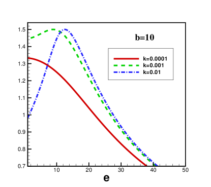
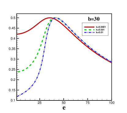
Figure 1: $\sigma_{xx}$ versus $e$ for different values of $k$ at fixed $b$. Left: $b=10$. Right: $b=30$.

It would also be interesting to investigate behavior of Ohmic conductivity in terms of $b$ at constant $e$. In the left and right plots of Fig 2, we have plotted Ohmic conductivity for $e=10$ and $e=20$, respectively. As it is clear from these plots Ohmic conductivity starts from a maximum value and by increasing $b$ it decreases. The main effect of increasing ’t Hooft coupling constant is to decrease Ohmic conductivity value. The right plot of Fig 2 shows the same results. The point is that increasing the value of $e$ causes a decreasing of Ohmic conductivity value.

,

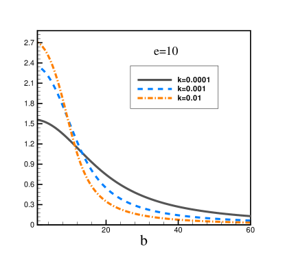
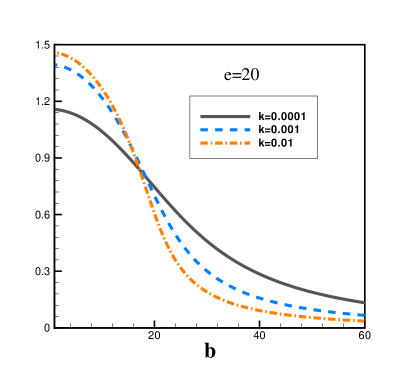
Figure 2: $\sigma_{xx}$ versus $b$ for different values of $k$ at fixed $e$. Left: $e=10$. Right: $e=20$.

In following two paragraphs we study Hall conductivity versus $e$ and $b$. Hall conductivity in terms of $e$ is plotted in Fig. 3 at constant $b$. In the left plot of this figure $b=10$. It is clearly seen that Hall conductivity also starts from its maximum value and it decreases by increasing $e$. Moreover if ’t Hooft coupling constant increases, the maximum value of Hall conductivity will decrease. Comparing with the left plot of Fig. 3, in the right plot Hall conductivity has a smaller value. This fact, which Hall conductivity decreases by increasing $b$, is consistent with (22c).

,

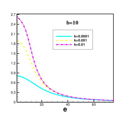
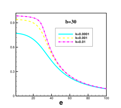
Figure 3: $\sigma_{xy}$ versus $e$ for different values of $k$ at fixed $b$. Left: $b=10$. Right: $b=30$.

,

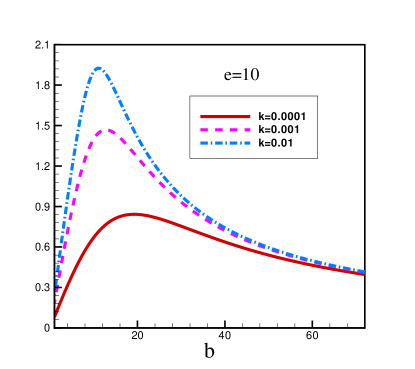
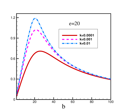
Figure 4: $\sigma_{xy}$ versus $b$ for different values of $k$ at fixed $e$. Left: $e=10$. Right: $e=20$.

Hall conductivity versus $b$ is plotted in Fig. 4 at constant $e$. Two cases, which are $e=10$ and $e=20$, are considered. As it is obviously seen, similar to Fig. 2 and 3, there is a maximum value for Hall conductivity. By increasing ’t Hooft coupling constant this maximum value decreases and in fact this is the most important effect of ’t Hooft coupling correction on the Hall conductivity. The right plot of Fig. 4 indicates that Hall conductivity has a smaller value when $e=20$.

4 ${\cal{R}}^{2}$ corrections to AdS-Schwarzschild black brane

We consider the curvature-squared corrections on the AdS black brane solution and study DC conductivity in this background. ${\cal{R}}^{2}$ corrections have been introduced in [16, 17]. It is important to point out that the first higher derivative correction in weakly curved type IIb backgrounds enters at order $\mathcal{R}^{4}$, and not $\mathcal{R}^{2}$, so we will not predict effect of curvature-squared corrections on the $\mathcal{N}=4$ SU(N) SYM. At first we consider the general $\mathcal{R}^{2}$ corrections in (23) and calculate Ohmic conductivity and then extend the calculation to the case of Gauss-Bonnet (GB) gravity. Fortunately, we find analytic results in both cases. Hall conductivity in the presence of curvature-squared corrections can be studied, too. Here we only discuss Ohmic conductivity.

The black brane solution of $AdS_{5}$ space with the curvature-squared corrections is [18]

$$ds^{2}=-\kappa(\frac{u^{2}}{R^{2}})f(u)dt^{2}+(\frac{u^{2}}{R^{2}})d\vec{x}^{2}+\frac{1}{(\frac{u^{2}}{R^{2}})f(u)}du^{2},$$ (23)

where

$$f(u)=1-\frac{u_{0}^{4}}{u^{4}}+\alpha+\gamma\frac{u_{0}^{8}}{u^{8}}.$$ (24)

and $\alpha$ and $\gamma$ are small variables. The scaling factor $\kappa=\frac{1}{1+\alpha}$ was included for the speed of light in the boundary to be unity. Also $u$ denotes the radial coordinate of the black brane geometry and $t,\vec{x}$ label the directions along the boundary at the spatial infinity. In these coordinates the event horizon is located at $f(u_{0})=0$ where $u_{0}$ can be found by solving this equation. The boundary is located at infinity and the geometry will be asymptotically AdS with a radius of curvature $R=1$. The temperature is given by

$$T_{\mathcal{R}^{2}}=\frac{u_{0}}{\pi}\left(1+\frac{1}{4}\alpha-\frac{5}{4}\gamma\right).$$ (25)

As what it was done in section 3.1, (8a) after setting to zero, becomes

$$w\left((1+\alpha)w+\frac{e^{2}}{\kappa}(1+\frac{\alpha}{4}-\frac{5\gamma}{4})^{4}-1\right)+\gamma=0,$$ (26)

where

$$e=\frac{E}{\frac{\pi}{2}\sqrt{\lambda}\,T_{\mathcal{R}^{2}}^{2}}.$$ (27)

Obviously by setting $\alpha$ and $\gamma$ to zero one must find Ohmic conductivity in AdS-Schwarzschild background brought in (21). This virtue selects an acceptable root of (26) which was already called $w_{*}$. It is then straightforward to find Ohmic conductivity from (18) that is given by

$$\begin{split}(\sigma^{\mathcal{R}^{2}}_{xx})^{2}&=\frac{512\,(1+\alpha)q^{2}}{256+(1+\alpha)\left(4+\alpha-5\gamma\right)^{4}\,e^{2}+\sqrt{M\left(\alpha,\gamma,e\right)}}\cr&+\frac{1}{(16\pi)^{2}\sqrt{2}}\frac{N_{c}^{2}N_{f}^{2}T^{2}_{\mathcal{R}^{2}}}{(1+\frac{\alpha}{4}-\frac{5}{4}\gamma)^{2}}\cos^{6}{\theta_{*}}\cr&\times\left(\frac{256+(1+\alpha)\left(4+\alpha-5\gamma\right)^{4}\,e^{2}+\sqrt{M\left(\alpha,\gamma,e\right)}}{1+\alpha}\right)^{\frac{1}{2}},\end{split}$$ (28)

where

$$M\left(\alpha,\gamma,e\right)=-2^{18}\,\gamma(1+\alpha)+\left(256+(1+\alpha)(4+\alpha-5\gamma)^{4}\,e^{2}\right)^{2},$$ (29)

and

$$q=\frac{Q}{\frac{\pi}{2}\sqrt{\lambda}\,T_{\mathcal{R}^{2}}^{2}}.$$ (30)

Regarding to small values of $\alpha$ and $\gamma$, as it is expected, the above Ohmic conductivity reproduces (21) for large value of electric field at fixed temperature. Moreover, as original case introduced in [4], although two types of charge carries contribute to the conductivity, which are charge carries represented by $q$ and charge carries thermally produced, the value of them are corrected by ${\mathcal{R}^{2}}$ correction. For example as it was pointed out in (12), in the case of massive charge carriers $\hat{\sigma}$ dominates in (28). Based on the small values of $\alpha$ and $\gamma$, we expand this term and keep only first order terms as

$$(\hat{\sigma}_{\mathcal{R}^{2}})^{2}=(\hat{\sigma})^{2}\left(1+\left(\frac{1-e^{2}}{1+e^{2}}\right)\alpha+\frac{1+5e^{2}+5e^{4}}{(1+e^{2})^{2}}\gamma\right),$$ (31)

where

$$(\hat{\sigma})^{2}=\frac{q}{1+e^{2}}.$$ (32)

In five dimensions, the most general theory of gravity with quadratic powers of curvature is GB theory. The exact solutions and thermodynamic properties of the black brane in GB gravity were discussed in [19, 20, 21]. We are going to more understand about the DC conductivity in the GB gravity. The black brane solution in this geometry is given by [19]

$$ds^{2}=-a\,\frac{u^{2}}{R^{2}}\,h(u)\,dt^{2}+\frac{du^{2}}{\frac{u^{2}}{R^{2}}h(u)}+\frac{u^{2}}{R^{2}}\,d\vec{x}^{2},$$ (33)

where

$$h(u)=\frac{1}{2\lambda_{GB}}\left[1-\sqrt{1-4\lambda_{GB}\left(1-\frac{u_{0}^{4}}{u^{4}}\right)}\right].$$ (34)

In (33), $a$ is an arbitrary constant which specifies the speed of light of the boundary gauge theory and we choose it to be unity. As a result at the boundary, where $u\rightarrow\infty$,

$$h(u)\rightarrow\frac{1}{a},\,\,\,\,\,a=\frac{1}{2}\left(1+\sqrt{1-4\lambda_{GB}}\right).$$ (35)

We assume $\lambda_{GB}\leq\frac{1}{4}$, the reason is that beyond this point there is no vacuum AdS solution and one cannot have a conformal field theory at the boundary. The temperature is given by

$$T_{GB}=\frac{\sqrt{a}\,\,u_{0}}{\pi\,}.$$ (36)

In this case (8a) and (18) lead to

$$w^{4}\left(1-\sqrt{1-4\lambda_{GB}(1-\frac{1}{w})}\right)-2ae^{2}\lambda_{GB}=0,$$ (37)

and

$$\begin{split}(\sigma^{GB}_{xx})^{2}&=\frac{4\,q^{2}}{2(1+ae^{2})+\sqrt{2g\left(\lambda_{GB},e\right)}}\cr&+\frac{1}{32\pi^{2}\,a}N_{c}^{2}N_{f}^{2}\,T^{2}_{GB}\cos^{6}{\theta_{*}}\left(2(1+ae^{2})+\sqrt{2g\left(\lambda_{GB},e\right)}\right)^{\frac{1}{2}},\end{split}$$ (38)

where

$$g(\lambda_{GB},e)=2(1+2ae^{2})+2e^{4}(a-\lambda_{GB})(1+\lambda_{GB}),$$ (39)

and

$$e=\frac{E}{\frac{\pi}{2}\sqrt{\lambda}\,T_{GB}^{2}},\,\,q=\frac{Q}{\frac{\pi}{2}\sqrt{\lambda}\,T_{GB}^{2}}.$$ (40)

It is clearly seen that by setting $\lambda_{GB}=0$, one finds the Ohmic conductivity in AdS-Schwarzschild background. Interpretation of two terms contributing to Ohmic conductivity in (38) is the same as ${\mathcal{R}^{2}}$ correction case.

5 Discussion and Conclusion

In this paper effect of curvature correction on DC conductivity is studied. In particular we considered ${\cal{R}}^{4}$ correction to AdS-Schwarzschild black brane. Our results show that there is a critical value for electric field in which correction to Ohmic conductivity vanishes. Moreover it was shown that, depending on other parameters, Ohmic conductivity can increase or decrease. In another case, when magnetic field is turned on, Hall and Ohmic conductivities are plotted in Fig. 1-4. At fixed temperature and large magnetic field, Ohmic and Hall conductivity generally start from their maximum value. Fig. 4 shows that Hall conductivity has a maximum value at fixed electric field and temperature.

Curvature-squared and Gauss-Bonnet corrections are then considered in the next section. As it is expected, the main structure of Ohmic conductivity is preserved by corrections.

It is straightforward to calculate the DC conductivity from the drag force calculations. One should consider massive carriers as endpoint of strings which end on flavor branes and using the quasi-particle description write the equation of motion for them at the equilibrium where the external force is $f=E$. At large mass limit, only charge carriers contribute to current and one may express $\langle J^{x}\rangle$ in terms of velocity of the quasi-particles, $\langle J^{x}\rangle=\langle J^{t}\rangle\,v$. Regarding Ohm’s law, we have $v=\frac{\sigma\,E}{\langle J^{t}\rangle}$, where $v$ is velocity of massive carrier and it is constant. One can follow this approach and derive $\hat{\sigma}$ in the case of $\mathcal{R}^{2}$ and Gauss-Bonnet corrections in (28) and (38). This approach has been followed in the case of strange metals in [7, 8].

References

- [1] J. M. Maldacena, “The large N limit of superconformal field theories and supergravity,” Adv. Theor. Math. Phys. 2 (1998) 231 [Int. J. Theor. Phys. 38 (1999) 1113] [arXiv:hep-th/9711200]. S. S. Gubser, I. R. Klebanov and A. M. Polyakov, “Gauge theory correlators from non-critical string theory,” Phys. Lett. B 428 (1998) 105 [arXiv:hep-th/9802109]. E. Witten, “Anti-de Sitter space and holography,” Adv. Theor. Math. Phys. 2 (1998) 253 [arXiv:hep-th/9802150].
- [2] E. Witten, “Anti-de Sitter space, thermal phase transition, and confinement in gauge theories,” Adv. Theor. Math. Phys. 2 (1998) 505 [arXiv:hep-th/9803131].
- [3] S. A. Hartnoll, “Lectures on holographic methods for condensed matter physics,” Class. Quant. Grav. 26, 224002 (2009) [arXiv:0903.3246 [hep-th]]; C. P. Herzog, “Lectures on Holographic Superfluidity and Superconductivity,” J. Phys. A 42, 343001 (2009) [arXiv:0904.1975 [hep-th]]; J. McGreevy, “Holographic duality with a view toward manybody physics,” arXiv:0909.0518 [hep-th]; arXiv:1002.1722 [hep-th]; S. Sachdev, “Condensed matter and AdS/CFT,” arXiv:1002.2947 [hep-th].
- [4] A. Karch and A. O’Bannon, ‘Metallic AdS/CFT,” JHEP 0709 (2007) 024 [arXiv:0705.3870 [hep-th]].
- [5] A. O’Bannon, “Hall Conductivity of Flavor Fields from AdS/CFT,” Phys. Rev. D 76 (2007) 086007 [arXiv:0708.1994 [hep-th]].
- [6] A. Karch, M. Kulaxizi and A. Parnachev, “Notes on Properties of Holographic Matter,” JHEP 0911 (2009) 017 [arXiv:0908.3493 [hep-th]].
- [7] S. A. Hartnoll, J. Polchinski, E. Silverstein and D. Tong, “Towards strange metallic holography,” JHEP 1004 (2010) 120 [arXiv:0912.1061 [hep-th]]. T. Faulkner, N. Iqbal, H. Liu, J. McGreevy and D. Vegh, “From black holes to strange metals,” arXiv:1003.1728 [hep-th]. B. H. Lee and D. W. Pang, “Notes on Properties of Holographic Strange Metals,” arXiv:1006.4915 [hep-th].
- [8] K. B. Fadafan, “Drag force in asymptotically Lifshitz spacetimes,” arXiv:0912.4873 [hep-th].
- [9] C. Charmousis, B. Gouteraux, B. S. Kim, E. Kiritsis and R. Meyer, “Effective Holographic Theories for low-temperature condensed matter systems,” arXiv:1005.4690 [hep-th].
- [10] M. Ali-Akbari and K. Bitaghsir Fadafan, “Rotating mesons in the presence of higher derivative corrections from gauge-string duality,” Nucl. Phys. B 835, 221 (2010) [arXiv:0908.3921 [hep-th]].
- [11] K. B. Fadafan, “Charge effect and finite ’t Hooft coupling correction on drag force and Jet Quenching Parameter,” arXiv:0809.1336 [hep-th].
- [12] K. B. Fadafan, “ curvature-squared corrections on drag force,” JHEP 0812 (2008) 051 [arXiv:0803.2777 [hep-th]]. J. F. Vazquez-Poritz, “Drag force at finite ’t Hooft coupling from AdS/CFT,” [arXiv:0803.2890 [hep-th]];
- [13] J. Pawelczyk and S. Theisen, AdS black hole metric at O(), JHEP 9809 (1998) 010, [hep-th/9808126];
- [14] T. Banks and M. B. Green, “Non-perturbative effects in AdS(5) x S**5 string theory and d = 4 SUSY Yang-Mills,” JHEP 9805, 002 (1998) [arXiv:hep-th/9804170];
- [15] S.S. Gubser, I.R. Klebanov and A.A. Tseytlin, Coupling constant dependence in the thermodynamics of supersymmetric Yang-Mills theory Nucl. Phys. B534 (1998) 202, [hep-th/9805156];
- [16] M. Blau, K. S. Narain and E. Gava, “On subleading contributions to the AdS/CFT trace anomaly,” JHEP 9909 (1999) 018 [arXiv:hep-th/9904179].
- [17] A. Fayyazuddin and M. Spalinski, “Large N superconformal gauge theories and supergravity orientifolds,” Nucl. Phys. B 535 (1998) 219 [arXiv:hep-th/9805096].
- [18] Y. Kats and P. Petrov, “Effect of curvature squared corrections in AdS on the viscosity of the dual gauge theory,” arXiv:0712.0743 [hep-th].
- [19] R. G. Cai, “Gauss-Bonnet black holes in AdS spaces,” Phys. Rev. D 65 (2002) 084014 [arXiv:hep-th/0109133].
- [20] S. Nojiri and S. D. Odintsov, “Anti-de Sitter black hole thermodynamics in higher derivative gravity and new confining-deconfining phases in dual CFT,” Phys. Lett. B 521 (2001) 87 [Erratum-ibid. B 542 (2002) 301] [arXiv:hep-th/0109122].
- [21] S. Nojiri and S. D. Odintsov, ”(Anti-) de Sitter black holes in higher derivative gravity and dual conformal field theories,” Phys. Rev. D 66 (2002) 044012 [arXiv:hep-th/0204112].