Origin of solar magnetism

Abstract

The most promising model for explaining the origin of solar magnetism is the flux transport dynamo model, in which the toroidal field is produced by differential rotation in the tachocline, the poloidal field is produced by the Babcock–Leighton mechanism at the solar surface and the meridional circulation plays a crucial role. After discussing how this model explains the regular periodic features of the solar cycle, we come to the questions of what causes irregularities of solar cycles and whether we can predict future cycles. Only if the diffusivity within the convection zone is sufficiently high, the polar field at the sunspot minimum is correlated with strength of the next cycle. This is in conformity with the limited available observational data.

1 Introduction

The dynamo process taking place in the convection zone of the Sun is believed to be the source of solar magnetism. A solar dynamo model needs to explain two things. Firstly, it has to explain why the sunspot cycle is roughly periodic. Secondly, it has to explain what causes the variabilities of the cycles. Why are not all the cycles identical? We shall address both these issues in this review. However, we would like to emphasize that this is not meant to be a comprehensive review of the solar dynamo. Limitation of space forces us to concentrate only on certain very limited aspects of the solar dynamo problem. The readers are referred to the excellent reviews by Ossendrijver (2003) and Charbonneau (2005) for discussions of other aspects.

2 Some basic considerations

Polarities of sunspot pairs indicate a toroidal magnetic field underneath the Sun’s surface. On the other hand, the magnetic field of the Earth is of poloidal nature. Parker (1955b) — in perhaps the most important paper on dynamo theory ever written — proposed that the sunspot cycle is produced by an oscillation between toroidal and poloidal components, just as we see an oscillation between kinetic and potential energies in a simple harmonic oscillator. This was a truly extraordinary suggestion because almost nothing was known about the Sun’s poloidal field at that time. Babcock & Babcock (1955) were the first to detect the weak

Figure 1: The polar field of the Sun as a function of time (on the basis of the Wilcox Solar Observatory data) with the sunspot number shown below. From Hathaway (2010).

poloidal field having a strength of about 10 G near the Sun’s poles. Only from mid-1970s we have systematic data of the Sun’s polar fields. Fig. 1 shows the polar fields of the Sun plotted as a function of time, with the sunspot number plotted below. It is clear that the sunspot number, which is a proxy of the toroidal field, is maximum at a time when the polar field is nearly zero. On the other hand, the polar field is maximum when the sunspot number is nearly zero. This clearly shows an oscillation between the toroidal and poloidal components, as envisaged by Parker (1955b).

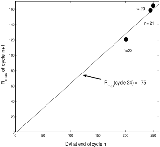
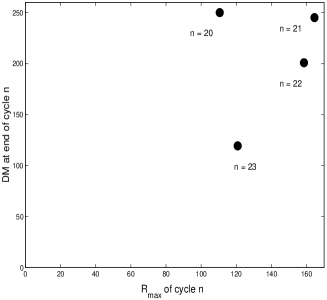
Figure 2: The left panel shows a plot of the strength of cycle $n+1$ against the polar field at the end of cycle $n$. The right panel shows a plot of the polar field at the end of cycle $n$ against the strength of the cycle $n$. From Choudhuri (2008).

We note another important thing in Fig. 1. The polar field at the end of cycle 22 was weaker than the polar field in the previous minimum. We see that this weaker polar field was followed by the cycle 23 which was weaker than the previous cycle. Does this mean that there is a correlation between the polar field during a sunspot minimum and the next sunspot cycle? In the left panel of Fig. 2, we plot the polar field in the minimum along the horizontal axis and the strength of the next cycle along the vertical axis. Although there are only 3 data points so far, they lie so close to a straight line that one is tempted to conclude that there is a real correlation. On the other hand, the right panel of Fig. 2, which has the cycle strength along the horizontal axis and the polar field at the end of that cycle along the vertical axis, has points which are scattered around. Choudhuri, Chatterjee & Jiang (2007) proposed the following to explain these observations. While an oscillation between toroidal and poloidal components takes place, the system gets random kicks at the epochs indicated in Fig. 3. Then the poloidal field and the next toroidal field should be correlated, as suggested by the left panel of Fig. 2. On the other hand, the random kick ensures that the toroidal field is not correlated with the poloidal field coming after it, as seen in the right panel of Fig. 2.

If there is really a correlation between the polar field at the minimum and the next cycle, then one can use the polar field to predict the strength of the next cycle (Schatten et al. 1978). Since the polar field in the just concluded minimum has been rather weak, several authors (Svalgaard, Cliver & Kamide 2005; Schatten 2005) suggested that the coming cycle 24 will be rather weak. Very surprisingly, the first theoretical prediction based on a dynamo model made by Dikpati & Gilman (2006) is that the cycle 24 will be very strong. Dikpati & Gilman (2006) assumed the generation of the poloidal field from the toroidal field to be deterministic, which is not supported by observational data shown in the right panel of Fig. 2. Tobias, Hughes & Weiss (2006) make the following comment on this work: “Any predictions made with such models should be treated with extreme caution (or perhaps disregarded), as they lack solid physical underpinnings.” While we also consider many aspects of the Dikpati–Gilman work wrong which will become apparent to the reader, we cannot also accept the opposite extreme viewpoint of Tobias, Hughes & Weiss (2006), who suggest that the solar dynamo is a nonlinear chaotic system and predictions are impossible or useless. If that were the case, then we are left with no explanation for the correlation seen in the left panel of Fig. 2.

Figure 3: A schematic cartoon of the oscillation between toroidal and poloidal components, indicating the epochs when the system is subjected to random kicks.

3 The flux transport dynamo model of the solar cycle

We now come to the theoretical question as to what causes the oscillation between the toroidal and poloidal components. Then in §4 we shall discuss how the random kicks shown in Fig. 3 arise.

The differential rotation of the Sun stretches any poloidal field line to produce a toroidal field, primarily in the tachocline where the differential rotation is strongest. Then this toroidal field rises due to magnetic buoyancy and produces sunspots (Parker 1955a). It is fairly easy to see how the toroidal field can be produced from the poloidal field. The production of the poloidal field from the toroidal field is more non-trivial. The original idea of Parker (1955b) and Steenbeck, Krause & Rädler (1966) was that the toroidal field is twisted by the helical turbulence in the convection zone giving rise to a field in the poloidal plane. This is, however, possible only if the toroidal field is not stronger than its equipartition value. Simulations based on the thin flux tube equation (Spruit 1981; Choudhuri 1990) suggest that the toroidal field is likely to be as strong as $10^{5}$ G at the bottom of the convection zone (Choudhuri 1989; D’Silva & Choudhuri 1993) and cannot be twisted by helical turbulence. We therefore invoke the alternate idea proposed by Babcock (1961) and Leighton (1969). We know that bipolar sunspots on the solar surface have tilts with respect to latitude lines, the leading sunspot appearing nearer the equator. Suppose we consider a pair in which the positive polarity sunspot is nearer the equator. When this pair decays, more positive polarity is spread around in lower latitudes and more negative polarity in the higher latitudes. This causes a poloidal magnetic field. A sunspot pair which forms from the toroidal field, therefore, acts as a conduit through which a conversion from the toroidal field to the poloidal field takes place. In a nutshell, the differential rotation acting on the poloidal field produces the toroidal field. The toroidal field, in turn, gives rise to the poloidal field by the Babcock–Leighton mechanism, thereby completing the cycle. However, a theoretical dynamo model with differential rotation and Babcock–Leighton mechanism alone gives rise to belts of toroidal field propagating poleward, in contradiction to the observation that the sunspots belts propagate equatorward. So we need something else. Choudhuri, Schüssler & Dikpati (1995), who pointed out this difficulty, also proposed a solution. They realized that the meridional circulation of the Sun can turn things around and can make the dynamo wave propagate in the correct direction.

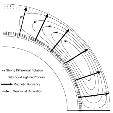
Figure 4: A cartoon explaining how the flux transport dynamo works.

Fig. 4 schematically shows the dynamo in which the meridional circulation plays a key role. Such a dynamo is often called a flux transport dynamo. First two-dimensional models of the flux transport dynamo were constructed by Choudhuri, Schüssler & Dikpati (1995) and Durney (1995), although the basic ideas were given in an early paper by Wang, Sheeley & Nash (1991). We now write down the basic equations of the flux transport dynamo. The axisymmetric magnetic field is represented in the form

$${\bf B}=B(r,\theta,t){\bf e}_{\phi}+\nabla\times[A(r,\theta,t){\bf e}_{\phi}],$$

where $B(r,\theta,t)$ and $A(r,\theta,t)$ respectively correspond to the toroidal and poloidal components. They evolve according to the equations

$$\frac{\partial A}{\partial t}+\frac{1}{s}({\bf v}.\nabla)(sA)=\eta_{p}\left(\nabla^{2}-\frac{1}{s^{2}}\right)A+\alpha B,$$

$$\frac{\partial B}{\partial t}+\frac{1}{r}\left[\frac{\partial}{\partial r}(rv_{r}B)+\frac{\partial}{\partial\theta}(v_{\theta}B)\right]=\eta_{t}\left(\nabla^{2}-\frac{1}{s^{2}}\right)B+s({\bf B}_{p}.\nabla)\Omega+\frac{1}{r}\frac{d\eta_{t}}{dr}\frac{\partial}{\partial{r}}(rB),$$

where $s=r\sin\theta$ and the other symbols have the usual meanings. Since nothing much can be done analytically, these equations have to be solved numerically. We have developed a code Surya, which we make available to anybody upon request. The right panel of Fig. 5, taken from Chatterjee, Nandy & Choudhuri (2004), shows the theoretical butterfly diagram superposed on a time-latitude plot indicating how $B_{r}$ evolves at the solar surface. The equatorward propagating meridional circulation at the bottom of the convection zone forces the sunspot belts to migrate equatorward, whereas the poleward propagating meridional circulation at the surface advects the poloidal field poleward. The right panel of Fig. 5 has to be compared with the comparable plot of observational data shown in the left panel. Given the fact that this was one of the first efforts of matching observational data in such detail, the fit is not too bad.

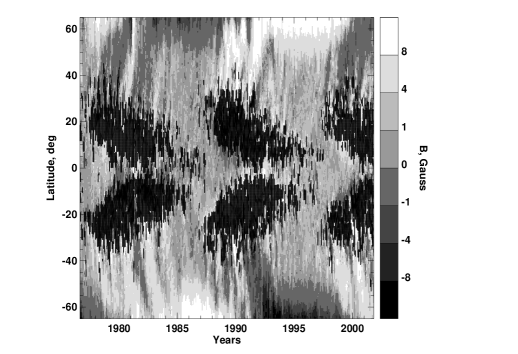
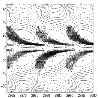
Figure 5: Butterfly diagram of sunspots superposed on the time-latitude plot of $B_{r}$. The observational plot is shown on the left. The comparable theoretical plot obtained by the dynamo model of Chatterjee, Nandy & Choudhuri (2004) is on the right.

The original flux transport dynamo model of Choudhuri, Schüssler & Dikpati (1995) led to two offsprings: a high diffusivity model and a low diffusivity model. The diffusion times in these two models are of the order of 5 years and 200 years respectively. The high diffusivity model has been developed by a group working in IISc Bangalore (Choudhuri, Nandy, Chatterjee, Jiang, Karak), whereas the low diffusivity model has been developed by a group working in HAO Boulder (Dikpati, Charbonneau, Gilman, de Toma). The differences between these models have been systematically studied by Jiang, Chatterjee & Choudhuri (2007) and Yeates, Nandy & Mckay (2008). Both these models are capable of giving rise to oscillatory solutions resembling solar cycles. However, when we try to study the variabilities of the cycles, the two models give completely different results. We need to introduce fluctuations to cause variabilities in the cycles. In the high diffusivity model, fluctuations spread all over the convection zone in about 5 years. On the other hand, in the low diffusivity model, fluctuations essentially remain frozen during the cycle period. Thus the behaviours of the two models are totally different on introducing fluctuations.

4 Modelling irregularities of solar cycles

Let us now finally come to question as to what produces the variabilities of cycles and whether we can predict the strength of a cycle before its advent. Some processes in nature can be predicted and some not. We can easily calculate the trajectory of a projectile by using elementary mechanics. On the other hand, when a dice is thrown, we cannot predict which side of the dice will face upward when it falls. Is the solar dynamo more like the trajectory of a projectile or more like the throw of a dice? Our point of view is that the solar dynamo is not a simple unified process, but a complex combination of several processes, some of which are predictable and others not. Let us look at the processes which make up the solar dynamo.

The flux transport dynamo model combines three basic processes. (i) The strong toroidal field is produced by the stretching of the poloidal field by differential rotation in the tachocline. (ii) The toroidal field generated in the tachocline gives rise to active regions due to magnetic buoyancy and then the decay of tilted bipolar active regions produces the poloidal field by the Babcock–Leighton mechanism. (iii) The poloidal field is advected by the meridional circulation first to high latitudes and then down to the tachocline, while diffusing as well. We believe that the processes (i) and (iii) are reasonably ordered and deterministic. In contrast, the process (ii) involves an element of randomness due to the following reason. The poloidal field produced from the decay of a tilted bipolar region by the Babcock–Leighton process depends on the tilt. While the average tilt of bipolar regions at a certain latitude is given by Joy’s law, we observationally find quite a large scatter around this average. Presumably the action of the Coriolis force on the rising flux tubes gives rise to Joy’s law (D’Silva & Choudhuri 1993), whereas convective buffeting of the rising flux tubes in the upper layers of the convection zone causes the scatter of the tilt angles (Longcope & Choudhuri 2002). This scatter in the tilt angles certainly introduces a randomness in generation process of the poloidal field from the toroidal field. Choudhuri, Chatterjee & Jiang (2007) identified it as the main source of irregularity in the dynamo process, which is in agreement with Fig. 3. It may be noted that Choudhuri (1992) was the first to suggest that the randomness in the poloidal field generation process is the source of fluctuations in the dynamo.

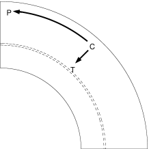
Figure 6: A sketch indicating how the poloidal field produced at C during a maximum gives rise to the polar field at P during the following minimum and the toroidal field at T during the next maximum. From Jiang, Chatterjee & Choudhuri (2007).

The poloidal field gets built up during the declining phase of the cycle and becomes concentrated near the poles during the minimum. The polar field at the solar minimum produced in a theoretical mean field dynamo model is some kind of ‘average’ polar field during a typical solar minimum. The observed polar field during a particular solar minimum may be stronger or weaker than this average field. The theoretical dynamo model has to be updated by feeding the information of the observed polar field in an appropriate way, in order to model particular cycles. Choudhuri, Chatterjee & Jiang (2007) proposed to model this in the following way. They ran the dynamo code from a minimum to the next minimum in the usual way. After stopping the code at the minimum, the poloidal field of the theoretical model was multiplied by a constant factor everywhere above $0.8R_{\odot}$ to bring it in agreement with the observed poloidal field. Since some of the poloidal field at the bottom of the convection zone may have been produced in the still earlier cycles, it is left unchanged by not doing any updating below $0.8R_{\odot}$. Only the poloidal field produced in the last cycle which is concentrated in the upper layers gets updated. After this updating, we run the code till the next minimum, when the code is again stopped and the same procedure is repeated. Our solutions are now no longer self-generated solutions from a theoretical model alone, but are solutions in which the random aspect of the dynamo process has been corrected by feeding the observational data of polar fields into the theoretical model.

Before presenting the results obtained with this procedure, we come to the question how the correlation between the polar field at the minimum and the strength of the next cycle as seen in the left panel of Fig. 2 may arise. This was first explained by Jiang, Chatterjee & Choudhuri (2007). The Babcock–Leighton process would first produce the poloidal field around the region C in Fig. 6. Then this poloidal field will be advected to the polar region P by meridional circulation and will also diffuse to the tachocline T. In the high diffusivity model, this diffusion will take only about 5 years and the toroidal field of the next cycle will be produced from the poloidal field that has diffused to T. If the poloidal field produced at C is strong, then both the polar field at P at the end of the cycle and the toroidal field at T for the next cycle will be strong (and vice versa). We thus see that the polar field at the end of a cycle and the strength of the next cycle will be correlated in the high diffusivity model. But this will not happen in the low diffusivity model where it will take more than 100 years for the poloidal field to diffuse from C to T and the poloidal field will reach the tachocline only due to the advection by meridional circulation taking a time of about 20 years. If we believe that the 3 data points in the left panel of Fig. 2 indicate a real correlation, then we have to accept the high diffusivity model!

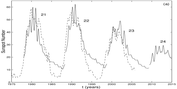
Figure 7: The theoretical monthly sunspot number (solid line) for the last few years as well as the upcoming next cycle, plotted along with the observational data (dashed line) for the last few years. From Choudhuri, Chatterjee and Jiang (2007).

Finally the solid line in Fig. 7 shows the sunspot number calculated from our high diffusivity model (Choudhuri, Chatterjee & Jiang 2007). Since systematic polar field measurements are available only from the mid-1970s, the procedure outlined above could be applied only from that time. It is seen from Fig. 7 that our model matches the last three cycles (dashed line) reasonably well and predicts a weak cycle 24.

5 Conclusion

It seems that the flux transport dynamo model explains many aspects of solar magnetism and probably will stand the test of time as the appropriate theoretical model for the solar cycle. In the recent past, two versions of the flux transport dynamo model have been developed in considerable detail: the high diffusivity version and the low diffusivity version. In the high diffusivity version, the poloidal field created at the surface by the Babcock–Leighton process is transported to the tachocline by diffusion. On the other hand, this transport is affected by the meridional circulation in the low diffusivity version of the flux transport dynamo. Several authors (Chatterjee, Nandy & Choudhuri 2004; Chatterjee & Choudhuri 2006; Jiang, Chatterjee & Choudhuri 2007; Goel & Choudhuri 2009; Hotta & Yokoyama 2010a, 2010b; Karak & Choudhuri 2010) have given several independent arguments in support of the high diffusivity model. This model has also been applied to provide theoretical explanations of such things as the helicity of active regions (Choudhuri, Chatterjee & Nandy 2004), the torsional oscillations (Chakraborty, Choudhuri & Chatterjee 2009) and the Maunder minimum (Choudhuri & Karak 2009). However, a crucial test of the high diffusivity model lies ahead. Since the high diffusivity model makes the polar field at a minimum correlated with the strength of the next cycle and the polar field during the immediate past minimum was weak, an inescapable conclusion of the high diffusivity model is that the upcoming cycle will be weak (Choudhuri, Chatterjee & Jiang 2007; Jiang, Chatterjee & Choudhuri 2007). While the early indications are that this will indeed be the case, we need to wait for a couple of years to be absolutely sure. If cycle 24 turns out to be strong as predicted by Dikpati & Gilman (2006), then there will be no way of reconciling that fact with the high diffusivity model and the model will have to be discarded. On the other hand, if cycle 24 turns out to be weak, that will provide a further corroboration of the high diffusivity model.

References

- [Babcock (1961)] Babcock, H. W. 1961, ApJ, 133, 572
- [Babcock & Babcock (1955)] Babcock, H. W., & Babcock, H. D. 1955, ApJ, 121, 349
- [Chakraborty et al. (2009)] Chakraborty, S., Choudhuri, A. R., & Chatterjee, P. 2009, Phys. Rev. Lett., 102, 041102
- [Charbonneau (2005)] Charbonneau, P. 2005 Living Rev. Solar Phys., 2, 2
- [Chatterjee & Choudhuri (2006)] Chatterjee, P., & Choudhuri, A. R. 2006, Solar Phys., 239, 29
- [Chatterjee et al. (2004)] Chatterjee, P., Nandy, D., & Choudhuri, A. R. 2004, A&A, 427, 1019
- [Choudhuri (1989)] Choudhuri, A. R. 1989, Solar Phys., 123, 217
- [Choudhuri (1990)] Choudhuri, A. R. 1990, A&A, 239, 335
- [Choudhuri (1992)] Choudhuri, A. R. 1992, A&A, 253, 277
- [Choudhuri (2008)] Choudhuri, A. R. 2008, J. Astrophys. Astron., 29, 41
- [Choudhuri et al. (2007)] Choudhuri, A. R., Chatterjee, P., & Jiang, J. 2007, Phys. Rev. Lett., 98, 131103
- [Choudhuri et al. (2004)] Choudhuri, A. R., Chatterjee, P., & Nandy, D. 2004, ApJ, 615, L57
- [Choudhuri & Karak (2009)] Choudhuri, A. R., & Karak, B. B. 2009, RAA, 9, 953
- [Choudhuri et al. (1995)] Choudhuri, A. R., Schüssler, M., & Dikpati, M. 1995, A&A, 303, L29
- [Dikpati & Gilman (2006)] Dikpati, M., & Gilman, P. A. 2006, ApJ, 649, 498
- [D’Silva & Choudhuri (1993)] D’Silva, S., & Choudhuri, A. R. 1993, A&A, 272, 621
- [Durney (1995)] Durney, B. R. 1995, Solar Phys., 160, 213
- [Goel & Choudhuri (2009)] Goel, A., & Choudhuri, A. R. 2009, RAA, 9, 115
- [Hathaway (2010)] Hathaway, D. H. 2010, Living Rev. Solar Phys., 7, 1
- [Hotta & Yokoyama (2010a)] Hotta, H., & Yokoyama, T. 2010a, ApJ, 709, 1009
- [Hotta & Yokoyama (2010b)] Hotta, H., & Yokoyama, T. 2010b, ApJ, 714, L308
- [Jiang et al. (2007)] Jiang, J., Chatterjee, P., & Choudhuri, A. R. 2007, MNRAS, 381, 1527
- [Karak & Choudhuri (2010)] Karak, B. B., & Choudhuri, A. R. 2010, arXiv:1008.0824v2
- [Leighton (1969)] Leighton, R. B. 1969, ApJ, 156, 1
- [Longcope & Choudhuri (2002)] Longcope, D. W., & Choudhuri, A. R. 2002, Solar Phys., 205, 63
- [Ossendrijver (2003)] Ossendrijver, M. A. J. H. 2003, A&AR, 11, 287
- [Parker (1955a)] Parker, E. N. 1955a, ApJ, 121, 491
- [Parker (1955b)] Parker, E. N. 1955b, ApJ, 122, 293
- [Schatten (2005)] Schatten, K. 2005, Geo. Res. Lett., 32, L21106
- [Schatten et al. (1978)] Schatten, K. H., Scherrer, P. H., Svalgaard, L., & Wilcox, J. M. 1978, Geo. Res. Lett., 5, 411
- [Spruit (1981)] Spruit, H. C. 1981, A&A, 98, 155
- [Steenbeck et al. (1966)] Steenbeck, M., Krause, F., & Rädler, K. H. 1966, Z. Naturforsch., 21, 369
- [Svalgaard et al. (2005)] Svalgaard, L., Cliver, E. W., & Kamide Y. 2005, Geo. Res. Lett., 32, L01104
- [Tobias et al. (2006)] Tobias, S., Hughes, D., & Weiss, N. 2006, Nature, 442, 26.
- [Wang et al. (1991)] Wang, Y.-M., Sheeley, N. R., & Nash, A. G. 1991, ApJ, 383, 431
- [Yeates et al. (2008)] Yeates, A. R., Nandy, D., & Mackay, D. H. 2008, ApJ, 673, 544