A Spitzer c2d Legacy Survey to Identify and Characterize Disks with Inner Dust Holes

Abstract

Understanding how disks dissipate is essential to studies of planet formation. However, identifying exactly how dust and gas dissipates is complicated due to difficulty in finding objects clearly in the transition of losing their surrounding material. We use Spitzer IRS spectra to examine 35 photometrically-selected candidate cold disks (disks with large inner dust holes). The infrared spectra are supplemented with optical spectra to determine stellar and accretion properties and 1.3mm photometry to measure disk masses. Based on detailed SED modeling, we identify 15 new cold disks. The remaining 20 objects have IRS spectra that are consistent with disks without holes, disks that are observed close to edge-on, or stars with background emission. Based on these results, we determine reliable criteria for identifying disks with inner holes from Spitzer photometry and examine criteria already in the literature. Applying these criteria to the c2d surveyed star-forming regions gives a frequency of such objects of at least 4% and most likely of order 12% of the YSO population identified by Spitzer.

We also examine the properties of these new cold disks in combination with cold disks from the literature. Hole sizes in this sample are generally smaller than for previously discovered disks and reflect a distribution in better agreement with exoplanet radii. We find correlations between hole size and both disk and stellar masses. Silicate features, including crystalline features, are present in the overwhelming majority of the sample although 10 µm feature strength above the continuum declines for holes with radii larger than $\sim$7 AU. In contrast, PAHs are only detected in 2 out of 15 sources. Only a quarter of the cold disk sample shows no signs of accretion, making it unlikely that photoevaporation is the dominant hole forming process in most cases.

1 Introduction

Near- and mid-IR observations of young stars demonstrate that optically-thick circumstellar disks disappear around approximately half of low-mass young stars in 1-3 Myr and are nearly entirely absent around members of 10 Myr old associations (e.g. Haisch et al. 2001; Gutermuth et al. 2004; Sicilia-Aguilar et al. 2005, Low et al. 2005; Currie et al. 2009). Accretion ceases on approximately the same timescale (e.g. Calvet et al. 2005). The disappearance of gas and dust - planetary building material - places stringent limits on the timescales of giant planet formation (Pollack et al., 1996; Kenyon & Bromley, 2009). However, identifying exactly how dust and gas dissipate is complicated due to the difficulty in identifying objects clearly in the transition of losing their surrounding material.

One of the most common methods, dating back to IRAS (e.g. Strom et al. 1989; Skrutskie et al. 1990), of identifying candidate transitional systems between the classical and debris disk evolutionary stages is through mid-IR spectral energy distributions (SEDs). Dust growth, sedimentation and removal is expected to result in a deficit of infrared flux as material is accreted or dispersed. This deficit has become the defining characteristic of transitional disks. For some disks, flux deficits are seen at all wavelengths, suggesting a gradual dissipation of mass for all disk radii. In other cases, a flux deficit is only seen at short wavelengths, indicating that the outer disk remains massive and optically thick while the inner disk lacks small dust grains. The presence of both types of transitional disks suggests that the transition happens via different paths from the gas-rich, optically-thick stage to gas-poor, optically-thin disks (Cieza et al., 2007; Currie et al., 2009). The fraction of stars with transitional disks is thought to be 5–25% (Lada et al., 2006; Hernández et al., 2007; Sicilia-Aguilar et al., 2008; Dahm & Carpenter, 2009; Currie et al., 2009; Kim et al., 2009). The small numbers indicate that the evolutionary path through a transitional disk is either uncommon or rapid. However, a consensus in nomenclature is still lacking: even within a single cluster, the calculated fraction of transitional disks can range from 10-50 %, depending on definitions (Ercolano et al. 2009; Sicilia-Aguilar et al. 2008).

Transition disks with a short wavelength deficit are particularly interesting because they are potential tracers of planet formation. This deficit arises from the absence of hot small dust grains close to the star resulting in flux coming solely from the stellar photosphere, rather than disk surface emission. This deficit may be the result of grain growth and sedimentation but also of complex interactions between a nascent protoplanet and the surrounding disk. The flux deficit from such inner holes results in a depressed SED at wavelengths less than $\sim$15 µm, while retaining typical fluxes at longer wavelengths from the outer disk. The short wavelength flux deficit arises from the absence of hot small dust grains close to the star resulting in flux coming solely from the stellar photosphere, rather than disk surface emission. We define such disks as “cold disks” to differentiate from other types of transitional systems (e.g. anemic or homologously depleted, defined as disks with an overall lower mass at all radii) and to emphasize that this is an observational characteristic not necessarily tied to evolution.

SEDs, relying heavily on mid-IR spectroscopy, are the tool currently most widely used to infer the presence of holes and gaps (e.g. Calvet et al. 2002; Forrest et al. 2004; Brown et al. 2007, hereafter B07). Additional submillimeter observations of the most massive disks have directly imaged large holes (Piétu et al., 2006; Hughes et al., 2007, 2009; Brown et al., 2008, 2009; Andrews et al., 2009). The hole sizes match reasonably well with estimates from SED modeling, suggesting that current interpretation and modeling of the SEDs is correct. Within the category of cold disks, significant differences are seen in hole sizes (from 1–50 AU), the presence or absence of gas and dust within the hole, and the presence or absence of accretion (Najita et al., 2007; Espaillat et al., 2007; Pontoppidan et al., 2008; Salyk et al., 2009; Kim et al., 2009). Detailed comparisons of these properties to the predictions of each of the scenarios listed above can help to discriminate which processes control the observed disk evolution. However, statistical studies (e.g. Najita et al., 2007) are limited by small sample sizes. Spitzer mapping efforts should include a significant number of unidentified cold disks and other types of transitional disks. However, accurately identifying these cold disks out of the large numbers of stars present in the maps is difficult with just broad band photometry. Reliable criteria for identifying disks with inner holes from Spitzer photometry, which lack any information on fluxes in the crucial region between 8 and 24 µm, are needed to generate a large sample for statistical purposes.

This paper presents a new large sample of cold disks identified from ‘Cores to Disks’ data (Evans et al., 2009) and analyzes simultaneously follow-up observations of the sample with the IRS and MIPS instruments together with optical spectroscopy and millimeter continuum observations. It is organized as follows: § 2 describes the target selection, observations and data reduction of the different data sets, including the Spitzer, optical spectroscopy and millimeter observations. The results are presented in § 3 and § 4, describing, in order, the stellar parameters in § 3, disk masses in § 4.1, the disk parameters in § 4.2 and the dust mineralogy in § 4.3 for the whole sample. Notes on individual sources are given in § 4.4. The combined analysis is presented at § 5, with first the presentation of a new selection criteria for transitional disks in § 5.1, then a description of the observational properties of our cold disks in § 5.2, and finally a discussion on the possible origins of the inner holes in § 5.3. The conclusions of this work are given in § 6.

2 Observations and data reduction

2.1 Target selection

The c2d Spitzer Legacy program completed a full IRAC (3.6 to 8 $\mu$m) and MIPS (24 to 160 $\mu$m) survey of five nearby star-forming regions (Perseus, Chameleon II, Lupus, Ophiuchus, and Serpens) (Evans et al., 2003; Jørgensen et al., 2006; Alcalá et al., 2008; Merín et al., 2008; Harvey et al., 2007). From these maps, 1024 Young Stellar Object (YSO) candidates were identified using the selection techniques, including removing extragalactic contaminants, described in Harvey et al. (2007) (see Evans et al. 2009 for a complete description of this sample and a general study of cloud to cloud differences). This sample should include a significant number of cold disks but they must first be separated from the bulk of the population.

Cold disks were selected for IRS follow-up using the following method. Spectral types were taken from the literature where possible or otherwise a K7 photosphere was used to get an initial estimate of the SED. Sources with photospheric fluxes in at least IRAC 1 (3.6 $\mu$m) and IRAC 2 (4.5 $\mu$m) and 24 $\mu$m excesses equal or greater than IRAC 4 (8.0 $\mu$m) fluxes in $\lambda$F_λ space were selected. Sources with rising or flat SEDs from 8 $\mu$m to 24 $\mu$m were preferentially included. A flux lower limit of 15 mJy at 8 $\mu$m was imposed to further reduce extragalactic contamination and keep integration times reasonable. The initially selected sample was then cut slightly to reject likely contaminants and to avoid overlap with other IRS programs. A total of 33 sources were selected in this fashion. To further expand our sample, two additional candidate cold disks within the c2d clouds were included from a survey of Weak Line T Tauri stars (WTTs, Padgett et al. 2006; Cieza et al. 2007) based on their IRS spectra suggestive of inner holes. In total, 35 objects were included in our sample and followed-up with IRS and MIPS (§ 2.2), optical spectroscopy (§ 2.3), and millimeter continuum observations (§ 2.4).

2.2 Spitzer IRS and MIPS observations

Spectra for the 35 objects in Table 1 were obtained using the Infrared Spectrograph (IRS) aboard the Spitzer Space Telescope under a variety of programs. Most were observed as part of program 30843 (P.I.: B. Merín), which also included deep 70 $\mu$m MIPS staring observations of the same sample. Objects 17 and 19 were observed with IRS as part of the c2d second look observations of WTTs from Padgett et al. (2006) and object 25 was observed during the IRS Guaranteed Time Observation (GTO) although it was selected as a candidate from the c2d photometry. All the candidate cold disks in Serpens were observed as part of a complete flux-limited IRS survey in Serpens, program 30223 (P.I.: K. Pontoppidan) and will also be discussed along with the rest of the Serpens sample in Oliveira et al. (2010). Table 1 gives the AORs and observing dates for both the IRS and MIPS-70 observations of the sample.

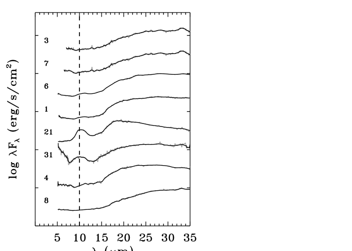
Figure 1: IRS spectra of the of the close to edge-on systems ordered from bottom to top with growing effective temperature. The thick and grey lines are the binned and original spectra, respectively and the numbers give their identifications in Table 1.

All the IRS spectra were obtained with a combination of Short-Low (SL) and Long-Low (LL) modules, which provide a resolving power of $R=\Delta\lambda/\lambda\sim 100$ and a combined wavelength coverage from 5.3 to 35.0 $\mu$m. Integration times were estimated from the IRAC flux at 8 $\mu$m and MIPS flux at 24 $\mu$m. The observations typically ranged from 5 to 20 minutes, resulting in signal to noise values of 30 to 150, depending on the background level and the brightness of the objects. Given the rising SED of the targets at long wavelengths, longer times were usually needed in the SL than LL observations. The observations were scheduled in cluster mode, grouping nearby sources with similar integration times to increase the observing efficiency. Data reduction started from the Basic Calibrated Data (BCD) images, pipeline version S12.4.0. The processing includes bad-pixel correction, extraction, defringing, and order matching using the c2d analysis pipeline (Kessler-Silacci et al. 2006, see also the c2d Spectroscopic Explanatory Supplement, from the SSC webpage). The final spectra can be found in Figures 1 to 5.

The same clustering strategy was used for the MIPS observations at 70 $\mu$m. The integration times were set to 300 seconds, with achieved sensitivities given in Table A Spitzer c2d Legacy Survey to Identify and Characterize Disks with Inner Dust Holes. The small maps were reduced following the procedure described in Cieza et al. (2008a) and using the SSC median-filtered BCDs from the SSC pipeline version S16.1.0. Details of the method can be found in the aforementioned paper, but in short, the photometry is determined with an aperture of 16^′′ radius and a sky annulus with inner and outer radii of 48^′′ and 80^′′, respectively. Visual inspection and correction factors suggested by the SSC were used in all cases. The resulting fluxes are given in Table A Spitzer c2d Legacy Survey to Identify and Characterize Disks with Inner Dust Holes, together with the other IRAC and MIPS fluxes from c2d.

2.3 Optical Spectroscopy

Optical spectra were obtained for 21 objects in our sample using the Wide Field Fibre Optical Spectrograph (WYFFOS, Bingham et al. 1994) on the 4.2m William Herschel Telescope (WHT), the Intermediate dispersion Spectrograph and Imaging System (ISIS) at the WHT, the Intermediate Dispersion Spectrograph (IDS) at the Isaac Newton Telescope (INT, see Carter et al. 1994 for a description of last three instruments), the Calar Alto Faint Object Spectrograph (CAFOS) at the 2.2m Calar Alto Telescope, the Double Spectrograph (DBSP, Oke & Gunn 1982) at the 5m Hale Telescope at Palomar Observatory, and with the R-C Spectrograph on the 1.5m CTIO telescope. These observations typically cover $\sim 5500-8500$ Å with a resolving power of $\sim 1000-5000$. Table 3 lists the instrument setups and observation log.

Data were reduced and spectra were extracted using standard methods in IDL and IRAF. No telluric correction or flux calibration was performed. For WYFFOS, a fiber-fed multi-object spectrograph, sky subtraction was obtained from fibers that were placed on blank sky regions (see Oliveira et al. 2009 for details).

2.4 IRAM-30 millimeter observations

A subsample of 17 of the northern targets was observed with the IRAM-30m telescope in Pico Veleta. The observations were carried out with MAMBO-2 (Kreysa et al., 2002) mounted on the IRAM-30m Telescope during the 2007 winter and summer pool sessions. MAMBO-2 is a 117-bolometer array with a half-power spectral bandwidth of 80 GHz centered on $\sim$ 250 GHz (1.2 mm), yielding a beam size of 11^′′. The data were analysed with the MOPSI software (Zylka, 1998). The flux calibration was performed by observing either Mars or Uranus to determine the flux conversion factor. For each channel the sky noise was subtracted by computing the weighted mean of the signals from the surrounding six channels.

All Perseus sources from our sample (see Table 1) were observed, except numbers 3, 6, 8 and 11. We also observed sources 20, 21 and 22 in Ophiuchus and sources 33, 34 and 35 in Serpens. The ON/OFF observing mode was used with a throw of 35^′′ and each source was observed until a $>3\sigma$ detection was obtained, or until an rms of 0.7 mJy (whenever possible) was reached. The integration times ranged from 10 to 40 minutes. In general, the sky noise of the array was low ($<80$ mJy), and was never larger than $\sim$ 100 mJy. Ten sources were detected with fluxes between 1 and 10 mJy, while the other 7 have upper limits between 1 and 7 mJy. These fluxes can be found in column 8 of Table A Spitzer c2d Legacy Survey to Identify and Characterize Disks with Inner Dust Holes.

3 Stellar Properties

Stellar properties must be determined to understand and interpret data on the surrounding disks. Optical spectra are used here to measure spectral types and to determine whether accretion is ongoing. We obtained optical spectra for 21 of the 35 objects in our sample. Of the other 14 stars, 11 have published spectral types and accretion properties. For the remaining three sources, spectral types are estimated from an SED analysis of broadband photometry and accretion properties are left uncertain. The SED fits are also used to measure the extinction to each source. Results are presented in Table A Spitzer c2d Legacy Survey to Identify and Characterize Disks with Inner Dust Holes.

For the 21 objects for which we obtained optical spectra, spectral types of G and K stars were assigned by finding a best match to the depth of photospheric absorption features in template spectra obtained from the EXPORT spectral library (Mora et al., 2001). Spectral types of M-dwarfs were assigned by finding the best match to the TiO absorption bands from template spectra (Montes et al., 1997). The uncertainty in SpT is typically $\sim 3$ subclasses for G and K stars and $1$ subclass for M stars. Object 6 is classified as a continuum object because no spectral features were detected in the low-resolution spectrum. Any possible optical veiling was not considered for the other objects in the sample. A more detailed description of our spectral typing and the stellar properties of all the Serpens objects are presented by Oliveira et al. (2009). Literature values for SpT are adopted for several objects that we did not observe and for several objects where the literature SpT is more reliable than the SpT from our spectra. Spectral types are converted to $T_{eff}$ using the scales in Kenyon & Hartmann (1995) for objects earlier than M0 and Luhman et al. (2003) for those later or equal to M0, to account for the lower surface gravity atmosphers of mid M stars.

The extinction and luminosity for each object were calculated using SED fits to broadband optical and near-IR photometry (see Table A Spitzer c2d Legacy Survey to Identify and Characterize Disks with Inner Dust Holes for photometry and § 4.2 for a discussion on the assumed extinction law). Assumed distances are listed at the bottom of Table A Spitzer c2d Legacy Survey to Identify and Characterize Disks with Inner Dust Holes. NEXTGEN models of stellar photospheres (Hauschildt et al., 1999) are used as templates for the broadband emission. The 2MASS and any optical photometry are the primary constraints on extinction and stellar luminosity. For the 3 objects that lack optical spectra (identified with a “2” in Table A Spitzer c2d Legacy Survey to Identify and Characterize Disks with Inner Dust Holes), the SED fits are also used to estimate SpT. However, these SpT estimates have large uncertainties because they are based on JHK colors, which are not very sensitive to spectral types from mid-K through M (Leggett 1992; Kenyon & Hartmann 1995).

Stellar ages and masses are estimated by comparing the stellar luminosity and effective temperature to pre-main sequence tracks of Baraffe et al. (1998) for low-mass stars ($<1.4$ $M_{\odot}$, mixing length = 1) and Siess et al. (2000) for higher-mass stars. Since uncertainties in stellar age are large they are not tabulated here and we focus the analysis on the better constrained stellar masses.

3.1 Edge-on Disks

In the process of determining the stellar properties, it became clear that a fraction of the sample sources were actually edge-on disks. Inferring disk structure from an SED analysis is difficult when the disk is viewed edge-on and occults the star. In these cases, optical and near-IR light from the star and inner disk are only seen in reflected emission (e.g. Padgett et al., 1999). The strength of such emission depends on the precise viewing angle and the disk flaring, but is always much fainter than it would be if the disk were viewed without the large absorption column from the edge-on disk. Emission from outflows, seen prominently in optical forbidden lines, are not occulted by the disk and can therefore have large equivalent widths (White & Hillenbrand, 2004).

Based on the existing data on our sources, we establish four criteria to determine whether a disk is viewed edge-on: (1) a low ratio of photospheric luminosity to main-sequence luminosity, assessed at $10^{8}$ Myr from Baraffe et al. (1998); (2) large equivalent widths in optical forbidden lines; (3) strong silicate and/or ice absorption in the IRS spectra; and (4) high infrared luminosity compared to stellar luminosity. Any one of these criteria can be degenerate between edge-on disks and other explanations, due to potential errors in distance and extinctions and the absence of accretion/outflow activity. However, the presence of at least two of these four criteria should establish in most cases that the disk is edge-on. Eight of the sources were selected as edge-on disks and the reasons are marked in Table 6. No further analysis was done on these disks as the stellar properties are too uncertain.

3.2 Accretion Properties

The presence or absence of accretion can be assessed from the strength and shape of emission in several optical lines, most prominently H$\alpha$. Though some H$\alpha$ emission is produced in chromospheres of late-type stars, accretion typically generates H$\alpha$ emission with much larger equivalent widths and broader spectral profiles (see Hartmann 2001 for a comprehensive description of accretion phenomenology and diagnostics). A 10 Å cutoff in equivalent width has historically been used to identify accretion, though this rough cutoff depends on spectral type (White & Basri 2003; Fang et al. 2009). More recently, the H$\alpha$ 10% width (defined as the full width of the H$\alpha$ line at 10% of the peak flux) has been used to discriminate between accretors and non-accretors (White & Basri 2003; Muzerolle et al. 2003; Jayawardhana et al. 2006). Accretion/outflow activity can also produce asymmetries and absorption components within the line profile (e.g., Reipurth et al. 1996, Muzerolle et al. 2003, Kurosawa et al. 2006) and variable line fluxes and shapes (e.g., Nguyen et al. 2009). For any such criteria, a small accretion rate relative to the stellar luminosity is not detectable.

To classify the accretion properties of stars in our optical sample, a Gaussian profile is fit to the H$\alpha$ line. We then measure the equivalent width and, when possible, the H$\alpha$ 10% width from the Gaussian profile, after accounting for the resolution of each observation (see a more complete discussion of this method in Oliveira et al. 2009). Uncertainties in H$\alpha$ 10% widths range from 50–150 km s^-1. The H$\alpha$ equivalent width and 10% width are then used together with the spectral type to assess whether accretion is ongoing, adhering to the loose guidelines suggested by White & Basri (2003) and Fang et al. (2009). Typically, a star is classified an accretor if the H$\alpha$ 10% width is $>300$ km s^-1 and the H$\alpha$ equivalent width is $>3$ Å for an early K star, $>10$ Å for late K star and $>20$ Å for an M star.

We classify 21 stars in our sample as accretors and 8 stars as non-accretors, with 6 cases lacking information. In many cases an object is clearly accreting. As explained below, some classifications are ambiguous both because some accretors and non-accretors have similar H$\alpha$ 10% and equivalent widths and because the uncertainties in H$\alpha$ 10% width are large. Objects 23 and 24 have weak H$\alpha$ equivalent widths but broad H$\alpha$ line shapes. Such observations could be explained if accretion is present with strong absorption, either from outflows or the accretion flow itself, that suppresses the H$\alpha$ emission (e.g. Reipurth et al. 1996), if the star is an unresolved binary with only one accreting component, or if the stars are chromospherically active with large $v$ sin $i$ (Jayawardhana et al., 2006). The highest-resolution spectrum of object 24 shows absorption in H$\alpha$, while two of the three show [O I] in emission. This star is therefore classified as an accretor. On the other hand, object 23 shows no other evidence of accretion and is classified as a non-accretor. Object 18 is left unclassified because the H$\alpha$ equivalent width is ambiguous between accretion and non-accretion. The H$\alpha$ emission from DoAr 21 (object 25) has varied on long timescales, but with no definitive evidence for accretion (Jensen et al., 2009). Temporal variations in H$\alpha$ also introduce uncertainty in classifying the presence or absence of accretion. A mass-dependent bias likely exists in this classification scheme because the stronger photospheric continuum emission and spectral type degeneracy for stars with early spectral types can mask H$\alpha$ emission produced by weak-to-moderate accretion onto the star. Based on these uncertainties, we suspect a small number of objects in our sample (estimated at $<$10%) might be misclassified as accretors or non-accretors.

To quantify accretion, we convert the H$\alpha$ 10% widths to accretion rate using the relationship derived by Natta et al. (2004). Methodological differences in measuring the H$\alpha$ 10% width between this work and Natta et al. (2004) likely leads to an order-of-magnitude uncertainty in the listed accretion rates. For late-K and early M-dwarfs, which comprise the bulk of our sample, the H$\alpha$ 10% width is not sensitive to accretion rates $<10^{-10}$ $M_{\odot}$ yr^-1. For earlier spectral types, the sensitivity worsens to larger accretion rates. Table A Spitzer c2d Legacy Survey to Identify and Characterize Disks with Inner Dust Holes gives the H$\alpha$ equivalent widths, 10 % widths and mass accretion rates derived from this work and Table 8 gives the final classification of each source.

4 Results: Disk and Disk Hole Parameters

4.1 Disk mass

Millimeter continuum fluxes can be used to calculate disk masses assuming that the millimeter emission is optically thin and a gas to dust mass ratio of 100. The disk masses can then be used in turn to constrain SED models. The disk masses, $M_{\rm Disk}$, are calculated following Beckwith et al. (1990) and with standard assumptions and parameters. In the Rayleigh-Jeans limit,

$$M_{\rm Disk}={F_{\nu}}\frac{d^{2}}{2k<T>}\frac{c^{2}}{\nu^{2}\kappa_{\nu}},$$ (1)

where ${F_{\nu}}$ is the flux at frequency $\nu$, here 230 GHz, $d$ is the distance to the star (see Table A Spitzer c2d Legacy Survey to Identify and Characterize Disks with Inner Dust Holes), $k$ is the Boltzmann constant, and $\kappa_{\nu}$ is the opacity. It is assumed that the emission arises primarily from an approximately isothermal region with temperature, $<$$T$$>$. Average disk temperatures in the outer disk range from 10 to 50 K and here we have used 30 K. One of the major uncertainties is the opacity, $\kappa_{\nu}$. We follow Beckwith et al. (1990) and adopt $\kappa_{0}$ = 0.02 cm²g^-1 anchored at $\nu_{0}$ = 230 GHz, the frequency of our observations.

Disk masses are listed in Table A Spitzer c2d Legacy Survey to Identify and Characterize Disks with Inner Dust Holes for the ten detected sources and the seven with upper limits. The majority (80%) of the disks in our sample have disk masses of less than 2 $\times$ 10^-3 M_⊙ and the sample has an average $M_{\rm Disk}$ of 4.5${}^{+5.5}_{-1.4}\times 10^{-3}$ M_⊙. These are relatively low mass disks compared to many millimeter studies, such as the large sample of T Tauri disks in Andrews & Williams (2007) which have an average mass of 10^-2 M_⊙ using the same assumptions.

4.2 Disk hole parameters from SED modeling

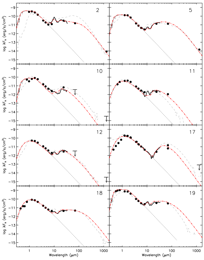
Figure 7: Spectral Energy Distributions of the disks with holes in the sample. Points are dereddened fluxes from IRAC, MIPS and IRAM. The thick solid line is the IRS spectrum, the dotted line is the stellar photospheric model, the red dash-dot line is the best-fit RADMC disk model, and the thin black dashed line is the Robitaille model fit. The numbers give their identifications in Table 1.

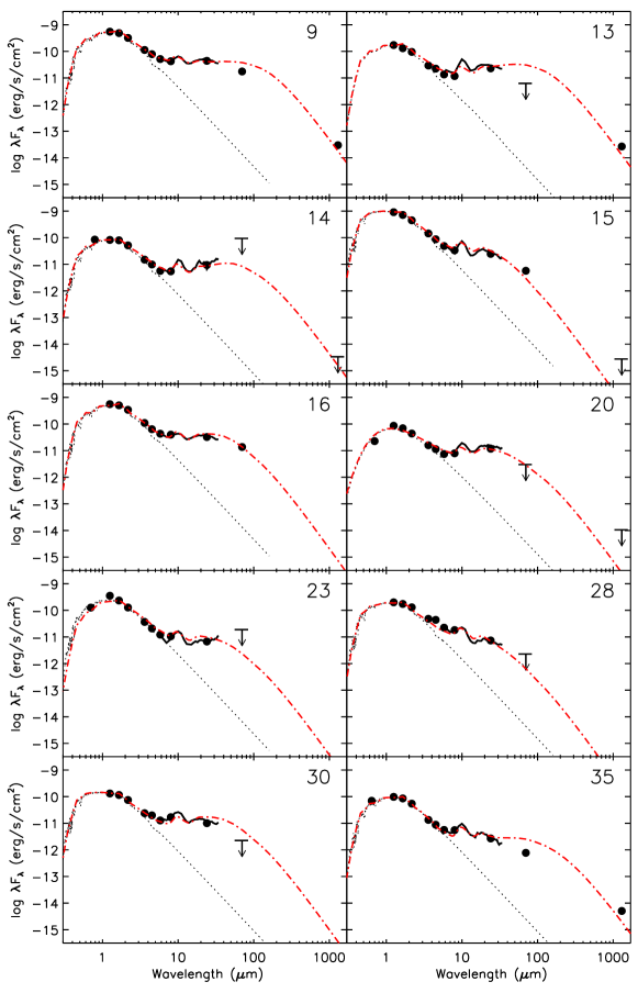
Figure 9: Spectral Energy Distributions of the disks without holes in the sample. Points are dereddened fluxes from IRAC, MIPS and IRAM. The thick solid line is the IRS spectrum, the dotted line is the stellar photospheric model and the red dash-dot line is the best-fit RADMC disk model. The numbers give their identifications in Table 1.

In order to determine the presence or absence of a hole, the full SED is needed to determine the disk structure. The SEDs for the stars in the sample are organized by type with edge-on disks (Figure 6), disks with holes (Figure 7 and 8), and disks without holes (Figure 9). The solid dots are dereddened fluxes, which contains the 2MASS JHK fluxes, the 4 IRAC fluxes from 3.6 to 8 $\mu$m and the MIPS fluxes at 24 and 70 $\mu$m for all sources, plus optical or 1.3mm fluxes for a smaller subsample of the objects. In some cases, 70 µm  photometry produced only upper limits, often accompanied by non-detections at 1.3mm, and thus severely limits information about the outer disk. The solid dots are the dereddened fluxes, the solid line is the IRS spectrum binned at a resolution of 1 µm, the grey dotted line is the stellar Kurucz model of the central star. The differences between the Kurucz and the NEXTGEN stellar models used above are negligible for the purposes of disk characterization.

The data were dereddened using the $A_{\rm V}$ values listed in Table A Spitzer c2d Legacy Survey to Identify and Characterize Disks with Inner Dust Holes and the extinction law by Weingartner & Draine (2001) with $R_{V}$=5.5. Recently, Evans et al. (2009) and Chapman et al. (2009) have suggested that this larger value of $R_{V}$ is more suitable for star forming clouds than the typical value of $R_{V}$=3.1, which is based on models and observations of the diffuse interstellar medium. The higher $R_{V}$ value reflects larger maximum dust grain sizes and results in stronger dereddening effects throughout the mid-IR. Dereddened fluxes are 2-4 times higher at 24 µm  and $A_{V}>$10 than with $R_{V}$=3.1. However, observational measures of extinction indicate that the large amount of reddening is in agreement with observations and may even underestimate the actual effect in star forming regions (Chapman et al. 2009; Flaherty et al. 2007).

As the extinction law is not flat throughout the mid-IR, errors in the mid-IR extinction law could potentially artificially create or remove SED deficits mimicking inner holes. Corrections are much smaller at low $A_{V}$, so effects only become significant for $A_{V}>$ 10. Based on observations, the extinction law used here is conservative with some cold disks being potentially missed due to inadequate dereddening around 20 µm. With such large grain sizes in the absorbing dust, silicate grain opacities are expected to have strong effects on the 10 µm  silicate feature. In a few dereddened SEDs, strong silicate features are seen which are not present in the uncorrected spectra. The effects of extinction on the silicate features are complex and dependent on extinction and line-of-sight ice and dust composition, which may not be uniform throughout star forming regions (McClure, 2009). Due to this uncertainty, all work on the silicate feature in this paper has been done on spectra which have not been dereddened, with the caveat that sources with high $A_{V}$ have large errors (see also discussion in Oliveira et al. 2010).

The 2-D radiative transfer model RADMC (Dullemond & Dominik, 2004), as modified to include a density reduction simulating a hole, was used to model the SEDs. The model has a large number of input parameters and we have fixed as many as possible. The model assumes a passive disk, which merely reprocesses the stellar radiation field and does not account for accretion luminosity and heating. This is justified since the disk to stellar luminosity ratios of the majority of the disks in this study are below 0.4 (see Table A Spitzer c2d Legacy Survey to Identify and Characterize Disks with Inner Dust Holes). Further discussion on the disk model dependency of the results can be found in § 5.2. Stellar input parameters are mass, temperature and luminosity which were determined from optical spectroscopy and photospheric SED fits (see Table A Spitzer c2d Legacy Survey to Identify and Characterize Disks with Inner Dust Holes). A stellar Kurucz model is then used for the stellar radiation field. In terms of disk structure, the disk is assumed to be flared such that the surface height, $H$, varies with radius, $R$, as $H/R\propto R^{2/7}$, as in Chiang & Goldreich (1997). The models do not calculate the hydrostatic equilibrium self-consistently allowing the dust distribution to differ from the gas distribution (expected to be in hydrostatic equilibrium) due to effects such as dust settling. The pressure scale height is anchored at the outer disk edge, in this case 200 AU. In some cases, some degree of settling appears to have taken place. We present this number as a fraction of the scale height predicted from hydrostatic equilibrium, assuming a midplane temperature of 20 K. In cases where the disk has settled, a flaring index of 2/7 (0.29) is likely too large (see e.g. Andrews et al. 2009 where flaring indices range from 0.04 to 0.26). Disk model SEDs with large flaring indices are similar to cold disk SEDs in having more flux at longer wavelengths. By using a large flaring index as our default, we are more conservative when reporting the presence of a hole. Surface density is a power law of radius with an index of -1 inside 200 AU and then steepens to an index of -12 outside the 200 AU outer disk edge. The dust composition is set to a silicate:carbon ratio of 3:1 with only amorphous, as opposed to crystalline, silicate included. Silicate opacities were taken from Beckwith et al. (1990) which provides opacities into the millimeter. Disk masses were taken from 1.3mm observations where possible (see Table A Spitzer c2d Legacy Survey to Identify and Characterize Disks with Inner Dust Holes) and left as a free parameter otherwise. Disk mass and disk settling are highly degenerate parameters in the absence of (sub)millimeter fluxes, so when the disk mass is unknown, the scale height is left at the hydrostatic value (see note on exception for sources 18, 19 and 24 in Section 4.4). As a result, model-derived disk masses tend to be systematically small and together with observational upper limits provide a range of likely disk masses. The inner edge of the disk, when no hole is present, was set at approximately the radius where the dust sublimation temperature, 1500 K, is reached. Some cold disks in the literature have near-infrared excesses most easily modelled as a gap rather than a hole (e.g. Brown et al. 2007; Espaillat et al. 2008). However, none of the sources in this sample required warm dust within the hole. Those sources which did have some near-infrared excess turned out to be compatible with disk models without holes. The hole is represented in the model by a hole radius, $R_{\rm Hole}$ and a density reduction, set here to a factor of 10^-6, providing an almost entirely clean hole. Thus, the four free parameters are $R_{\rm Hole}$, degree of settling, disk inclination and disk mass when there are no measurements.

A two step procedure was used to find the best model fits. First, we ran a large grid of disk models with a broad range of disk and hole parameters and a limited number of stellar templates. Then, we ran a finer grid of disk and hole parameters, determined from the larger grid, for each individual star using the stellar properties in Table A Spitzer c2d Legacy Survey to Identify and Characterize Disks with Inner Dust Holes. A simple $\chi^{2}$ minimization was performed at each step between the dereddened SEDs and the model SEDs and the resulting best fit is shown as a red dash-dot line in the SED plots (Figures 7 and 9). Errors on the hole radii are given in Table A Spitzer c2d Legacy Survey to Identify and Characterize Disks with Inner Dust Holes based on fits with up to 20% deviation in $\chi^{2}$.

Fifteen of the 25 modelled stars require inner holes while the remaining 10 require no hole to fit the SED. The 10 sources not modelled are the 8 edge-on disks and 2 sources, 25 and 27, which have strong extended 70 µm  emission and cannot be fit with disk models (see section 4.4 for further details). Hole radii range from 1 AU to 55 AU. Holes smaller than 1 AU cannot be firmly identified. The range of hole radii can be seen in histogram form in Figure 11.

In order to confirm our results above and identify the less model-dependent part of our results, we also fitted our sample SEDs with the on-line SED fitting tool by Robitaille et al. (2007). This system offers the possibility of fitting young star SEDs with a precomputed grid of 200,000 synthetic SEDs from stars, disks and envelopes with a broad range of physical parameters. In order to make these fits, we observed photometry from Table A Spitzer c2d Legacy Survey to Identify and Characterize Disks with Inner Dust Holes and A Spitzer c2d Legacy Survey to Identify and Characterize Disks with Inner Dust Holes along with a binned IRS spectrum in from 6 to 33 $\mu$m with steps of 1 $\mu$m. An aperture of 4.5 arcsec, a distance range from 0.1 to 0.33 kpc and a A_V range from 0 to 30 mags were used in all fits. For the objects for which the spectral types are known, we select the best fitting model with an effective temperature less than 500 K away from the target’s one. The final best-fit models used are good representation of the median properties of the best fitting models with the appropriate effective temperatures but should not be considered as definitively constrained parameters.

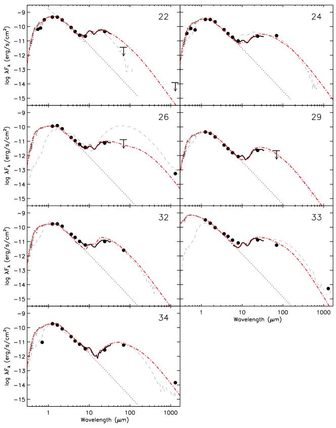
Figure 8: Figure 7 continued.

Figures 7 and 8 show the Robitaille et al. best-fit models for the objects in our sample as thin black dashed lines and Table A Spitzer c2d Legacy Survey to Identify and Characterize Disks with Inner Dust Holes shows their corresponding model ID’s and the inner disk radii in the cases where it is clearly distinguishable from the dust destruction radius disk inner radius. In order to overplot the Robitaille et al. models, we corrected them with the extinction law given in the web-fitting tool and using the total A_V value given by the best-fit model and normalized it to the $K_{\rm 2MASS}$-band dereddened flux. The $A_{V}$ values of the best-fit models used are in general in agreement with the $A_{V}$ values obtained from the spectral type and optical photometry. However, small discrepancies plus small differences in the standard extinction laws used to deredden our photometry and the Robitaille models can explain the discrepancies between the Robitaille models and optical fluxes in some cases.

All but source 18 of the cold disks in Figure 7 also have inner holes with the Robitaille et al. models. The only exception, source 18, is a border-line case with an extremely small inner cavity of 0.03 AU in the Robitaille et al. best-fit model. On the other hand, almost all the objects in Figure  9, which have no hole according to the RADMC models, show inner cavities smaller than 2 AU in the Robitaille models. The only exception is source 15, which is also among the flattest disk in the group. This indicates that in general terms, the classification of objects as disks with or without inner holes is model independent as long as the disk hole is larger than 2 AU.

Figure 10 compares the disk inner holes estimated both with the RADMC and the Robitaille et al. (2007) disk model grids. The plot does not include the only outlier (Source 18). For the rest of the sample, the values from both sets of models are correlated, but with a very large scatter. It must be noted that this comparison is not straight forward as both sets of models have different treatments of the dust opacities, disk flaring angle, and inner hole structure. Also, the Robitaille et al. on-line tool does not allow the use of a priori information like the lack of an envelope, or the effective temperature of the central star, both of which have obviously great impact on the final result of the fitting. Pursuing a more detailed comparison between both sets of disk models is beyond the scope of this paper but this comparison shows that the derived disk hole radius is model independent to within a factor of 2-3 generally. We find the RADMC models more reliable due to the greater control over the input parameters and the resulting better fits. The RADMC disk radii are therefore used in all further comparisons.

4.3 Dust composition

A wide variety of mid-infrared spectral features have been detected in spectra of disks around low- and intermediate mass young stars using ISO (e.g., Acke & van den Ancker 2004) and Spitzer (e.g., Kessler-Silacci et al. 2006; Furlan et al. 2006; Lahuis et al. 2007; Bouwman et al. 2008; Watson et al. 2009; Olofsson et al. 2009). These features can serve as diagnostics of physical processes in disks such as grain growth, fragmentation, crystallization, flaring, and UV or X-ray illumination. An interesting question is whether the spectral features of cold disks differ significantly from those of normal T Tauri disks, and if so, what that tells us about the disk structure and evolution.

Table 8 identifies the presence or absence of the 10 and 20 $\mu$m silicate emission features, PAHs and crystalline silicate features, where ”Y” means a detection, ”N” a non-detection and ”T” a tentative detection. The spectra presented in Figures 1 to 5 clearly show a large variety of features in our sample of cold disks.

4.3.1 Silicates

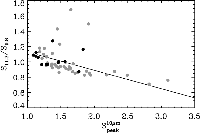
Figure 13: Shape-strength diagram for the 10 $\mu$m silicate emission feature for all cold disks in this sample (filled dots), compared with those of the c2d IRS T Tauri sample (Olofsson et al. 2009, grey dots).

The silicate 10 and 20 $\mu$m features are detected in most cases; none of the sources show the featureless spectra commonly seen for older (debris) disks (e.g., Jura et al. 2004; Chen et al. 2006; Carpenter et al. 2009). However, only a few sources have pristine ISM-like 10 $\mu$m silicate features, characterized by a strongly peaked profile centered at 9.8 $\mu$m. This is illustrated in Figure 13, in which the $S_{11.3}/S_{9.8}$ $\mu$m flux ratio is plotted versus the strength of the feature above the continuum $S^{10\mu m}_{\rm peak}$, as defined in Kessler-Silacci et al. (2006). The different quantities $S_{11.3}$, $S_{9.8}$ and $S_{\mathrm{Peak}}^{10\mu m}$ are calculated after normalizing the observed feature as follows $S_{\nu}=1+(F_{\nu}-F_{\nu,\mathrm{cont}})/(<F_{\nu,\mathrm{cont}}>)$, where $F_{\nu,\mathrm{cont}}$ is the local continuum and $<F_{\nu,\mathrm{cont}}>$ the mean value of this continuum. The local continuum is estimated using a second degree polynomial, normalized at 6.8–7.5 $\mu$m, 12.5–13.5 $\mu$m and 30–36 $\mu$m. The fluxes are measured as an averaged flux of the continuum-subtracted spectra in a $\pm$0.1 $\mu$m interval at each wavelength.

As shown by van Boekel et al. (2005) and Olofsson et al. (2009), sources in which the grain size distribution is dominated by large $\mu$m-sized, or sources with size distributions much flatter than the MRN size distribution, grains appear in the upper left corner of the plot whereas those dominated by smaller ISM-type grains are located in the lower-right part. For comparison, the silicate profile parameters of the c2d sample studied by Kessler-Silacci et al. (2006) and Olofsson et al. (2009) are overplotted (grey dots). It is seen that the cold disks fall mostly in the upper left part of the figure, indicating that the dust in these disks has already undergone non-negligible grain growth. No significant difference was found in the 10 $\mu$m shape for accreting or non-accreting objects. This conclusion is not affected by crystallization or sedimentation of dust toward the midplane, which causes some spread in the relation but cannot reproduce the observed trend, as discussed extensively in Dullemond & Dominik (2008) and Olofsson et al. (2009).

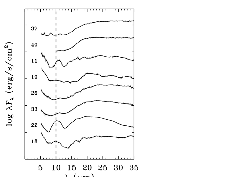
Figure 5: IRS spectra of the non-accreting or non-classified cold disks ordered from bottom to top with growing inner hole radii. The thick and grey lines are the binned and original spectra, respectively and the numbers give their identifications in Table 1.

Some confirmed disks with inner holes show crystalline silicate features, either the forsterite feature at 33 $\mu$m and/or the 23 and 28 $\mu$m complexes (see Olofsson et al. 2009 for definition of these features). The fraction is between 33% and 60% (5-9/15) with the range due to some tentative detections limited by the low signal-to-noise ratio in some spectra. A prominent example of a highly crystalline spectrum is that of object 10, SSTc2d J034227.1+314433, a cold disk in Perseus (see Figure 5). This detection frequency of crystalline material is comparable to the 55% found for the c2d sample of normal CTTS disks based on long-wavelength features, whereas Watson et al. (2009) claim an even higher fraction of 94% for normal disks in Taurus (see discussion in Olofsson et al. 2009).

4.3.2 PAHs

The detection of PAHs is based on at least two of the features at 6.2, 7.7, 8.6, 11.2, 12.8 and 16.4 $\mu$m (Koike et al., 1993; Geers et al., 2006; Tielens, 2008). Overall, PAH features are detected in 13% (2/15) of the cold disks in our sample. This is similar to the fraction of 11–14% found by Geers et al. (2006) for a sample of normal CTTS disks (see also Geers et al. 2007b). This low detection fraction not only reflects the fact that late-type stars have less UV and optical photons to excite the PAHs but also implies a PAH abundance in disks that is typically a factor of 10–100 lower than in the normal interstellar medium, taken to be $5\times 10^{-7}$ with respect to total hydrogen for PAH species with 100 carbon atoms (e.g., C₁₀₀H₂₄) (Geers et al., 2006). Both sources 25 and 27, which have long wavelength fluxes composed of extended material, show exceptionally strong PAH features. Both have low continuum at mid-infrared wavelengths increasing the line-to-continuum contrast. In the case of source 27, even the 16.4 $\mu$m band is clearly revealed (see Fig. 12).

The strong features seen in cold disks do not necessarily imply higher PAH abundances than in normal CTTS disks, however. Dullemond et al. (2007) model the PAH emission in disks with varying degrees of sedimentation, as characterized by the $\alpha$ parameter of turbulence. In the case of low turbulence, $\alpha<10^{-4}$, the big grains quickly sediment to the midplane but the PAHs stay in the upper layers, boosting the feature-to-continuum ratio by a factor of 2–10. For high turbulence, $\alpha\approx 10^{-2}$, the small and big grains stay well mixed in the upper layers, resulting in the typically weak or absent PAHs features consistent with observations (Geers et al., 2006). Dullemond et al. (2007) did not consider disks with inner holes, but qualitatively the effect is similar to their low turbulence case in which the big grains are removed and the features strengths are boosted.

In contrast with the silicates, the PAH emission arises not only from the inner disk but also from the outer disk surface exposed to optical and UV radiation. Indeed, spatially extended PAH emission has been detected out to $\sim$60 AU or more for some disks (Habart et al. 2006, Geers et al. 2007a). Two cold disks within the c2d clouds, SR 21 and T Cha, are included in the observations of Geers et al. (2007b) using VLT-ISAAC and VLT-VISIR to get higher spatial resolution compared with Spitzer. In both cases, the emission is found to be spatially unresolved, with limiting spatial extents (FWHM) of 19 and 13 AU, respectively. These limits are comparable to the values of $R_{\rm Hole}$ of 18 and 15 AU, respectively (Brown et al. 2007, Table A Spitzer c2d Legacy Survey to Identify and Characterize Disks with Inner Dust Holes), indicating that the PAHs are located primarily inside the gaps. For the case of SR 21, the location of the gas inside the gap has been pinpointed to a ring at $\sim 7$ AU radius (Pontoppidan et al., 2008), proving that the gas emission is indeed coming from inside the gap and not from the outer edge or wall of the gap. Since PAHs are likely coupled to the gas, PAH emission, when present, serves as confirmation of the presence of gas inside the gap. Unfortunately we see no correlation between PAHs and accretion, both of which should trace gas within the holes. This is likely due to the dependence of PAH emission on strong UV flux which is lacking from late-type stars.

4.4 Notes on individual sources

Sources 10, 12, 14, 20, 22, 23, 29 and 30 have neither 70 µm  nor 1.3 mm fluxes available. This makes it very difficult to distinguish between a low mass disk and a more massive disk with an inner hole. The difference between the two lies in the presence of a substantial outer disk. The 70µm  limits sometimes hint at the absence of such an outer disk but the limits are not always very stringent. Unless there is compelling evidence from the long wavelength IRS spectra, we have taken the conservative view that these are likely low mass disks and can be explained without needing to invoke an inner hole.

Two sources, 25 and 27, have extremely strong, extended 70 µm  emission and do not appear to be disks. In both cases, it is likely that surrounding material has contaminated the long wavelength photometry, producing these strange SEDs (see Figure 6). Source 25, DoAr 21, has been better studied than many of the other sources in this sample. Resolved imaging of H₂ shows an extended ring structure at 73-219 AU away from the star (Hogeheijde et al. 2009, submitted). Jensen et al. (2009) have speculated that much of the flux in long wavelength unresolved photometry comes from cloud material that the star is heating. Thus, while the SED looks compatible with a large inner hole, this might be due to excess material not directly associated with the star with long wavelength fluxes being increasingly affected. Source 27 has a similar SED and we suspect may arise from a similar physical situation. Both objects show exceptionally strong PAH emission (see Figure 12 and § 4.3.2). Within a disk structure, the strong 70µm  fluxes indicate large amounts of dust at 100-200 AU and good SED fits required unphysical input parameters. Objects with very pronounced 70 $\mu$m excesses but small 24 $\mu$m excesses have been found to be produced by background contamination in the great majority of the cases (Wahhaj et al. 2009, submitted). For these reasons, we have removed these objects from further study.

The 70 µm  flux of source 17 is affected by strong variable background emission, clearly visible in the c2d MIPS-70 image. Two photometric points are given in the SED (Figure 7) with the larger being the full aperture flux and the smaller a PSF aperture flux. The actual flux may be even smaller. The 24 µm  image does not show background emission and is in good agreement with IRS spectra. Although there is evidence for background contamination in the long wavelength SED of this object, a sensible fit was possible with a disk with a hole.

Sources 11, 12, 13, 17, and 18 have stellar temperatures lower than the Kurucz model grid and a blackbody is used instead.

Sources 18, 19 and 24 form a distinct subset of our sample. These three disks all have little to no near-IR excess but very flat disks longward of 8 µm. While there does appear to be a discontinuity between the inner and outer disks, the difference is not large. Despite the unknown disk mass, some degree of settling in the outer disk was required to reproduce the SED shape.

Finally, it is worth noticing that objects 2, 13 and 33 (15% of the cold disk sample) show factor of 2 differences between IRAC and IRS fluxes in the overlapping wavelength range which are too large to be due to calibration errors. In the particular case of object 33, which has the largest difference, only the IRS spectrum hints at a possible inner hole, while the IRAC photometry could be easily explained without a hole. A careful check of the extraction of the IRS spectra and IRAC photometry found no evidence of extended emission, mis-alignment in the IRS observations, or any other instrumental reason for the discrepancy. Indeed, only 6 objects (4%) out of the 147 IRS observed disks in the Serpens IRS survey have similar flux discrepancies between IRAC and IRS (Oliveira, I., 2010, priv. comm.). The IRAC observations were taken approximately 2 years before the spectroscopic ones (see Table 1). Similar scale variability was reported in Muzerolle et al. (2009) for another transitional disk. Such intrinsic variability might be the cause of this phenomenon but systematics between spectra and photometry could cause complications and further investigation is outside the scope of this work.

5 Discussion

5.1 Robust Selection Criteria

5.1.1 Spectroscopic selection criteria for cold disks

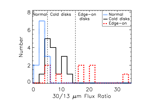
Figure 14: Histogram of F₃₀/F₁₃ ratios for the disks in this paper, with the definition of the boundaries by Brown et al. (2007) marked by vertical dashed lines for comparison. The region on the left is supposed to contain disks without holes, the middle region holds cold disks and on the right edge-on disks. The actual distribution of these types of sources in our sample is shown with normal disks in the blue short dashed line, cold disks with solid black and edge-on disks with the red long dashed line. There is significant overlap between all categories around F₃₀/F₁₃ of 5 but the general trends hold true in our sample.

Determining concrete selection criteria for cold disks is necessary to identify cold disks efficiently out of large Spitzer samples. Previously cold disks have been identified in spectral samples using 30/13 µm  flux ratios and slopes (e.g. Brown et al. 2007; Furlan et al. 2009). These two wavelengths bracket the rise in flux between an inner dust hole and substantial outer disk for holes with radii between 1 and 100 AU around stars with a representative range of stellar masses. The disks in this sample provide confirmation of this classification with 93% (14/15) of the cold disks having $F_{30}$/$F_{13}$ flux ratios between 5 and 15 (see Figure 14). The only disk with $F_{30}$/$F_{13}$$<$5 is Source 2, which has one of the smallest holes. Edge-on disks generally lie above $F_{30}$/$F_{13}$=15 but three overlap with the cold disk region. There is also not a clean separation between normal and cold disks at $F_{30}$/$F_{13}$=5. The 30/13 µm  flux ratio has a crude correlation with larger hole sizes having larger flux ratios, but there is unfortunately no clear relation between the 30/13 µm  flux ratios and the slope between Spitzer 8 and 24 µm  photometry, particularly for cold disks. Thus 8 to 24 µm  slopes and colors cannot be used as a proxy for estimating hole size, although they can be used to select cold disks, as we discuss in the next section.

5.1.2 Photometric selection criteria

To identify the cold disk candidates out of the YSO population, we tested several combinations of color-color diagrams with different Spitzer bands to determine the cleanest identification of disks with inner holes (cold disks). We included not only the results of the detailed SED fitting from § 4.2 but also literature information about cold disks in the c2d clouds including two sources from Brown et al. (2007) and two sources from Andrews et al. (2009). The selection criteria proposed here can be applied to any Spitzer IRAC and MIPS YSO photometric sample of any star-forming region to identify the disks with inner holes.

The criteria are based on colors without dereddening as the extinction to many of the sources in the catalog is unknown. The effects of A_V=10 are plotted as an arrow on the diagrams. The effects are small for extinctions less than 10. Analysis of the spectral sample based on deredden colors provides little difference to the selection regions.

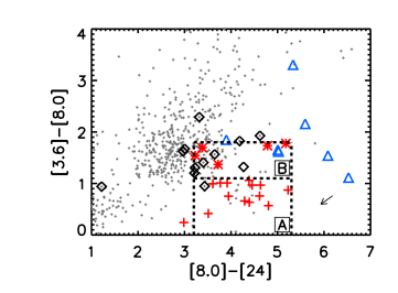
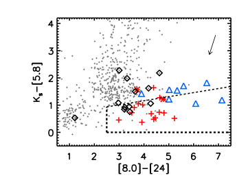
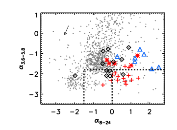
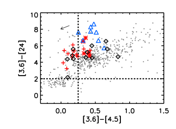
Figure 15: Selection criteria. Red stars and crosses are the spectroscopically confirmed cold disks, black diamonds are disks without holes and blue triangles are edge-on disks. The grey crosses are all the sources in c2d YSO catalog (Evans et al., 2009). (top left) Our selection criteria. Regions A and B define the two selection criteria for identifying cold disks in photometric sample, the first one, represented with red crosses, selects ”clean” inner holes and the second one, represented with red stars, identifies cold disks with near-IR excess. (top right) Selection criteria from Fang et al. (2009). (bottom left) Selection criteria from Muzerolle et al. (2010). (bottom right) Selection criteria from Cieza et al. (2010) with transitional disks according to their definitions in the upper left quadrant. Arrows show the effect of correcting for an extinction of A_V=10.

The cold disk candidate sample is defined with the following cuts in magnitudes, organized in two sections for two different types of objects (see top left Figure 15): Region A selects “clean” inner holes (i.e. disks for which there is no substantial excess in any IRAC band and the signature of an inner opacity hole). Region B selects disks with some excess disk flux in the IRAC bands. The definition of the boundaries are the following:

$${\rm Region\,A:}\,\,0.0\,<\,[3.6]-[8.0]\,<\,1.1\,;\,\,\,3.2\,<\,[8.0]-[24]\,<\,5.3$$ (2)

$${\rm Region\,B:}\,\,1.1\,<\,[3.6]-[8.0]\,<\,1.8\,;\,\,\,3.2\,<\,[8.0]-[24]\,<\,5.3$$ (3)

Region B contains the 4 literature sources plus source 2, while the majority of the new cold disks (13/15) lie in Region A. One possible explanation for this division is the focus of this work on looking for photospheric fluxes in the near-IR, while disks with large holes often have small near-IR excesses (e.g. Brown et al. 2007, Espaillat et al. 2007).

From the overall photometric catalog, the statistics on cold disks within the five c2d clouds can be determined, including sources not included in the spectroscopic follow-up for a variety of reasons such as low fluxes. These disks are marked with small crosses in Figure 15. There are 43 cold disk candidates in Region A accounting for 4% of the total disk population in the c2d YSO catalog. Only one of the objects in that region for which we performed detailed SED modeling including the IRS spectrum was a false positive. This is object 25, DoAr 21, which has a cold disk-like SED but the 70 µm  flux may be strongly contaminated by cloud material (see § 4.4 for further details). From the spectroscopically studied objects in Region A, 93% are cold disks.

Region B is more complicated. While there are well studied, confirmed cold disks within this region, there are many objects which are not cold disks. Region B contains 181 YSOs in the c2d catalog, but fewer sources were selected for our study from this region. Of this small subsample and excluding the rising sources, for which it is not possible to determine the presence of an inner hole in the disk, only 42% of the studied disks turned out to be cold disks, so we estimate a contamination on the order of 58% in this region. These percentages have considerable uncertainty given the low-number statistics. Region B includes the disks WSB 60 and DoAr 44, for which inner holes of 20 and 33 AU, respectively, have been resolved with the SMA but whose SEDs show no detectable signature of them (Andrews et al., 2009). This implies that selecting purely on broadband colors will always be prone to uncertainty. Individual source modeling, spectroscopic studies and non-SED based searches are all needed to fully understand cold disk frequencies, particularly in this region of the color-color parameter space.

If we add together the 43 objects in region A with 42% of the 181 objects in region B, we have a total of 119 cold disks in the sample (12% of the YSO catalog of 1024 sources). Therefore, the fraction of 4% of cold disks quoted above should be interpreted as safe lower limits to the actual population of disks with inner holes in the c2d YSO catalog. The analysis of this photometric sample is outside the scope of this paper and will be presented in a separate article. Considering the IRS flux-limited sample in Serpens where all disks have IRS spectra, we confirm the presence of 8 cold disks, which account for 9% of the total (Oliveira et al., 2010). This range of cold disk frequencies of 4-10% comes with some caveats. Transitional disks with very low mass outer disks are not included in this study (as the ones discussed in e.g. Najita et al. 2007; Cieza et al. 2007), but are often included in other transitional disk frequency statistics. Such disks may represent a later stage of cold disk evolution or a completely different evolutionary pathway. Disks with holes smaller than 1 AU cannot be reliably identified. Disks with large holes but with some near-IR excess can also be difficult to identify from photometry.

A final consideration is the potential bias introduced by the c2d YSO selection criteria themselves. The c2d YSO sample is biased against objects with photospheric colors and only includes sources with good detections at all IRAC bands plus at MIPS 24 $\mu$m band. This obviously imposes bias which is a difficult to determine against selecting transitional disks in regions with very high background emission, like e.g. the IC 348 or $\rho$ Oph clusters. In any case, the effect seems not to be a dominant one since most of the cold disk candidates found with the color selection proposed here are clustered in a similar manner as the rest of the YSOs around the dense high-background clusters, while we should see a lack of such objects in high background areas otherwise.

5.1.3 Comparison with transitional disk selection criteria from other papers

Fang et al. (2009) also recently proposed color-color diagram cuts to select cold disks. Their criteria form a trapezoid in K-[5.8] vs. [8.0]-[24] color-color space defined by K-[5.8] $>$ 0, [8.0]-[24] $>$ 2.5 and the last side by K-[5.8]$<$(0.56+([8.0]-[24])x0.15). In Figure 15b, we evaluate these criteria based on our spectrally confirmed cold disks. Most of the disks in our sample fall within or close to this area. Of our cold disks, 13/15 are within the boundaries while the remaining two are only just above the upper sloped line. However, half (6/12) of the disks without holes also lie within this region as well as some (3/8) of the edge-on disks. Cold disks can be preferentially selected by cutting higher in [8.0]-[24] at $\sim$ 3.5 instead of 2.5. This would exclude more of the candidates that do not have inner holes while including all the disks with holes and also have the benefit of having a greater separation from the bulk sample in the larger catalog (shown in the figure as small gray crosses). The region of [8.0]-[24] between 2.5 and 3.5 has the potential to include transitional disks with low mass outer regions, but individual disk modeling is needed to confirm the nature of these sources. An upper limit in [8.0]-[24] is also needed to remove the edge-on disks, with [8.0]-[24]$<$5 producing a reasonably clean separation.

Muzerolle et al. (2010) use slopes in log $\lambda F_{\lambda}$ vs. log $\lambda$ between 3.6 µm  and 5.8 µm, $\alpha_{3-5}$, vs 8 µm  to 24µm , $\alpha_{8-24}$ . They propose that all transitional disks lie below -1.8 in $\alpha_{3-5}$ with weak excess sources between $\alpha_{8-24}=-1.5$ and $\alpha_{8-24}=0$ and normal cold disks at $\alpha_{8-24}>$0. Our sources lying within the weak excess region were all found not to need holes to fit the SEDs. The normal cold disk region selects similar sources to Region A but sources within Region B are not selected by the Muzerolle et al. (2010) criteria.

Cieza et al. (2010) adopt a wider definition of transitional disks (e.g. they include objects with very small 24 µm excesses), and their selection criteria are therefore less useful for identifying cold disks. Transitional disks are taken to be in the quadrant defined by [3.6]-[24]$>$2 and [3.6]-[4.5]$<$0.25. Just over half (12/19) of the cold disks lie within the selected quadrant, with 7 cold disks missed by this criteria (generally those with more massive outer disks). Almost half (5/12) of the disks without holes lie within the region and in the exact same position as the disks with holes. These disks may be homologously depleted transitional disks. A fairly large fraction of the catalog classical disk locus lies within the selected region and might lead to a large false detection rate of cold disks.

5.2 Properties of the cold disks

One of the most obvious characteristics of this cold disk sample is the relatively small hole sizes (see distribution in Figure 11). Many of the IRS selected cold disks in the literature (e.g. Calvet et al. 2005; Brown et al. 2007; Espaillat et al. 2007; Kim et al. 2009) have large holes with radii greater than 10 AU. Of the 15 cold disks examined here, only three have hole sizes larger than 10 AU while an additional four large hole sources within the clouds are identified in the literature (Brown et al., 2007; Andrews et al., 2009). This may indicate that cold disks with very large holes ($>$10 AU) are intrinsically rarer than disks with smaller holes. Large hole sizes are easy to see from IRS spectra but may not be as obvious from photometry. One complication is that disks with large inner holes often have some near-IR excess making the disks difficult to identify from IRAC colors. Another possible complication arises from the different disk models and methods used to determine the inner disk hole radii. In particular, the possibility cannot be ruled out that the RADMC models, which do not include viscous heating due to accretion tend to produce smaller inner holes than other accreting disk models used by e.g. Calvet et al. (2002). On the other hand, the hole radii determined with same models and methods by Brown et al. (2007) were confirmed by the direct SMA observations of three disks by Brown et al. (2009). Finally, the similarity in terms of infrared SEDs of the two millimeter-discovered cold disks in Ophiuchus (Andrews et al., 2009) to classical disks means millimeter surveys, as well as infrared, would be needed to ensure that all cold disks were found and to robustly confirm this trend. The differences in the definition of transitional disks between the works of Najita et al. (2007) and Cieza et al. (2008a) were also extensively discussed in Cieza et al. (2010).

We find a statistically significant positive correlation between disk mass and hole size (see Figure 16). The correlation has a Pearson’s correlation coefficient of 0.6 and is statistically significant on the 99% level including upper limits on disk mass and on the 90% level with only detected sources. To minimize systematic differences, disk masses for sources from Kim et al. (2009) have been recalculated using the 1.3 mm fluxes in Andrews & Williams (2005) and the flux to disk mass conversion in Section 4.1. The dependence of hole size on disk mass may point to a gravitational process, with more massive disks more likely to form more massive planets in larger orbits. The masses of transitional disks relative to normal disks remains unclear. Najita et al. (2007) finds that transitional disks have larger disk masses for a sample of transitional disks in Taurus, although their disk classification method is different. Cieza et al. (2008b) find very small disk masses for a sample of non-accreting Weak-Lined T Tauri stars. This trend may help explain the different results of the studies as Najita et al. (2007) focused mainly on cold disks from the literature which generally have large holes and are often accreting, while Cieza et al. (2008b) were likely more sensitive to disks with smaller holes and no accretion.

Kim et al. (2009) find a correlation between hole size and stellar mass in their transitional disk sample in Chamaeleon and Taurus. Unfortunately, our sample is too similar in stellar mass to accurately test this trend and there is no correlation found from our sample alone. However, combining with the Kim et al. (2009) sample (see Figure 17) retains a correlation between the size of the inner holes and the stellar masses. The disks from Brown et al. (2007) are in agreement with the Kim et al. (2009) trend while the disks in this paper generally lie below the trend line, indicating smaller hole sizes. This may be partly due to the generally lower disk masses in this sample leading to smaller hole sizes based on the correlation in Figure 16.

Perhaps surprisingly, we see no trends with $L_{\rm Disk}/L_{*}$, a measure of overall disk evolution (see Table A Spitzer c2d Legacy Survey to Identify and Characterize Disks with Inner Dust Holes). $L_{\rm Disk}/L_{*}$ measures the integrated infrared excess normalized by the stellar luminosity and primarily traces the total grain surface area that is reprocessing stellar light. As disks become more tenuous, settle and disappear, the strength of the disk luminosity should decline. This measure is commonly used in debris disk studies (e.g. Morales et al. 2009). There is no correlation with hole size nor are there significant differences in $L_{\rm Disk}/L_{*}$ between the sources with and without holes in this sample. Therefore, if $L_{\rm Disk}/L_{*}$ can indeed be used as a probe for disk flaring, then this points to a distinct lack of settling in the outer regions of cold disks. Alternatively, this might also imply that $L_{\rm Disk}/L_{*}$ is not especially sensitive to the changes in the disk flaring while the outer disk keeps being optically thick.

The majority (9/12, 75%) of the cold disks with H$\alpha$ spectra are accreting. Accretion is a particularly interesting diagnostic in transitional disks as it indicates material inside the hole. Large fractions of accreting cold disks indicate that in many cases gas must be flowing through the hole as any inner gas reservoir would drain quickly. This is in contrast with the results by Najita et al. (2007), who report lower mass accretion rates in transitional disks with respect to the classical T Tauri stars in Taurus, although using a completely different definition of transitional disk from the one used here.

Silicate emission probes dust properties such as grain size and crystallinity. Silicate emission, especially the distinct 10 µm  silicate stretching band, is seen from all but one of the cold disks. However, the presence and intensity of the 10 $\mu$m feature decreases substantially for inner holes radii larger than 7-10 AU (Figure 18). This is partly to be expected as dust-depleted inner holes result in a lack of silicate grains at the correct disk temperatures to produce the features. A large fraction of the cold disks show crystalline features at wavelengths longer than 20 µm  indicating processing which likely occurred in the inner regions of the disks where temperature and densities are high. These regions are now largely depleted in the cold disks but dust mixing, fragmentation of larger bodies or alternative formation routes have resulted in detectable amounts remaining further out in the disk.

5.3 The possible origins of the inner holes

The origins of inner holes are still under debate among several theories developed to explain inner holes and gaps in protoplanetary disks, including i) EUV photoevaporation of the inner disk (Clarke et al., 2001; Alexander et al., 2006), ii) settling and coagulation of dust into large particles (Tanaka et al., 2005; Dullemond & Dominik, 2005), or iii) by the dynamical perturbation of unresolved companions, both stars (Artymowicz & Lubow, 1994) and planets (Quillen et al. 2004; Varnière et al. 2006). It is likely that all are present on some level but it is not clear which are dominant in which systems Cieza et al. (2010); Sicilia-Aguilar et al. (2010).

For photoevaporation, an inner hole occurs when the photoevaporation rate driven by the EUV ionizing flux from the central star matches the viscous accretion rate (Alexander et al., 2006). FUV photoevaporation also plays a significant role in dissipating disks but predominantly removes less bound gas from the outer regions and would therefore not create cold disk SEDs (Gorti & Hollenbach, 2009). Photoevaporation is most effective when accretion rates are low and would result in no gas or dust close to the star within 0.1-1 Myr, depending on assumed disk properties such as viscosity and treatment of the UV ionizing flux (Alexander et al. 2006; Gorti & Hollenbach 2009). The presence of accretion in such a large fraction (75%) of this sample discards photoevaporation as the primary origin. Some disks with inner holes do show evidence for photoevaporation based on [Ne II] observations but the implied mass loss rates are too low to disperse the disk in under 10 Myr (Pascucci & Sterzik, 2009). The disk masses of the remaining 25% are typically low enough that photoevaporation could be the cause of the inner hole.

Accelerated grain growth in the inner regions could produce cold disk SEDs as dust grains became too big to be observed (Tanaka et al., 2005). Models predict that dust particles grow and settle towards the dense disk mid-plane, where they may stick together to form planetesimals (Weidenschilling, 2000). Growth is likely preferential in the inner disk, and these larger bodies will grow and can eventually accrete a large fraction of the surrounding gas to become giant planets (Bryden et al. 1999; Wuchterl et al. 2000 and references therein). In this scenario, grain growth and settling would happen throughout the disk but with faster timescales in the inner region. If grain growth is accompanied by settling throughout the disk, decreasing $L_{\rm Disk}/L_{*}$ with increasing hole size would be expected. We do not see this for our sample making this unlikely to be the dominant scenario although such a correlation for a subsample of the sources may be masked by short inner disk settling timescales or objects formed by different mechanisms. Another potential complication is that coagulation in the inner regions would not effect $L_{\rm Disk}/L_{*}$ in the absence of settling in the outer disk. Holes created via grain growth are likely to have more gradual hole edges compared to holes created by companions.

Binary companions are a possible explanation for cold disk SEDs. Some candidate cold disks, such as CoKu Tau 4, have been later determined to be circumbinary (Ireland & Kraus, 2008). The issue clearly requires further high-resolution imaging of these sources (e.g. Marois et al. 2008; Kalas et al. 2008; Lagrange et al. 2009) or radial velocity measurements to confirm the possible presence of stellar or substellar-mass companions. However, this is time consuming for large samples and may not even be possible for more distant regions or planets at larger radii which require long term monitoring. Preliminary results of binary searches show that close binary companions often result in the complete dissipation of the disk and that circumbinary “transition” disks may not be common (Kraus et al., 2009; Pott et al., 2010). If stellar companions carve out inner holes, accretion may either continue or cease depending on the separation and mass ratio of the two stars (Artymowicz & Lubow, 1996; Ireland & Kraus, 2008). On the other hand, if a planet carves out an inner hole accretion can continue at a reduced rate aided by mechanisms such as the magneto-rotational instability (Chiang & Murray-Clay, 2007).

Inner holes created by planets remains a popular and exciting explanation. Of the scenarios described this is the most difficult to positively confirm or deny. Planets are faint so direct observation is difficult while their small masses leave weaker gravitational signatures on the disk than stellar companions. The inner hole radii are compatible with the distribution of exoplanet semi-major axis, as found in the latest exoplanet database as of December 2009 (Fig. 17). As the exoplanets likely formed in similar disks before dissipation, it is likely that there are young exo-planets in some disks at these types of radii but whether they are responsible for the cold disk signatures discussed in this paper remains to be determined.

6 Summary

The main results of this work are summarized here:

• Optical spectra, 2MASS and Spitzer photometry, millimeter continuum observations and Spitzer/IRS 5 to 35 $\mu$m spectra of a sample of 35 cold disk candidates selected from c2d photometry are presented and analyzed.

• Out of 35 objects in the initial sample, SED modeling identifies 15 as disks with inner holes, which we call “cold disks”, following the c2d convention (Brown et al., 2007). Of the remaining sources, 10 could be modelled without holes, 8 are edge-on disks and 2 have SEDs strongly contaminated by cloud material.

• The color cuts $0.0<[3.6]-[8.0]<1.1$ and $3.2<[8.0]-[24]<5.3$ identify most cold disks from this sample ($\sim$ 80%), in particular those with the cleanest inner holes. Extension of the $[3.6]-[8.0]$ color cut to 1.8 recovers some objects with small near-IR excesses and large holes, but contains contamination from disks without holes. Out of the large c2d YSO sample, between $\sim$ 12% of the disks are estimated to be cold disks based on these selection criteria.

• We evaluated the criteria of Fang et al. (2009), Muzerolle et al. (2010) and Cieza et al. (2010) and suggest improvements based on our spectroscopic study.

• The cold disks presented here have small hole sizes, generally less than 10 AU. This distribution is more in agreement with exoplanet radii than the large hole sizes of most cold disks in the literature.

• A large fraction (75%) of the cold disks are accreting, suggesting that gas is flowing through the dust depleted hole. This large fraction of accreting disks is not in agreement with the dominant hole origin being photoevaporation.

• Hole size correlates with disk mass with more massive disks tending to have larger holes.

• The sizes of the inner holes scale linearly with the stellar mass although with a large spread.

• The 10 $\mu$m silicate features in the sample show substantial grain growth. The 10 $\mu$m silicate emission feature strength with respect to continuum decreases drastically for inner holes larger than $\sim$ 7 AU. Some (33-60%) of the cold disks show long wavelength crystalline features indicating that mixing from the inner regions where crystallization occurs to outside the inner hole region must be efficient. Only 2 sources ($\sim$ 13%) show PAH emission.

Table 1: Cold disk candidates and Spitzer observing log

					Prog-		IRS		MIPS-70
ID	Name	Cloud	$\alpha_{K-24}$	$\alpha_{8-24}$	ram1	Refs.	AOR	Obs. Date	AOR	Obs. Date
1	SSTc2d J032835.1+302010	Per	0.15	2.13	1	1,15	19059712	2007-03-18	19954688	2007-02-03
2	ASR 118	Per	-0.22	0.77	1	2,15	19056128	2006-09-19	19057664	2007-09-20
3	SSTc2d J032903.9+305630	Per	-0.17	1.25	1	15	19954176	2007-03-19	19954688	2007-02-03
4	SSTc2d J032924.1+311958	Per	0.36	1.57	1	1,15	19052544	2007-03-22	19057664	2007-09-20
5	SSTc2d J032929.3+311835	Per	-0.66	1.30	1	2,15	19053312	2007-03-09	19057664	2007-09-20
6	SSTc2d J033027.2+302830	Per	0.00	2.37	1	1,15	19953920	2007-03-09	19057664	2007-09-20
7	SSTc2d J033035.5+311559	Per	-0.19	2.04	1	15	19053056	2007-03-09	19954688	2007-02-03
8	SSTc2d J033038.2+303212	Per	0.35	2.98	1	15	19953664	2007-03-19	19057664	2007-09-20
9	LZK 21	Per	-0.66	0.06	1	3,15	19052032	2007-03-09	19954688	2007-02-23
10	SSTc2d J034227.1+314433	Per	-0.93	0.74	1	15	19053568	2007-03-18	19954432	2007-09-18
11	Cl* IC 348 LRL 190	Per	-1.00	0.05	1	4,6,7,15	19054848	2007-03-18	19954432	2007-09-18
12	SSTc2d J034434.8+315655	Per	-1.11	0.65	1	4,5,6,15	19053824	2007-03-15	19954432	2007-09-18
13	Cl* IC 348 LRL 265	Per	-0.09	0.33	1	15	19052288	2006-09-18	19954432	2007-09-18
14	Cl* IC 348 LRL 110	Per	-0.60	0.50	1	4,6,7,15	19052288	2006-09-18	19954432	2007-09-18
15	LkH$\alpha$ 329	Per	-1.02	-0.24	1	8,15	19056384	2007-03-09	19954432	2007-09-18
16	Hn 24	Cha	-0.85	-0.16	1	9,16	19054592	2007-03-11	19058944	2006-08-15
17	Sz 84	Lup	-2.34	-0.49	2	10,19	05644288	2004-03-25	5697024	2005-03-07
18	SSTc2d J161029.6-392215	Lup	-1.07	0.01	1	17	19051008	2007-03-19	19055360	2006-08-18
19	RX J1615.3-3255	Oph	-1.64	-0.10	2	11,19	15916800	2005-09-09	5703424	2005-03-07
20	SSTc2d J162148.5-234027	Oph	-0.33	0.32	1	18	15920896	2005-09-09	…	…
21	SSTc2d J162221.1-230403	Oph	0.93	1.43	1	18	15920896	2005-09-09	…	…
22	SSTc2d J162245.4-243124	Oph	-0.83	0.69	1	18	15920641	2006-03-15	…	…
23	SSTc2d J162332.9-225847	Oph	-1.07	-0.37	1	18	15920641	2006-03-15	…	…
24	SSTc2d J162506.9-235050	Oph	-1.10	0.68	1	18	19059200	2007-03-19	19954944	2006-09-01
25	DoAr 21	Oph	-1.16	-0.43	3	12,13,18	12699392	2006-03-15	…	…
26	SSTc2d J182829.1+002756	Ser	-0.67	-0.11	4	20	17885184	2007-04-24	…	…
27	SSTc2d J182858.1+001724	Ser	-1.92	-2.97	4	20	17888768	2007-05-05	…	…
28	SSTc2d J182907.0+003838	Ser	-0.75	-1.48	4	20	17884672	2007-04-28	…	…
29	SSTc2d J182911.5+002039	Ser	-0.85	0.03	4	20	17887744	2007-04-24	…	…
30	SSTc2d J182915.6+003912	Ser	-0.31	-1.21	1	20	17884672	2007-04-28	19057152	2007-05-18
31	SSTc2d J182915.6+003923	Ser	-0.47	-0.73	1	20	17885440	2007-04-24	…	…
32	SSTc2d J182935.6+003504	Ser	-1.02	-0.40	1	20	17884160	2007-04-19	19057152	2007-05-18
33	SSTc2d J182936.2+004217	Ser	-0.68	-0.32	4	20	17884160	2007-04-19	…	…
34	SSTc2d J182944.1+003356	Ser	-1.41	-1.05	4	20	17886720	2007-04-24	…	…
35	SSTc2d J182947.3+003223	Ser	-0.90	-1.50	1	20	17887488	2007-04-25	19057152	2007-05-18

Table 2: IRAC, MIPS and MAMBO 1.3 mm fluxes for the cold disk candidate sample

No.	IRAC $3.6$	IRAC $4.5$	IRAC $5.8$	IRAC $8.0$	MIPS $24.0$	MIPS $70.0$	$1.3$ mm
	(mJy)	(mJy)	(mJy)	(mJy)	(mJy)	(mJy)	(mJy)
1	1.45e+00$\pm$1.52e-02	1.18e+00$\pm$1.52e-02	9.55e-01$\pm$2.08e-02	1.21e+00$\pm$2.19e-02	4.25e+01$\pm$2.44e-01	1.22e+02$\pm$4.69e+00	$<$1.00e+00
2	1.68e+01$\pm$2.74e-01	1.47e+01$\pm$2.74e-01	1.21e+01$\pm$1.02e-01	1.75e+01$\pm$1.20e-01	1.78e+02$\pm$9.73e-01	3.40e+02$\pm$9.35e+01	3.70e+00$\pm$9.00e-01
3	9.64e-01$\pm$7.40e-03	9.87e-01$\pm$7.40e-03	8.28e-01$\pm$1.15e-02	8.94e-01$\pm$1.34e-02	1.14e+01$\pm$1.21e-01	4.00e+01$\pm$4.06e+00	$\ldots$
4	2.01e+00$\pm$3.51e-02	2.00e+00$\pm$3.51e-02	2.05e+00$\pm$3.10e-02	3.28e+00$\pm$3.21e-02	6.78e+01$\pm$4.41e-01	$<$3.75e+01	1.20e+00$\pm$1.30e+00
5	1.28e+01$\pm$2.68e-01	9.33e+00$\pm$2.68e-01	6.96e+00$\pm$6.71e-02	6.19e+00$\pm$4.73e-02	9.55e+01$\pm$6.05e-01	3.06e+02$\pm$1.31e+01	6.30e+00$\pm$1.10e+00
6	1.51e+01$\pm$1.43e-01	1.50e+01$\pm$1.43e-01	1.05e+01$\pm$6.43e-02	8.42e+00$\pm$5.92e-02	4.31e+02$\pm$2.33e+00	1.22e+03$\pm$8.20e+00	$<$7.00e-01
7	1.46e+00$\pm$7.30e-02	1.18e+00$\pm$5.86e-02	1.02e+00$\pm$6.46e-02	1.38e+00$\pm$7.64e-02	4.17e+01$\pm$3.86e+00	1.45e+02$\pm$4.06e+00	1.30e+00$\pm$5.00e-01
8	1.05e+00$\pm$1.54e-02	1.03e+00$\pm$1.54e-02	8.18e-01$\pm$1.96e-02	6.43e-01$\pm$1.81e-02	5.75e+01$\pm$3.29e-01	2.88e+02$\pm$6.25e+00	$\ldots$
9	9.37e+01$\pm$1.11e+00	8.70e+01$\pm$1.11e+00	7.81e+01$\pm$4.61e-01	8.57e+01$\pm$7.27e-01	3.07e+02$\pm$1.84e+00	4.02e+02$\pm$8.60e+00	1.30e+01$\pm$1.30e+00
10	1.32e+01$\pm$1.21e-01	9.87e+00$\pm$1.21e-01	7.23e+00$\pm$5.75e-02	5.50e+00$\pm$4.83e-02	4.68e+01$\pm$2.81e-01	$<$8.39e+01	$<$1.40e+00
11	6.68e+00$\pm$4.26e-02	5.22e+00$\pm$4.26e-02	4.21e+00$\pm$2.74e-02	3.62e+00$\pm$4.19e-02	1.39e+01$\pm$1.62e-01	2.50e+01$\pm$6.60e+01	$\ldots$
12	1.13e+01$\pm$6.18e-02	8.65e+00$\pm$6.18e-02	6.47e+00$\pm$3.54e-02	4.56e+00$\pm$3.94e-02	2.10e+01$\pm$1.53e-01	$<$7.60e+01	$<$1.40e+00
13	1.23e+01$\pm$1.71e-01	1.43e+01$\pm$1.71e-01	1.31e+01$\pm$1.14e-01	1.41e+01$\pm$1.40e-01	1.23e+02$\pm$8.81e-01	$<$1.37e+02	1.16e+01$\pm$1.00e+00
14	1.32e+01$\pm$2.18e-01	1.15e+01$\pm$2.18e-01	8.93e+00$\pm$1.04e-01	1.15e+01$\pm$2.06e-01	6.71e+01$\pm$5.85e-01	$<$2.16e+03	$<$1.46e+00
15	1.27e+02$\pm$1.62e+00	1.02e+02$\pm$1.62e+00	7.66e+01$\pm$4.10e-01	7.07e+01$\pm$5.18e-01	1.75e+02$\pm$8.47e-01	1.31e+02$\pm$7.86e+00	$<$1.20e+00
16	1.16e+02$\pm$6.70e+00	8.65e+01$\pm$4.69e+00	7.71e+01$\pm$3.99e+00	9.68e+01$\pm$4.78e+00	2.48e+02$\pm$2.30e+01	3.18e+02$\pm$3.37e+00	$\ldots$
17	4.20e+01$\pm$3.51e-02	2.90e+01$\pm$3.51e-02	2.01e+01$\pm$3.10e-02	1.20e+01$\pm$3.21e-02	2.09e+01$\pm$4.41e-01	2.44e+02$\pm$ 7.32e+01	$<$3.60e+01
18	1.91e+01$\pm$9.30e-01	1.42e+01$\pm$9.30e-01	1.15e+01$\pm$5.60e-01	1.09e+01$\pm$5.30e-01	3.37e+01$\pm$3.18e+00	1.10e+02$\pm$1.80e+01	$\ldots$
19	1.14e+02$\pm$9.30e-01	8.50e+01$\pm$9.30e-01	6.10e+01$\pm$5.60e-01	6.60e+01$\pm$5.30e-01	2.71e+02$\pm$3.18e+00	7.27e+02$\pm$1.80e+01	$\ldots$
20	1.24e+01$\pm$6.00e-01	1.20e+01$\pm$5.70e-01	1.08e+01$\pm$5.20e-01	1.52e+01$\pm$7.30e-01	7.99e+01$\pm$7.39e+00	$<$6.82e+01	$<$4.60e+00
21	1.61e+00$\pm$8.00e-02	1.60e+00$\pm$7.00e-02	1.78e+00$\pm$1.00e-01	7.72e+00$\pm$3.80e-01	1.17e+02$\pm$1.08e+01	$<$5.38e+02	$<$4.40e+00
22	9.21e+01$\pm$4.58e+00	6.15e+01$\pm$3.04e+00	4.47e+01$\pm$2.14e+00	5.13e+01$\pm$2.47e+00	3.45e+02$\pm$3.20e+01	$<$8.31e+01	$<$5.40e+00
23	3.23e+01$\pm$1.61e+00	2.44e+01$\pm$1.17e+00	1.92e+01$\pm$9.20e-01	2.23e+01$\pm$1.07e+00	4.79e+01$\pm$4.47e+00	$<$4.32e+02	$\ldots$
24	6.07e+01$\pm$2.74e-01	4.17e+01$\pm$2.74e-01	3.09e+01$\pm$1.02e-01	2.28e+01$\pm$1.20e-01	1.59e+02$\pm$9.73e-01	5.37e+02$\pm$7.88e+01	$\ldots$
25	1.19e+03$\pm$1.94e+01	8.45e+02$\pm$1.49e+01	7.30e+02$\pm$1.00e+01	6.39e+02$\pm$8.50e+00	1.34e+03$\pm$3.42e+01	1.20e+04$\pm$1.26e+03	$\ldots$
26	9.80e+00$\pm$5.75e-01	8.51e+00$\pm$5.75e-01	7.03e+00$\pm$3.82e-01	5.46e+00$\pm$2.98e-01	4.34e+01$\pm$4.03e+00	$<$2.87e+02∗	2.40e+01$\pm$6.00e-01
27	5.25e+01$\pm$2.97e+00	3.67e+01$\pm$2.97e+00	3.12e+01$\pm$1.68e+00	2.85e+01$\pm$1.68e+00	9.74e+00$\pm$9.20e-01	1.17e+03$\pm$1.01e+02	$\ldots$
28	2.13e+01$\pm$1.43e+00	2.93e+01$\pm$1.43e+00	2.25e+01$\pm$1.29e+00	2.27e+01$\pm$1.10e+00	4.02e+01$\pm$3.72e+00	$<$2.87e+02∗	$\ldots$
29	4.46e+00$\pm$2.73e-01	3.36e+00$\pm$2.73e-01	2.39e+00$\pm$1.47e-01	1.72e+00$\pm$1.03e-01	1.60e+01$\pm$1.49e+00	$<$2.87e+02∗	$\ldots$
30	1.36e+01$\pm$8.67e-01	1.62e+01$\pm$8.67e-01	1.51e+01$\pm$8.86e-01	2.56e+01$\pm$1.26e+00	6.05e+01$\pm$5.59e+00	$<$5.00e+01	$\ldots$
31	6.42e+00$\pm$4.61e-01	7.33e+00$\pm$4.61e-01	5.99e+00$\pm$3.46e-01	8.05e+00$\pm$3.94e-01	3.25e+01$\pm$3.01e+00	1.35e+02$\pm$1.57e+01	$\ldots$
32	3.05e+01$\pm$2.00e+00	2.41e+01$\pm$2.00e+00	1.70e+01$\pm$9.68e-01	1.28e+01$\pm$6.61e-01	7.42e+01$\pm$6.86e+00	5.76e+01$\pm$1.31e+01	$\ldots$
33	2.11e+01$\pm$1.24e+00	1.99e+01$\pm$1.24e+00	1.56e+01$\pm$8.31e-01	1.28e+01$\pm$6.19e-01	8.11e+01$\pm$7.49e+00	1.26e+02$\pm$1.74e+01	2.30e+00$\pm$6.00e-01
34	2.08e+01$\pm$1.19e+00	1.37e+01$\pm$1.19e+00	1.10e+01$\pm$5.91e-01	6.97e+00$\pm$3.45e-01	1.97e+01$\pm$1.83e+00	1.40e+02$\pm$1.71e+01	6.30e+00$\pm$6.00e-01
35	1.04e+01$\pm$6.24e-01	9.28e+00$\pm$6.24e-01	8.20e+00$\pm$4.53e-01	1.06e+01$\pm$5.43e-01	1.82e+01$\pm$1.69e+00	1.76e+01$\pm$6.81e+00	2.20e+00$\pm$9.00e-01

References. — 1) Walawender et al. (2005), 2) Getman et al. (2002), 3) Liu et al. (1980), 4) Luhman et al. (1998), 5) Muench et al. (2007), 6) Preibisch et al. (2003), 7) Preibisch & Zinnecker (2001), 8) Herbig & Bell (1988), 9) Hartigan (1993), 10) Schwartz (1977), 11) Krautter et al. (1997), 12) Dolidze & Arakelyan (1959), 13) Gagné et al. (2004), 14) Aspin et al. (1994), 15) Lai et al. (in prep.), 16) Alcalá et al. (2008), 17) Merín et al. (2008), 18) Allers et al. (2006), 19) Padgett et al. (2006), 20) Harvey et al. (2007), 21) Brown et al. (2007), 22) Brown et al. (2008), 23) Kessler-Silacci et al. (2006)

Table 3: Optical spectroscopy observation log

Date	Telescope +	Grism	Wavelength	Dispersion	colheadID
	Instrument		Coverage	(Å/resel)
2006 November 22	WHT+WYFFOS	R600R	5500–8500	4	2, 3, (4), 5, 7, (10), (11)
					12, 13, 14, 15
2006 December 13					1, (9)
2007 July 26	WHT+ISIS	R600R	6000–8000		24
2008 July 22					2
2007 May 06	INT+IDS	R600R	4700–8700		22, 24
2008 June 23-25	2.2m/CAFOS	R100	6000–9000	2	21, 23, 24, 25, 29
2008 December 30	Palomar/DBSP	R316	6200–8700	10	4, 6, 8
2009 July 21	Palomar/DBSP	R316	6200–8700		9, 10
2009 October 30	WHT+ISIS	R316	5500–8300		10, 13
2009 August 03	CTIO 1.5m/R-C Spec	47/Ib	5630–6930		18,19

Table 4: Stellar parameters for the stars in the sample.

No.	Object Id.	SpT	Ref	AV	Teff	L∗	Mass	EW[H$\alpha$]∗	H$\alpha$[10%]	$\log\dot{M_{acc}}$
				(mag)	(K)	(L⊙)		(Å)	(km/s)	(M⊙/yr)
2	ASR 118	K4	1	13.0	4590	1.17	1.36	26	293	-10.2
5	SSTc2d J032929.3+311835	M0	1	…	3850	0.09	…	4.8	…	…
10	SSTc2d J034227.1+314433	K7	1	5.0	4060	0.22	0.82	4.3	…	…
11	Cl* IC 348 LRL 190	M3.75	6	6.5	3306	0.09	0.35	5	…	…
12	SSTc2d J034434.8+315655	M3	1	3.0	3415	0.12	0.45	130	504	-8.0
17	Sz 84	M5.5	3	0.5	3057	0.15	0.14	44	…	…
18	SSTc2d J161029.6-392215	M5	1	1.0	3125	0.08	0.21	18	…	…
19	RX J1615.3-3255	K4	1	1.0	4590	0.85	1.28	26	…	…
22	SSTc2d J162245.4-243124	M2	1	2.0	3580	0.29	0.59	5.0	224	…
24	SSTc2d J162506.9-235050	M0.5	1	3.0	3778	0.21	0.77	4.6	505	-8.0
26	SSTc2d J182829.1+002756	K7	2	13.0	4060	0.34	0.94	…	…	…
29	SSTc2d J182911.5+002039	M0	13	6.0	3850	0.13	0.72	25	656	-6.5
32	SSTc2d J182935.6+003504	K7	13	4.0	4060	0.52	1.06	10.9	273	-10.2
33	SSTc2d J182936.2+004217	F9	13	11.0	6115	1.89	1.30	…	…	…
34	SSTc2d J182944.1+003356	M0	13	5.0	3850	0.54	0.93	37	444	-8.6
1	SSTc2d J032835.1+302010†	K4	1	0.0	4590	0.07∗	…	8.1	449	-8.5
3	SSTc2d J032903.9+305630†	G7	1	6.0	5630	0.05∗	…	54	344	-9.6
4	SSTc2d J032924.1+311958†	K5	1	5.0	4350	0.41	0.96	6.5	262	-10.4
6	SSTc2d J033027.2+302830†,a	cb	1	…	…	…	…	106	…	…
7	SSTc2d J033035.5+311559†	K5	1	…	4350	0.07∗	…	15.1	405	-9.0
8	SSTc2d J033038.2+303212†	M0c	1	…	3850	0.05∗	…	…	194	…
9	LZK 21	M0	1	6.0	3850	1.46	1.00	72	…	…
13	Cl* IC 348 LRL 265	M3	1	17.	3415	0.42	0.52	113	…	…
14	Cl* IC 348 LRL 110	M0.5	1	5.0	3778	0.22	0.78	36	424	-8.8
15	LkH$\alpha$ 329	K5	1	5.0	4350	2.89	1.63	19.4	700	-6.1
16	Hn 24	M0.5	1	2.0	3778	0.75	0.92	0.2	311	…
20	SSTc2d J162148.5-234027	M5.5	5	7.0	3057	0.04	0.14	…d	…	…
21	SSTc2d J162221.1-230403†	K5	1	…	4350	0.02∗	…	45.8	594	-7.1
23	SSTc2d J162332.9-225847	M0.5	1	5.0	3778	0.15	0.73	2.8	413	…
25	DoAr 21	K1	4	6.0	5080	9.84	1.80	1–2	450	…
27	SSTc2d J182858.1+001724	G3	13	6.0	5830	4.76	1.4	-2.2	…	…
28	SSTc2d J182907.0+003838	K7	2	16.0	4060	0.6	1.04	…	…	…
30	SSTc2d J182915.6+003912	K5	13	12.0	4350	0.45	1.00	22	532	-7.7
31	SSTc2d J182915.6+003923†	K7	2	0.0	4060	0.20	…	…	…	…
35	SSTc2d J182947.3+003223	M0	13	7.0	3850	0.28	0.85	49	618	-6.9

Note. — For clarity, cold disks are shown above the horizontal line while other objects are below.

Note. — We used the c2d distances to the clouds to compute the stellar luminosities: 250 pc for Perseus, 187 pc for Cham. II, 150 pc for Lupus II and III, 120 pc for Ophiuchus and 260 pc for Serpens.

References. — 1) Spectral type from this work with optical spectroscopy; 2) Spectral type from this work with photometry; 3) Krautter et al. (1997); 4) Jensen et al. (2009) 5) Gully-Santiago et al. in prep. 6) Luhman et al. (2003) 13) Oliveira et al. (2009)

Table 5: Optical and near-IR photometry for the cold disk candidate sample

No.	$U$	$B$	$V$	$R_{C}$	$I_{C}$	$J_{2MASS}$	$H_{2MASS}$	$K_{2MASS}$
	(mag)	(mag)	(mag)	(mag)	(mag)	(mag)	(mag)	(mag)
1	$\ldots$	$\ldots$	$\ldots$	$\ldots$	$\ldots$	15.66$\pm$0.05	14.41$\pm$0.05	13.69$\pm$0.05
2	$\ldots$	$\ldots$	$\ldots$	$\ldots$	$\ldots$	13.76$\pm$0.05	11.92$\pm$0.05	11.08$\pm$0.05
3	$\ldots$	$\ldots$	$\ldots$	$\ldots$	$\ldots$	15.64$\pm$0.05	14.64$\pm$0.05	14.37$\pm$0.05
4	$\ldots$	$\ldots$	$\ldots$	$\ldots$	$\ldots$	15.52$\pm$0.05	14.25$\pm$0.05	13.57$\pm$0.05
5	$\ldots$	$\ldots$	$\ldots$	$\ldots$	$\ldots$	12.59$\pm$0.05	11.37$\pm$0.05	10.96$\pm$0.05
6	$\ldots$	$\ldots$	$\ldots$	$\ldots$	$\ldots$	14.86$\pm$0.05	13.16$\pm$0.05	11.90$\pm$0.05
7	$\ldots$	$\ldots$	$\ldots$	$\ldots$	$\ldots$	15.66$\pm$0.09	14.40$\pm$0.06	13.69$\pm$0.05
8	$\ldots$	$\ldots$	$\ldots$	$\ldots$	$\ldots$	15.57$\pm$0.05	14.65$\pm$0.05	14.04$\pm$0.05
9	$\ldots$	$\ldots$	$\ldots$	$\ldots$	$\ldots$	11.29$\pm$0.05	10.05$\pm$0.05	9.41$\pm$0.05
10	$\ldots$	$\ldots$	$\ldots$	$\ldots$	16.33$\pm$0.01	13.38$\pm$0.05	11.86$\pm$0.05	11.15$\pm$0.05
11	$\ldots$	$\ldots$	$\ldots$	20.45$\pm$0.05	17.93$\pm$0.05	14.38$\pm$0.05	12.87$\pm$0.05	12.11$\pm$0.05
12	$\ldots$	$\ldots$	$\ldots$	$\ldots$	$\ldots$	13.02$\pm$0.05	12.09$\pm$0.05	11.63$\pm$0.05
13	$\ldots$	$\ldots$	$\ldots$	$\ldots$	$\ldots$	15.64$\pm$0.05	13.37$\pm$0.05	12.00$\pm$0.05
14	$\ldots$	$\ldots$	$\ldots$	$\ldots$	15.78$\pm$0.05	13.07$\pm$0.05	11.85$\pm$0.05	11.28$\pm$0.05
15	$\ldots$	$\ldots$	$\ldots$	$\ldots$	$\ldots$	10.46$\pm$0.05	9.46$\pm$0.05	8.93$\pm$0.05
16	$\ldots$	$\ldots$	$\ldots$	$\ldots$	$\ldots$	10.15$\pm$0.05	9.33$\pm$0.05	8.88$\pm$0.05
17	$\ldots$	17.54$\pm$0.03	16.06$\pm$0.11	14.53$\pm$0.04	12.94$\pm$0.02	10.93$\pm$0.02	10.20$\pm$0.02	9.85$\pm$0.02
18	$\ldots$	17.51$\pm$0.03	16.31$\pm$0.01	15.79$\pm$0.05	13.90$\pm$0.05	11.94$\pm$0.05	11.27$\pm$0.05	10.91$\pm$0.05
19	$\ldots$	$\ldots$	12.04$\pm$0.01	11.28$\pm$0.05	10.54$\pm$0.05	9.55$\pm$0.05	8.78$\pm$0.05	8.56$\pm$0.05
20	$\ldots$	$\ldots$	$\ldots$	19.59$\pm$0.04	$\ldots$	13.59$\pm$0.05	12.35$\pm$0.05	11.69$\pm$0.05
21	$\ldots$	19.18$\pm$0.03	17.74$\pm$0.01	17.03$\pm$0.04	$\ldots$	14.66$\pm$0.05	13.87$\pm$0.05	13.57$\pm$0.05
22	$\ldots$	$\ldots$	15.74$\pm$0.50	14.82$\pm$0.05	12.51$\pm$0.02	10.37$\pm$0.05	9.43$\pm$0.05	9.06$\pm$0.05
23	$\ldots$	$\ldots$	$\ldots$	16.22$\pm$0.04	$\ldots$	11.49$\pm$0.05	10.68$\pm$0.05	10.29$\pm$0.05
24	$\ldots$	18.38$\pm$0.05	16.59$\pm$0.05	15.55$\pm$0.05	$\ldots$	11.06$\pm$0.05	10.03$\pm$0.05	9.51$\pm$0.05
25	$\ldots$	15.80$\pm$0.75	14.00$\pm$0.50	12.00$\pm$0.05	10.05$\pm$0.90	8.09$\pm$0.02	6.86$\pm$0.05	6.23$\pm$0.02
26	$\ldots$	$\ldots$	$\ldots$	$\ldots$	$\ldots$	14.99$\pm$0.05	12.76$\pm$0.05	11.81$\pm$0.05
27	$\ldots$	$\ldots$	$\ldots$	$\ldots$	$\ldots$	10.72$\pm$0.05	9.83$\pm$0.05	9.45$\pm$0.05
28	$\ldots$	$\ldots$	$\ldots$	$\ldots$	$\ldots$	15.20$\pm$0.05	12.90$\pm$0.05	11.55$\pm$0.05
29	$\ldots$	$\ldots$	$\ldots$	$\ldots$	$\ldots$	14.03$\pm$0.05	12.89$\pm$0.05	12.42$\pm$0.05
30	$\ldots$	$\ldots$	$\ldots$	$\ldots$	$\ldots$	14.53$\pm$0.05	12.65$\pm$0.05	11.69$\pm$0.05
31	$\ldots$	$\ldots$	$\ldots$	18.38$\pm$0.05	$\ldots$	14.14$\pm$0.05	12.79$\pm$0.05	12.13$\pm$0.05
32	$\ldots$	$\ldots$	$\ldots$	$\ldots$	$\ldots$	12.00$\pm$0.05	10.84$\pm$0.05	10.26$\pm$0.05
33	$\ldots$	$\ldots$	$\ldots$	$\ldots$	$\ldots$	13.27$\pm$0.05	11.92$\pm$0.05	11.31$\pm$0.05
34	$\ldots$	$\ldots$	$\ldots$	19.04$\pm$0.50	$\ldots$	12.19$\pm$0.05	11.15$\pm$0.05	10.77$\pm$0.05
35	$\ldots$	$\ldots$	$\ldots$	19.14$\pm$0.05	$\ldots$	13.45$\pm$0.05	12.11$\pm$0.05	11.45$\pm$0.05

References. — Optical fluxes come from 1) Bouy et al. (in prep) for Perseus sources (1-15); 2) Spezzi et al. (2008) for the only object from Chamaeleon II (#16); 3) Comerón et al. (2009) for the Lupus sources (# 17 and 18); 4) Bouy et al. (in prep.) for Ophiuchus sources (19 - 25); and 5) Spezzi et al. (2010) for the sources in Serpens (26-35)

Table 6: Selection criteria for edge-on disks

No.	Under	Forbidden	Silicate	Ice	High
	luminous	lines	absorption	absorption	LDisk/L∗
1	✓				✓
3	✓	✓?	✓	✓
4			✓	✓
6		✓			✓
7	✓		✓		✓
8	✓	✓	✓		✓
21	✓	✓			✓
31					✓?

Table 7: Disk physical parameters and observables

No.	Reg.	Rhole∗	Inc.	Mass†	Sett.	Fmm	Mdisk	Ref.	F30/F13	Ldisk/L∗	R${}_{\rm hole}^{\rm Rob.}$	Model ID
		(AU)	(deg)	10-3 M⊙		(mJy)	10-3 M⊙				(AU)	(Rob.)
1	$\ldots$	edge	…	…	…	$<$1.0	$<$0.3	1	20.17	…	…	…
2	B	1.5$\pm$1	75	obs	0.5	3.7$\pm$0.9	1.1$\pm$0.3	1	4.29	0.16	1.64	3005228
3	B	edge	…	…	…	…	…	…	21.35	…	…	…
4	$\ldots$	edge	…	…	…	$<$1.3	$<$0.4	1	9.82	…	…	…
5	A	6${}^{\rm+4}_{\rm-2}$	10	obs	0.5	6.3$\pm$1.1	1.9$\pm$0.3	1	12.86	0.2	15.3	3000829
6	$\ldots$	edge	…	…	…	$<$0.7	$<$0.2	1	17.63	…	…	…
7	B	edge	…	…	…	1.3$\pm$0.5	0.4$\pm$0.2	1	17.47	…	…	…
8	$\ldots$	edge	…	…	…	…	…	…	33.19	…	…	…
9	B	no hole	30	obs	0.5	13.0$\pm$1.3	4.0$\pm$0.4	1	3.01	0.19	…	…
10	A	5$\pm$1	60	0.001	1	$<$1.4	$<$0.4	1	4.76	0.04	1.87	3018041
11	A	5$\pm$1	30	0.003	1	…	…	…	7.85	0.22	0.75	3015642
13	$\ldots$	no hole	45	obs	1	11.6$\pm$1.0	3.5$\pm$0.3	1	4.51	0.18	1.71	3007226
12	A	3$\pm$1	5	0.002	1	$<$1.4	$<$0.4	1	5.9	0.2	1.04	3017747
14	B	no hole	60	0.3	1	$<$1.5	$<$0.5	1	5.78	0.23	0.8	3019220
15	B	no hole	75	0.005	1	$<$1.2	$<$0.4	1	2.38	0.05	8.6	3005263
16	B	no hole	65	0.05	1	…	…	…	2.65	0.12	$\ldots$	3012969
17	$\ldots$	55$\pm$5	45	0.03	1	$<$35.9	$<$4.0	2	11.47	0.15	96.0	3004704
18	A	2$\pm$1	75	0.5	0.05	…	…	…	4.67	0.09	$\ldots$	3000691
19	A	2$\pm$1	5	0.5	0.1	…	…	…	5.36	0.09	3.8	3017818
20	$\ldots$	no hole	5	0.01	1	$<$4.6	$<$0.3	1	3.82	0.33	0.8	3019048
21	$\ldots$	edge	…	…	…	$<$4.4	$<$0.3	1	5.55	…	…	…
22	A	1${}^{\rm+1}_{\rm-0.5}$	30	0.25	1	$<$5.4	$<$0.4	1	3.16	0.18	2.75	3010142
23	B	no hole	80	0.004	1	…	…	…	3.55	0.19	0.3	3004623
24	A	3$\pm$2	5	0.1	0.25	…	…	…	6.98	0.13	2.21	3005973
25	A	back	…	…	…	…	…	…	5.67	0.12	…	…
26	A	4$\pm$1	5	obs	0.15	24.0$\pm$0.6	8.0$\pm$0.2	1	8.87	0.17	17.6	3002156
27	$\ldots$	back	…	…	…	…	…	…	1.28	0.03	…	…
28	$\ldots$	no hole	5	0.002	1	…	…	…	2.41	0.15	$\ldots$	3008873
29	A	8$\pm$2	30	0.01	1	…	…	…	11.71	0.07	3.76	3010258
30	$\ldots$	no hole	45	0.05	1	…	…	…	2.53	0.03	0.5	3006320
31	$\ldots$	edge	81.4	…	…	…	…	…	5.89	…	…	…
32	A	7$\pm$1	5	0.01	1	…	…	…	6.01	0.11	4.14	3008745
33	A	13$\pm$3	5	obs	0.005	2.3$\pm$0.6	0.8$\pm$0.2	1	7.36	0.33	3.94	3018536
34	A	25${}^{\rm+15}_{\rm-5}$	5	obs	0.25	6.3$\pm$0.6	2.1$\pm$0.2	1	10.63	0.02	8.94	3019329
35	$\ldots$	no hole	80	obs	0.025	2.2$\pm$0.9	0.7$\pm$0.3	1	1.5	0.13	0.4	3016446

References. — 1) Continuum flux at 1.3 mm from this work (§ 2.4); 2) Nuernberger et al. (1997); 3) Osterloh & Beckwith (1995); 4) André et al. (1990); 5) Henning et al. (1993); 6) Sylvester et al. (1996).

Note. — Column ”Ref.” gives the regions in the upper left panel of Figure 15.

Note. — ^∗: “edge” labels edge-on disks; “back” labels the two SEDs contaminated by background cloud material.

Note. — ^†: obs indicates that the disk mass in the model is the observed millimeter mass.

Table 8: Classification and mineralogy of the disk sample

No.	Name	Hole	Acc.	Mdisk	10 $\mu$m	20 $\mu$m	PAH	Cryst.
2	ASR118	Y	Y	L	Y	Y	N	T
5	SSTc2d J032929.3+3118	Y	N	L	Y	Y	N	T
10	SSTc2d J034227.1+3144	Y	N	L	Y	N	N	Y
11	Cl* IC 348 LRL 190	Y	N	…	Y	Y	Y	N
12	SSTc2d J034434.8+3156	Y	Y	L	Y	Y	N	Y
17	Sz 84	Y1	Y	L	N	N	N	N
18	SSTc2d J161029.6-3922	Y	…	…	Y	Y	N	Y
19	RX J1615.3-3255	Y	Y	…	Y	Y	Y	N
22	SSTc2d J162245.4-2431	Y	N	L	Y	Y	N	N
24	SSTc2d J162506.9-2350	Y	Y	…	Y	Y	N	Y
26	SSTc2d J182829.1+0027	Y	…	H	Y	Y	N	T
29	SSTc2d J182911.5+0020	Y	Y	…	Y	Y	N	N
32	SSTc2d J182935.6+0035	Y	Y	…	Y	Y	N	Y
33	SSTc2d J182936.2+0042	Y	…	L	Y	Y	N	T
34	SSTc2d J182944.1+0033	Y	Y	L	Y	N	N	N
1	SSTc2d J032835.0+3020†	N	Y	L	Y	Y	N	N
3	SSTc2d J032903.9+3056†	N	Y	…	N	Y	Y	Y
4	SSTc2d J032924.1+3119†	N	Y	L	N	Y	N	N
6	SSTc2d J033027.1+3028†	N	Y	L	Y	Y	N	Y
7	SSTc2d J033035.5+3115†	N	Y	L	N	Y	N	Y
8	SSTc2d J033038.2+3032†	N	Y	…	N	Y	N	Y
9	LZK 21	N	Y	L	Y	Y	N	Y
13	Cl* IC 348 LRL 265	N	…	L	Y	Y	N	T
14	Cl* IC 348 LRL 110	N	Y	L	Y	N	Y	N
15	LkH$\alpha$ 329	N	Y	L	Y	Y	N	Y
16	Hn 24	N	N	…	Y	Y	N	Y
20	SSTc2d J162148.5-2340	N	Y	L	Y	Y	N	N
21	SSTc2d J162221.1-2304†	N	Y	L	Y	Y	N	N
23	SSTc2d J162332.8-2258	N	N	…	Y	N	N	Y
25	DoAr 21	N	N	L	N	N	Y	N
27	SSTc2d J182858.1+0017	N	N	…	N	N	Y	N
28	SSTc2d J182907.0+0038	N	…	…	Y	N	Y	N
30	SSTc2d J182915.6+0039	N	Y	…	Y	Y	N	Y
31	SSTc2d J182915.6+0039†	N	…	…	Y	Y	N	N
35	SSTc2d J182947.3+0032	N	Y	L	Y	Y	N	N

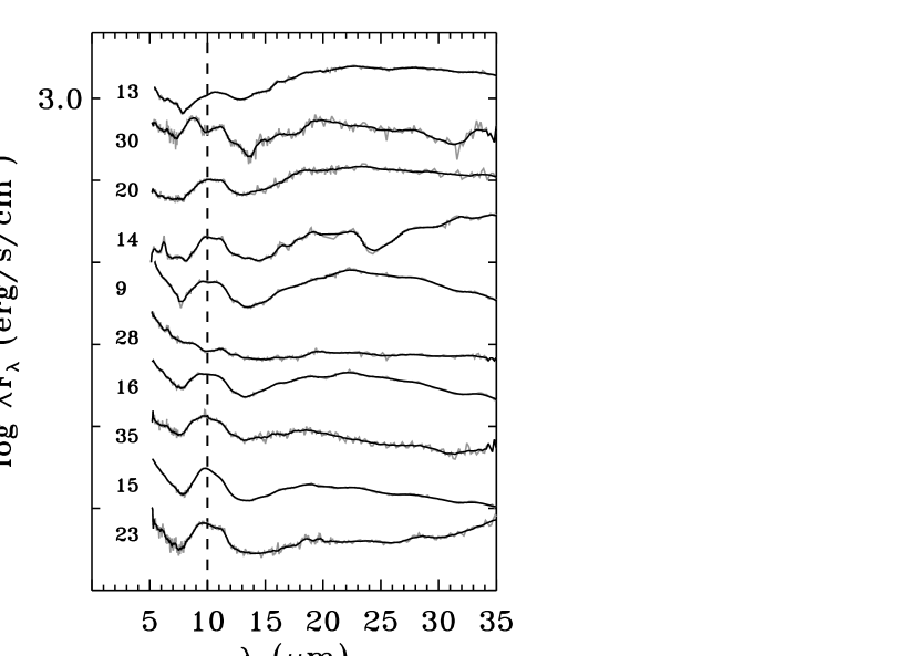
Figure 2: IRS spectra of the disks in the sample for which inner holes were not required to obtain a good SED fit organized from bottom to top with increasing SED slope $\alpha$. The thick and grey lines are the binned and original spectra, respectively and the numbers give their identifications in Table 1.

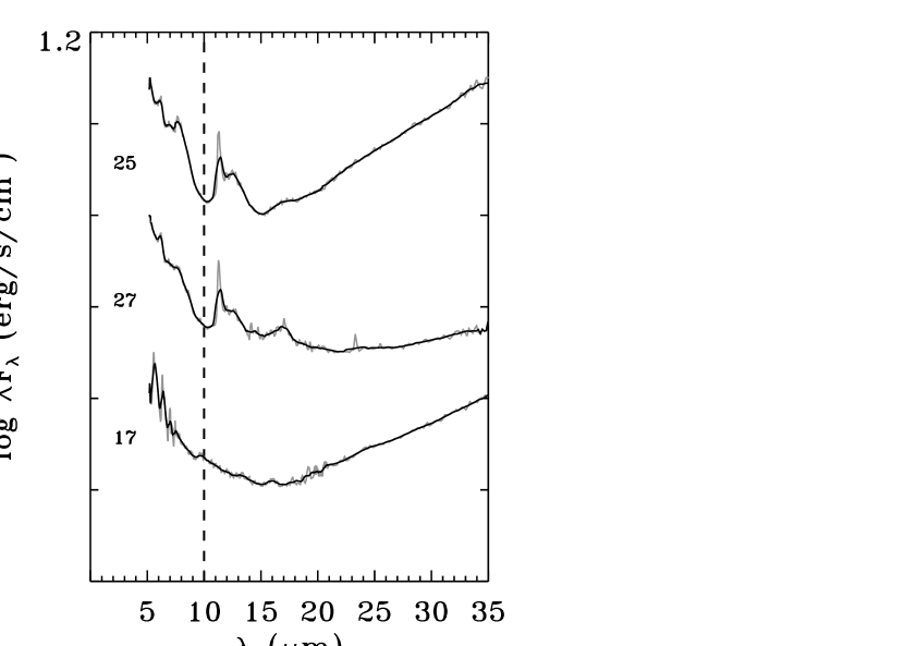
Figure 3: IRS spectra of the disks with potentially extended mid-IR emission from surrounding clouds ordered from bottom to top with growing stellar mass. Object 17 (Sz 84) is shown here as comparison due to its similar IRS spectrum, although it is classified as a cold disk. The thick and grey lines are the binned and original spectra, respectively and the numbers give their identifications in Table 1.

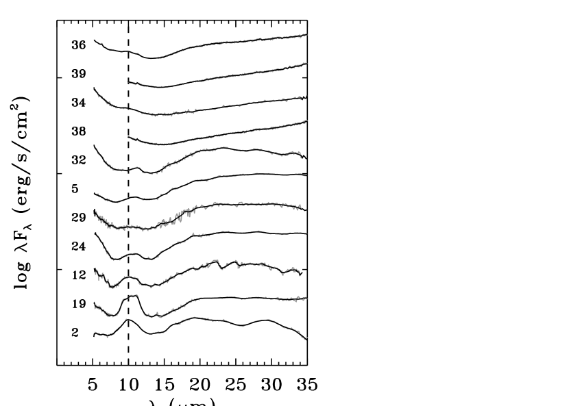
Figure 4: IRS spectra of the accreting cold disks in the sample ordered from bottom to top with growing inner hole radii. The thick and grey lines are the binned and original spectra, respectively and the numbers give their identifications in Table 1.

Figure 6: Spectral Energy Distributions of the eight close to edge-on disks (top) in the sample and the two extended sources (bottom). Points are observed fluxes from IRAC, MIPS and IRAM. The thick solid line is the IRS spectrum and the numbers give their identifications in Table 1.

Figure 10: Comparison between hole radii computed with the RADMC models (Dullemond & Dominik, 2004) and with the Robitaille et al. (2007) disk model grid. Even with the large scatter, both quantities are correlated, which shows that the derived disk hole radius is model independent to generally within a factor of 2-3.

Figure 11: Inner disk radius histograms for the cold disks in the sample. The cold disks predominantly have inner holes with radii smaller than 10 AU. Many of the cold disks in the literature have larger hole sizes.

Figure 12: Continuum subtracted PAH emission from object # 27. The vertical dashed lines show PAH features.

Figure 16: Correlation between hole size and disk mass. Dots and upper limits represent source with millimeter fluxes from this work while the diamonds are the cold disks with millimeter measured disk masses from Kim et al. (2009) and Brown et al. (2007). To minimize systematic differences, disk masses for sources from Kim et al. (2009) have been recalculated using the 1.3 mm fluxes in Andrews & Williams (2005) and the conversion in Section 4.1. The correlation has a Pearson’s correlation coefficient of 0.6 and is statistically significant on the 99% level including the upper limits and 90% level with only the detected sources. The systematically lower disk masses in this survey might explain the generally smaller hole sizes than previously published transitional disks.

Figure 17: Relationship between the size of the inner disk hole and the mass of the central star. Solid circles represent our sample while stars and diamonds are transitional disks from Brown et al. (2007) and Kim et al. (2009) respectively. The dotted line is the best linear fit to the data. The small crosses mark the semimajor axis of all exoplanets in the http://exoplanet.eu database as of December 2009, compared to the mass of their parent stars.

Figure 18: Relationship between the size of the inner disk hole and the intensity of the 10 $\mu$m feature. Solid, grey and open circles represent c2d accreting, non-accreting cold disks and objects for which we do not have yet accretion information, respectively.

References

- Acke & van den Ancker (2004) Acke, B. & van den Ancker, M. E. 2004, A&A, 426, 151
- Alcalá et al. (2008) Alcalá, J. M., Spezzi, L., Chapman, N., et al. 2008, ApJ, 676, 427
- Alexander et al. (2006) Alexander, R. D., Clarke, C. J., & Pringle, J. E. 2006, MNRAS, 369, 216
- Allers et al. (2006) Allers, K. N., Kessler-Silacci, J. E., Cieza, L. A., & Jaffe, D. T. 2006, ApJ, 644, 364
- André et al. (1990) André, P., Montmerle, T., Feigelson, E. D., & Steppe, H. 1990, A&A, 240, 321
- Andrews & Williams (2005) Andrews, S. M. & Williams, J. P. 2005, ApJ, 631, 1134
- Andrews & Williams (2007) Andrews, S. M. & Williams, J. P. 2007, ApJ, 671, 1800
- Andrews et al. (2009) Andrews, S. M., Wilner, D. J., Hughes, A. M., Qi, C., & Dullemond, C. P. 2009, ArXiv e-prints
- Artymowicz & Lubow (1994) Artymowicz, P. & Lubow, S. H. 1994, ApJ, 421, 651
- Artymowicz & Lubow (1996) Artymowicz, P. & Lubow, S. H. 1996, ApJ, 467, L77+
- Aspin et al. (1994) Aspin, C., Sandell, G., & Russell, A. P. G. 1994, A&AS, 106, 165
- Baraffe et al. (1998) Baraffe, I., Chabrier, G., Allard, F., & Hauschildt, P. H. 1998, A&A, 337, 403
- Beckwith et al. (1990) Beckwith, S. V. W., Sargent, A. I., Chini, R. S., & Guesten, R. 1990, AJ, 99, 924
- Bingham et al. (1994) Bingham, R. G., Gellatly, D. W., Jenkins, C. R., & Worswick, S. P. 1994, in Presented at the Society of Photo-Optical Instrumentation Engineers (SPIE) Conference, Vol. 2198, Society of Photo-Optical Instrumentation Engineers (SPIE) Conference Series, ed. D. L. Crawford & E. R. Craine, 56–64
- Bouwman et al. (2008) Bouwman, J., Henning, T., Hillenbrand, L. A., et al. 2008, ApJ, 683, 479
- Brown et al. (2007) Brown, J. M., Blake, G. A., Dullemond, C. P., et al. 2007, ApJ, 664, L107
- Brown et al. (2008) Brown, J. M., Blake, G. A., Qi, C., Dullemond, C. P., & Wilner, D. J. 2008, ApJ, 675, L109
- Brown et al. (2009) Brown, J. M., Blake, G. A., Qi, C., et al. 2009, ApJ, 704, 496
- Bryden et al. (1999) Bryden, G., Chen, X., Lin, D. N. C., Nelson, R. P., & Papaloizou, J. C. B. 1999, ApJ, 514, 344
- Calvet et al. (2002) Calvet, N., D’Alessio, P., Hartmann, L., et al. 2002, ApJ, 568, 1008
- Calvet et al. (2005) Calvet, N., D’Alessio, P., Watson, D. M., et al. 2005, ApJ, 630, L185
- Carpenter et al. (2009) Carpenter, J. M., Mamajek, E. E., Hillenbrand, L. A., & Meyer, M. R. 2009, ApJ, 705, 1646
- Chapman et al. (2009) Chapman, N. L., Mundy, L. G., Lai, S., & Evans, N. J. 2009, ApJ, 690, 496
- Chen et al. (2006) Chen, C. H., Sargent, B. A., Bohac, C., et al. 2006, ApJS, 166, 351
- Chiang & Murray-Clay (2007) Chiang, E. & Murray-Clay, R. 2007, Nature Physics, 3, 604
- Chiang & Goldreich (1997) Chiang, E. I. & Goldreich, P. 1997, ApJ, 490, 368
- Cieza et al. (2007) Cieza, L., Padgett, D. L., Stapelfeldt, K. R., et al. 2007, ApJ, 667, 308
- Cieza et al. (2010) Cieza, L. A., Schreiber, M. R., Romero, G. A., et al. 2010, ApJ, 712, 925
- Cieza et al. (2008a) Cieza, L. A., Swift, J. J., Mathews, G. S., & Williams, J. P. 2008a, ApJ, 686, L115
- Cieza et al. (2008b) Cieza, L. A., Swift, J. J., Mathews, G. S., & Williams, J. P. 2008b, ArXiv e-prints
- Clarke et al. (2001) Clarke, C. J., Gendrin, A., & Sotomayor, M. 2001, MNRAS, 328, 485
- Comerón et al. (2009) Comerón, F., Spezzi, L., & López Martí, B. 2009, A&A, 500, 1045
- Currie et al. (2009) Currie, T., Lada, C. J., Plavchan, P., et al. 2009, ApJ, 698, 1
- Dahm & Carpenter (2009) Dahm, S. E. & Carpenter, J. M. 2009, AJ, 137, 4024
- Dolidze & Arakelyan (1959) Dolidze, M. V. & Arakelyan, M. A. 1959, AZh, 36, 444
- Dullemond & Dominik (2004) Dullemond, C. P. & Dominik, C. 2004, A&A, 417, 159
- Dullemond & Dominik (2005) Dullemond, C. P. & Dominik, C. 2005, A&A, 434, 971
- Dullemond & Dominik (2008) Dullemond, C. P. & Dominik, C. 2008, A&A, 487, 205
- Dullemond et al. (2007) Dullemond, C. P., Hollenbach, D., Kamp, I., & D’Alessio, P. 2007, Protostars and Planets V, 555
- Ercolano et al. (2009) Ercolano, B., Clarke, C. J., & Robitaille, T. P. 2009, MNRAS, 394, L141
- Espaillat et al. (2007) Espaillat, C., Calvet, N., D’Alessio, P., et al. 2007, ApJ, 670, L135
- Espaillat et al. (2008) Espaillat, C., Calvet, N., Luhman, K. L., Muzerolle, J., & D’Alessio, P. 2008, ApJ, 682, L125
- Evans et al. (2009) Evans, N. J., Dunham, M. M., Jørgensen, J. K., et al. 2009, ApJS, 181, 321
- Evans et al. (2003) Evans, II, N. J., Allen, L. E., Blake, G. A., et al. 2003, PASP, 115, 965
- Fang et al. (2009) Fang, M., van Boekel, R., Wang, W., et al. 2009, A&A, 504, 461
- Flaherty et al. (2007) Flaherty, K. M., Pipher, J. L., Megeath, S. T., et al. 2007, ApJ, 663, 1069
- Forrest et al. (2004) Forrest, W. J., Sargent, B., Furlan, E., et al. 2004, ApJS, 154, 443
- Furlan et al. (2006) Furlan, E., Hartmann, L., Calvet, N., et al. 2006, ApJS, 165, 568
- Furlan et al. (2009) Furlan, E., Watson, D. M., McClure, M. K., et al. 2009, ApJ, 703, 1964
- Gagné et al. (2004) Gagné, M., Skinner, S. L., & Daniel, K. J. 2004, ApJ, 613, 393
- Geers et al. (2006) Geers, V. C., Augereau, J.-C., Pontoppidan, K. M., et al. 2006, A&A, 459, 545
- Geers et al. (2007a) Geers, V. C., Pontoppidan, K. M., van Dishoeck, E. F., et al. 2007a, A&A, 469, L35
- Geers et al. (2007b) Geers, V. C., van Dishoeck, E. F., Visser, R., et al. 2007b, A&A, 476, 279
- Getman et al. (2002) Getman, K. V., Feigelson, E. D., Townsley, L., et al. 2002, ApJ, 575, 354
- Gorti & Hollenbach (2009) Gorti, U. & Hollenbach, D. 2009, ApJ, 690, 1539
- Gutermuth et al. (2004) Gutermuth, R. A., Megeath, S. T., Muzerolle, J., et al. 2004, ApJS, 154, 374
- Habart et al. (2006) Habart, E., Natta, A., Testi, L., & Carbillet, M. 2006, A&A, 449, 1067
- Haisch et al. (2001) Haisch, Jr., K. E., Lada, E. A., & Lada, C. J. 2001, ApJ, 553, L153
- Hartigan (1993) Hartigan, P. 1993, AJ, 105, 1511
- Hartmann (2001) Hartmann, L. 2001, Accretion Processes in Star Formation
- Harvey et al. (2007) Harvey, P., Merín, B., Huard, T. L., et al. 2007, ApJ, 663, 1149
- Hauschildt et al. (1999) Hauschildt, P. H., Allard, F., Ferguson, J., Baron, E., & Alexander, D. R. 1999, ApJ, 525, 871
- Henning et al. (1993) Henning, T., Pfau, W., Zinnecker, H., & Prusti, T. 1993, A&A, 276, 129
- Herbig & Bell (1988) Herbig, G. H. & Bell, K. R. 1988, Catalog of emission line stars of the orion population : 3 : 1988 (Lick Observatory Bulletin, Santa Cruz: Lick Observatory, —c1988)
- Hernández et al. (2007) Hernández, J., Hartmann, L., Megeath, T., et al. 2007, ApJ, 662, 1067
- Hughes et al. (2009) Hughes, A. M., Andrews, S. M., Espaillat, C., et al. 2009, ApJ, 698, 131
- Hughes et al. (2007) Hughes, A. M., Wilner, D. J., Calvet, N., et al. 2007, ApJ, 664, 536
- Ireland & Kraus (2008) Ireland, M. J. & Kraus, A. L. 2008, ArXiv e-prints, 803
- Jayawardhana et al. (2006) Jayawardhana, R., Coffey, J., Scholz, A., Brandeker, A., & van Kerkwijk, M. H. 2006, ApJ, 648, 1206
- Jensen et al. (2009) Jensen, E. L. N., Cohen, D. H., & Gagné, M. 2009, ApJ, 703, 252
- Jørgensen et al. (2006) Jørgensen, J. K., Harvey, P. M., Evans, II, N. J., et al. 2006, ApJ, 645, 1246
- Jura et al. (2004) Jura, M., Chen, C. H., Furlan, E., et al. 2004, ApJS, 154, 453
- Kalas et al. (2008) Kalas, P., Graham, J. R., Chiang, E., et al. 2008, Science, 322, 1345
- Kenyon & Bromley (2009) Kenyon, S. J. & Bromley, B. C. 2009, ApJ, 690, L140
- Kenyon & Hartmann (1995) Kenyon, S. J. & Hartmann, L. 1995, ApJS, 101, 117
- Kessler-Silacci et al. (2006) Kessler-Silacci, J., Augereau, J.-C., Dullemond, C. P., et al. 2006, ApJ, 639, 275
- Kim et al. (2009) Kim, K. H., Watson, D. M., Manoj, P., et al. 2009, ApJ, 700, 1017
- Koike et al. (1993) Koike, C., Shibai, H., & Tuchiyama, A. 1993, MNRAS, 264, 654
- Kraus et al. (2009) Kraus, A. L., Ireland, M. J., Martinache, F., & Lloyd, J. P. 2009, in American Institute of Physics Conference Series, Vol. 1094, American Institute of Physics Conference Series, ed. E. Stempels, 453–456
- Krautter et al. (1997) Krautter, J., Wichmann, R., Schmitt, J. H. M. M., et al. 1997, A&AS, 123, 329
- Kreysa et al. (2002) Kreysa, E., Gemünd, H.-P., Raccanelli, A., Reichertz, L. A., & Siringo, G. 2002, in American Institute of Physics Conference Series, Vol. 616, Experimental Cosmology at Millimetre Wavelengths, ed. M. de Petris & M. Gervasi, 262–269
- Kurosawa et al. (2006) Kurosawa, R., Harries, T. J., & Symington, N. H. 2006, MNRAS, 370, 580
- Lada et al. (2006) Lada, C. J., Muench, A. A., Luhman, K. L., et al. 2006, AJ, 131, 1574
- Lagrange et al. (2009) Lagrange, A.-M., Gratadour, D., Chauvin, G., et al. 2009, A&A, 493, L21
- Lahuis et al. (2007) Lahuis, F., van Dishoeck, E. F., Blake, G. A., et al. 2007, ApJ, 665, 492
- Leggett (1992) Leggett, S. K. 1992, ApJS, 82, 351
- Liu et al. (1980) Liu, C.-P., Zhang, C.-S., & Kimura, H. 1980, Acta Astronomica Sinica, 21, 354
- Low et al. (2005) Low, F. J., Smith, P. S., Werner, M., et al. 2005, ApJ, 631, 1170
- Luhman et al. (2003) Luhman, K. L., Briceño, C., Stauffer, J. R., et al. 2003, ApJ, 590, 348
- Luhman et al. (1998) Luhman, K. L., Briceno, C., Rieke, G. H., & Hartmann, L. 1998, ApJ, 493, 909
- Marois et al. (2008) Marois, C., Macintosh, B., Barman, T., et al. 2008, Science, 322, 1348
- McClure (2009) McClure, M. 2009, ApJ, 693, L81
- Merín et al. (2008) Merín, B., Jørgensen, J., Spezzi, L., et al. 2008, ApJS, 177, 551
- Montes et al. (1997) Montes, D., Martin, E. L., Fernandez-Figueroa, M. J., Cornide, M., & de Castro, E. 1997, A&AS, 123, 473
- Mora et al. (2001) Mora, A., Merín, B., Solano, E., et al. 2001, A&A, 378, 116
- Morales et al. (2009) Morales, F. Y., Werner, M. W., Bryden, G., et al. 2009, ApJ, 699, 1067
- Muench et al. (2007) Muench, A. A., Lada, C. J., Luhman, K. L., Muzerolle, J., & Young, E. 2007, AJ, 134, 411
- Muzerolle et al. (2010) Muzerolle, J., Allen, L. E., Megeath, S. T., Hernández, J., & Gutermuth, R. A. 2010, ApJ, 708, 1107
- Muzerolle et al. (2009) Muzerolle, J., Flaherty, K., Balog, Z., et al. 2009, ApJ, 704, L15
- Muzerolle et al. (2003) Muzerolle, J., Hillenbrand, L., Calvet, N., Briceño, C., & Hartmann, L. 2003, ApJ, 592, 266
- Najita et al. (2007) Najita, J. R., Strom, S. E., & Muzerolle, J. 2007, MNRAS, 378, 369
- Natta et al. (2004) Natta, A., Testi, L., Muzerolle, J., et al. 2004, A&A, 424, 603
- Nguyen et al. (2009) Nguyen, D. C., Scholz, A., van Kerkwijk, M. H., Jayawardhana, R., & Brandeker, A. 2009, ApJ, 694, L153
- Nuernberger et al. (1997) Nuernberger, D., Chini, R., & Zinnecker, H. 1997, A&A, 324, 1036
- Oliveira et al. (2009) Oliveira, I., Merín, B., Pontoppidan, K. M., et al. 2009, ApJ, 691, 672
- Oliveira et al. (2010) Oliveira, I., Pontoppidan, K. M., Merín, B., et al. 2010, ApJ, 714, 778
- Olofsson et al. (2009) Olofsson, J., Augereau, J., van Dishoeck, E. F., et al. 2009, A&A, 507, 327
- Osterloh & Beckwith (1995) Osterloh, M. & Beckwith, S. V. W. 1995, ApJ, 439, 288
- Padgett et al. (1999) Padgett, D. L., Brandner, W., Stapelfeldt, K. R., et al. 1999, AJ, 117, 1490
- Padgett et al. (2006) Padgett, D. L., Cieza, L., Stapelfeldt, K. R., et al. 2006, ApJ, 645, 1283
- Pascucci & Sterzik (2009) Pascucci, I. & Sterzik, M. 2009, ApJ, 702, 724
- Piétu et al. (2006) Piétu, V., Dutrey, A., Guilloteau, S., Chapillon, E., & Pety, J. 2006, A&A, 460, L43
- Pollack et al. (1996) Pollack, J. B., Hubickyj, O., Bodenheimer, P., et al. 1996, Icarus, 124, 62
- Pontoppidan et al. (2008) Pontoppidan, K. M., Blake, G. A., van Dishoeck, E. F., et al. 2008, ApJ, 684, 1323
- Pott et al. (2010) Pott, J., Perrin, M. D., Furlan, E., et al. 2010, ApJ, 710, 265
- Preibisch et al. (2003) Preibisch, T., Stanke, T., & Zinnecker, H. 2003, A&A, 409, 147
- Preibisch & Zinnecker (2001) Preibisch, T. & Zinnecker, H. 2001, AJ, 122, 866
- Quillen et al. (2004) Quillen, A. C., Blackman, E. G., Frank, A., & Varnière, P. 2004, ApJ, 612, L137
- Reipurth et al. (1996) Reipurth, B., Pedrosa, A., & Lago, M. T. V. T. 1996, A&AS, 120, 229
- Robitaille et al. (2007) Robitaille, T. P., Whitney, B. A., Indebetouw, R., & Wood, K. 2007, ApJS, 169, 328
- Salyk et al. (2009) Salyk, C., Blake, G. A., Boogert, A. C. A., & Brown, J. M. 2009, ApJ, 699, 330
- Schwartz (1977) Schwartz, R. D. 1977, ApJS, 35, 161
- Sicilia-Aguilar et al. (2005) Sicilia-Aguilar, A., Hartmann, L. W., Hernández, J., Briceño, C., & Calvet, N. 2005, AJ, 130, 188
- Sicilia-Aguilar et al. (2010) Sicilia-Aguilar, A., Henning, T., & Hartmann, L. W. 2010, ApJ, 710, 597
- Sicilia-Aguilar et al. (2008) Sicilia-Aguilar, A., Henning, T., Juhász, A., et al. 2008, ApJ, 687, 1145
- Siess et al. (2000) Siess, L., Dufour, E., & Forestini, M. 2000, A&A, 358, 593
- Skrutskie et al. (1990) Skrutskie, M. F., Dutkevitch, D., Strom, S. E., et al. 1990, AJ, 99, 1187
- Spezzi et al. (2008) Spezzi, L., Alcalá, J. M., Covino, E., et al. 2008, ApJ, 680, 1295
- Spezzi et al. (2010) Spezzi, L., Merín, B., Oliveira, I., van Dishoeck, E. F., & Brown, J. M. 2010, A&A, 513, A38+
- Strom et al. (1989) Strom, K. M., Strom, S. E., Edwards, S., Cabrit, S., & Skrutskie, M. F. 1989, AJ, 97, 1451
- Sylvester et al. (1996) Sylvester, R. J., Skinner, C. J., Barlow, M. J., & Mannings, V. 1996, MNRAS, 279, 915
- Tanaka et al. (2005) Tanaka, H., Himeno, Y., & Ida, S. 2005, ApJ, 625, 414
- Tielens (2008) Tielens, A. G. G. M. 2008, ARA&A, 46, 289
- van Boekel et al. (2005) van Boekel, R., Min, M., Waters, L. B. F. M., et al. 2005, A&A, 437, 189
- Varnière et al. (2006) Varnière, P., Blackman, E. G., Frank, A., & Quillen, A. C. 2006, ApJ, 640, 1110
- Walawender et al. (2005) Walawender, J., Bally, J., & Reipurth, B. 2005, AJ, 129, 2308
- Watson et al. (2009) Watson, D. M., Leisenring, J. M., Furlan, E., et al. 2009, ApJS, 180, 84
- Weidenschilling (2000) Weidenschilling, S. J. 2000, Space Science Reviews, 92, 295
- Weingartner & Draine (2001) Weingartner, J. C. & Draine, B. T. 2001, ApJ, 548, 296
- White & Basri (2003) White, R. J. & Basri, G. 2003, ApJ, 582, 1109
- White & Hillenbrand (2004) White, R. J. & Hillenbrand, L. A. 2004, ApJ, 616, 998
- Wuchterl et al. (2000) Wuchterl, G., Guillot, T., & Lissauer, J. J. 2000, Protostars and Planets IV, 1081
- Zylka (1998) Zylka, R. 1998, MOPSI Users Manual, IRAM, Grenoble