Abstract

An emission tomography of laser-induced plasmas employed in the laser induced breakdown spectroscopy (LIBS) requires long signal integration times during which the plasma cannot be considered stationary. To reduce the integration time, it is proposed to measure a plasma absorption in parallel rays with an aperture that collects light coming from large fractions of the plasma plume at each aperture position. The needed spatial resolution is achieved by a special numerical data processing. Another advantage of the proposed procedure is that inexpensive linear CCD or non-discrete (PMT, photodiode) detectors can be used instead of costly 2-dimensional detectors.

1 Large apertures and the Abel inversion

It is assumed that a plasma plume created by a laser ablation is axially symmetric (the symmetry axis coincides with the laser ray). Let the coordinate system be set so that the symmetry axis is the $z-$ axis. Then the emissivity is a function $\varepsilon=\varepsilon(r,z,t,\nu)$ where $r=(y^{2}+x^{2})^{1/2}$, $t$ is the time, and $\nu$ is the frequency. A measured quantity is the intensity $I(y,z,t,\nu)$ of light per unit time and unit frequency along the rays through an infinitesimal area element $\Delta A=\Delta y\Delta z$ centered at the point $(0,y,z)$ that are in a narrow solid angle $\Delta\Omega$ about the line parallel to the $x-$axis:

$$I(y,z,t,\nu)=\Delta A\Delta\Omega\int_{-\infty}^{\infty}dx\,\varepsilon\Bigl{(}\sqrt{y^{2}+x^{2}},z,t,\nu\Bigr{)}=2\Delta A\Delta\Omega\int_{y}^{\infty}\frac{dr\,r\,\varepsilon(r,z,t,\nu)}{\sqrt{r^{2}-y^{2}}}\,.$$ (1)

It is well-known that Eq.(1) can be solved for $\varepsilon(r,z,t)$ by the Abel inversion [1, 2]. A plasma plume has a finite size that determines a cut-off of the infinite integration limits in (1). Equation (1) is valid only for infinitesimal $\Delta A$ and $\Delta\Omega$ and so is the approximation of the parallel rays that allows for the subsequent Abel inversion. In typical LIBS experiments, the smallness of $\Delta A$ is provided by a narrow spectrometer slit and small pixel size of a detector, while $\Delta\Omega$ is small due to a low acceptance angle of a spectrometer (high $f-$numbers). To compensate for small factors $\Delta A$ and $\Delta\Omega$, a long integration time $T$ is used to collect enough energy $E=\int_{0}^{T}dtI(y,z,t,\nu)$ of photons emitted by the plasma along parallel rays. A typical integration time in LIBS plasma experiments is $T\sim 1\,\mu s$ or even higher. If the plasma is not stationary during the time $T$, the collected data correspond to a time-averaged intensity and the reconstructed emissivity may not be accurate. This is especially relevant for studying elemental contents of plasmas expanding into an ambient gas because of percolation processes at a rapidly moving plasma-gas interface. Numerical simulations of LIBS plasma dynamics show that this is often the case, especially for earlier stages of the plasma evolution (see, e.g., [3, 4]).

Here it is proposed to increase an aperture through which parallel rays are collected in order to reduce the integration time so that the observed intensity is:

$$I_{E}(y)=\Delta z\Delta\Omega\int_{y-\Delta}^{y+\Delta}du\int_{-\infty}^{\infty}dx\,\varepsilon\Bigl{(}\sqrt{u^{2}+x^{2}}\Bigr{)}\equiv\int_{y-\Delta}^{y+\Delta}duI(u)\,.$$ (2)

where the dependence on $z$, $t$, and $\nu$ is now suppressed as it is irrelevant for the discussion. Equation (2) states that all photons traveling parallel to the $x-$axis and coming through a rectangular aperture of an infinitesimal height $\Delta z$ and finite width $2\Delta$ and centered at a distance $y$ from the $x-$axis are collected. An experimental setup to which Eq. (2) applies is discussed below (see Fig. 1). In the limit $\Delta=\Delta y/2\rightarrow 0$, Eq. (2) turns into Eq.(1). So, the signal can be amplified roughly by the factor of $2\Delta/\Delta y$. A spatial resolution $\Delta y$ in a typical experimental setup [5, 6, 7] is determined by a pixel size of a camera used to register $I(y)$, $\Delta y\sim 0.02\,mm$. If the aperture width is taken to be of a typical size of a LIBS plasma plume, $2\Delta\sim 2\,mm$, up to two orders in magnitude of the signal strength can be gained. How is then the spatial resolution restored? It is proved below that, given a function $I_{E}(y)$, the function $I(y)$ can be uniquely determined from (2) for any $\Delta$, provided $I(y)$ satisfies the condition that $I(y)$ vanishes for $|y|>D$ for some $D$, which is always the case for a physical $I(y)$ because a plasma plume has a finite size. Thus, the proposed procedure entails:

(i) Taking intensity measurements of $I_{E}(y)$ at a set of positions $y=y_{n}$;
(ii) Reconstructing the intensities $I(y_{n})$ from the data $I_{E}(y_{n})$;
(iii) The Abel inversion for $I(y_{n})$.

A key issue for the data collection (i) is to separate parallel and angled rays passing through the aperture. Note that for a non-infinitesimal $\Delta$ there should be rays coming through the aperture at a finite angle to its normal and, hence, $\Delta\Omega$ can no longer be considered infinitesimal, thus, invalidating the approximation of parallel rays in (2). This is indeed true if the plasma emission is collected by the slit. The problem can be avoided if the collimated light absorbed by the plasma is measured. An experimental setup to achieve this goal is presented in Section 2 (see Fig. 1).

An explicit algorithm to carry out (ii) is given in Section 3. The spatial resolution is determined by the difference $\Delta_{s}=y_{n}-y_{n-1}$ in positions of the center of the aperture. Numerical simulations with synthetic data representative for LIBS plasmas are presented in Section 4. There is a variety of numerical methods available to carry out the Abel inversion (see, e.g., [8], and more recent applications to LIBS plasmas [6, 7]). So the part (iii) will not be discussed here.

2 Plasma absorption experiments

The proposed hypothetical experimental setup is shown in Fig. 1.

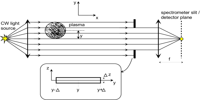
Figure 1: An experimental setup for plasma absorption measurements with a large aperture. A CW light source is in focus of a lens to create a flux of parallel rays. A plasma plume with the symmetry axis normal to the figure plane is illuminated by the parallel rays. The parallel flux across a rectangular aperture is focused onto a detector (a spectrometer slit or CCD camera). The aperture plane is normal to the flux. It is positioned at a distance large enough to neglect contributions of the plasma plume emission. The aperture geometry is depicted in the inset at the bottom of the figure. The height $\Delta z$ is small enough to neglect variations of the plasma absorption along the $z-$direction. The aperture width $2\Delta$ can be of the size of the plasma plume or larger. The intensity in parallel rays is measured for different values of $y$, the distance between the plasma symmetry axis and the optical axis of the system. Measurements at a fixed value of $y$ have no spatial resolution by themselves if $\Delta$ is large. The spatial resolution is restored by a numerical processing of data collected at different values of $y$.

A point light source is placed in a focus of lens so that after the lens the light propagates parallel to its optical axis. The light goes through a plasma plume. Some of the photons will be absorbed by the plasma and then re-emitted. However the re-emission occurs in the whole solid angle of $4\pi$, i.e., the absorbed light no longer contributes to the parallel flux. Since the intensity of the plasma radiation is inversely proportional to the squared distance from the plasma center, by placing the aperture at a distance large enough from the plasma center the contribution of the plasma radiation through the aperture becomes negligible as compared to that of the parallel light. The plasma emissivity, $\varepsilon(r)$, is determined by the absorption coefficient $\kappa(r)$ and the black body radiation function $B(r)$, $\varepsilon(r)=\kappa(r)B(r)$, provided, of course, that the plasma is at a local thermodynamic equilibrium (see, e.g., [9]). So, by measuring the difference between the fluxes in parallel rays piercing through the aperture area $\Delta A=2\Delta z\Delta$ with and without the plasma plume inserted, the contribution of the plasma emissivity expressed as the attenuation of the parallel flux across $\Delta A$ is obtained. The plasma plume symmetry axis is positioned at a distance $y$ from the optical axis of the right lens (the lens behind the slit). The center of the aperture also lies on this optical axis. The parallel rays that came through the aperture are focused on the spectrometer slit. In this setting, the spectrometer-detector combination is only used to achieve the spectral resolution because all the light that came through the aperture of width $2\Delta$ is focused to a single point of the spectrometer slit. Thus, there is no spatial resolution in measurements at a fixed value of $y$. An analogy to the data collection in the aforementioned emission experiments, e.g. [6, 7], would correspond to the case when the right lens is removed in Fig. 1 so that the light is collected by all pixels of a detector evenly distributed along the spectrometer slit and both the spatial and spectral resolutions are achieved. In contrast, here all the light is focused onto a single pixel by the right lens in Fig. 1. Thus, the signal amplification is achieved at the price of loosing the spatial resolution in measurements. However, as noted before, the spatial resolution is restored by a numerical data processing. It is noteworthy that 2D CCD detectors are no longer required to spatially resolve the plasma radiation. Inexpensive linear detectors (if the spectral dimension is to be retained) or photomultiplier tubes (PMT) can be used instead.

The measurements of $I_{E}(y)$ are taken at different positions of the center of the aperture $y=y_{n}=n\Delta_{s}$, $n=0,\pm 1,\pm 2,...,\pm N$, where $\Delta_{s}$ is the slit center displacement relative to the plasma plume symmetry axis (it is more convenient to create plasma plumes at different positions $y_{n}$). The step $\Delta_{s}$ can be made as small as desired (or possible to achieve). The limiting positions $y=\pm N\Delta_{s}$ are chosen so that the studied plasma plume absorption does not contribute to the parallel flux through the aperture (i.e., $N\Delta_{s}-\Delta$ exceeds the plasma plume radius).

The light source for absorption measurements must be bright enough, i.e., comparable to the plasma own spectral emission, otherwise the gain by the large aperture is rendered useless by a flux weaker than that of the plasma emission. Possible solutions of this problem are as follows. First, another laser-induced plasma plume can be used as the point light source. It is just as bright as the studied plasma plume, has a broadband spectrum, and a short pulse duration suitable for time-resolved measurements. Plasma plumes as the light source for absorption measurements have been used in experiments reported in [10]. Second, super-continuum white light lasers [11] with a broadband output spectrum can be used as a light source for absorption measurements. Finally, if the spectral resolution is not relevant, a single frequency laser can be used to study plasma emissivity at a particular frequency that coincides with one of the plasma emissivity spectral lines [12]. The problem of an insufficient spectral brightness is also resolved in this case.

3 The reconstruction algorithm

The integral equation (2) is a linear equation. So its solution is the sum of a general solution $I_{0}(y)$ of the homogeneous equation (when $I_{E}=0$) and a particular solution of the non-homogeneous equation (2). It is assumed that $I_{E}(y)$ cannot be a non-vanishing constant (a plasma plume has a finite size). Differentiating Eq. (2) with respect to $y$ and shifting the argument $y\rightarrow y-\Delta$, one infers:

$$I(y)=I(y-2\Delta)+I^{\prime}_{E}(y-\Delta)\,.$$ (3)

If $I_{E}=0$, then $I(y)=I_{0}(y)=I_{0}(y-2\Delta)$ is a periodic function that is a linear combination of $\exp(i\pi ky/\Delta)$ for $k=\pm 1,\pm 2,...$ (the case $k=0$ is not possible for $I_{E}=0$ in Eq. (2)). By physical boundary conditions, $I_{E}(y)=I(y)=0$ for all $|y|>D$ and some $D$. No periodic $I_{0}(y)$ satisfies this condition. Thus, under this boundary condition, $I(y)$ is uniquely recovered from $I_{E}(y)$. The solution can be written in the form:

$$I(y)=\frac{1}{2}\sum_{q=0}^{\infty}\Bigl{\{}I^{\prime}_{E}\Bigl{(}y-\Delta(2q+1)\Bigr{)}-I_{E}^{\prime}\Bigl{(}y+\Delta(2q+1)\Bigr{)}\Bigr{\}}\,.$$ (4)

It can be verified by its substitution into the right side of Eq. (2). To understand the structure of the solution (4), it might be instructive to work out a simple analytic example of reconstructing $I(y)=A=const$ for $|y|\leq\Delta$ and $I(y)=0$ otherwise. The function $I_{E}(y)$ is easy to compute by Eq. (2), $I_{E}(y)=A(2\Delta-|y|)$ if $|y|\leq 2\Delta$ and $I_{E}(y)=0$ otherwise. Then $I_{E}(y)$ can be substituted into the right side of Eq. (4) to see how $I(y)$ is recovered through cancellations in the sum. In this simple case, the function $I(y)$ is reconstructed in the interval $|y|\leq\Delta$ by the first term $q=0$ in the sum (4). The other terms vanish for $|y|\leq\Delta$ and are needed to make $I(y)=0$ for $|y|>\Delta$. So, for a plasma plume of a radius $R$, only first $R/\Delta$ terms are needed to reconstruct $I(y)$ in the interval $|y|\leq R$.

Put $\Delta=m\Delta_{s}$ for some integer $m$. Suppose that the data function $I_{E}(y)$ is taken at the grid points $y_{n}=n\Delta_{s}$ where $n=-N,-N+1,...,N-1,N$ so that $I_{E}(y)=0$ for all $y\leq y_{-N}$ and $y\geq y_{N}$. Consequently, this implies that $I(y)=0$ for all $y\leq y_{-N+m}$ and $y\geq y_{N-m}$. The number $N$ is chosen so that $(N-m)\Delta_{s}$ exceeds the plasma plume radius. In practice, the data collection should simply start at $|y|$ large enough to see no signal from the plasma. Then $y$ is changed with the step $\Delta_{s}$ until the signal vanishes again. Equation (3) becomes the recurrence relation:

$$I(y_{n})=I(y_{n-2m})+I^{\prime}_{E}(y_{n-m})\,.$$ (5)

With the boundary conditions imposed on the data set, it follows from the first $2m$ relations in (5) that

$$I(y_{n})=I^{\prime}_{E}(y_{n-m})\,,\quad n=-N+m+1,...,-N+3m\,.$$ (6)

The values $I(y_{n})$ for $n>-N+3m$ are then determined recursively by (5) because the preceding values $I(y_{n-2m})$ needed to initiate the recurrence relation (5) are now known from (6). The remaining problem is to calculate $I_{E}^{\prime}(y_{n})$ from the set $I_{E}(y_{n})$.

Let $\tilde{I}_{E}(k)=\int dyI_{E}(y)e^{iky}$ be the Fourier transform of $I_{E}(y)$. The Fourier transform of $I_{E}^{\prime}(y)$ is $ik\tilde{I}_{E}(k)$. Thus the values $I^{\prime}_{E}(y_{n})$ can be found by a discrete Fourier transform:

$$I_{E}(y_{n})\stackrel{{\scriptstyle F}}{{\longrightarrow}}\tilde{I}_{E}(k_{n})\longrightarrow ik_{n}\tilde{I}_{E}(k_{n})\stackrel{{\scriptstyle F^{-1}}}{{\longrightarrow}}I^{\prime}_{E}(y_{n})\,,$$ (7)

where $F$ implies taking the fast Fourier transform of the data set $I_{E}(y_{n})$ to obtain the set $\tilde{I}_{E}(k_{n})$, and $F^{-1}$ is the inverse of $F$. For analytic functions, the accuracy of a numerical differentiation by the spectral (Fourier) method is superior to any finite differencing method [13]. The spatial resolution of the reconstructed intensities $I(y_{n})$ is determined by $\Delta_{s}$. It could even be better than in conventional settings where spectrometers with a pixel detector are used for the spatial resolution, provided it is possible to achieve $\Delta_{s}$ smaller than a spectrometer pixel size.

4 Numerical simulations with synthetic data

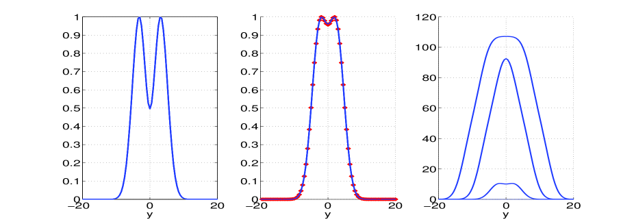
Figure 2: Left panel: The emissivity as a function of $r=|y|$ (the horizontal axis) as described in the text (arbitrary units). The plasma radius is roughly $R=10$. Middle panel: The intensity in parallel rays $I(y)$ calculated by Eq. (1) with the factor $\Delta A\Delta\Omega$ omitted. It is normalized so that its maximal value is one. The (red) dots indicate the values $I(y_{n})$ reconstructed from $I_{E}(y_{n})$ for $\Delta=R$ by the data processing algorithm of Section 3. Right panel: The intensities $I_{E}(y)$ for three different aperture widths. The upper, middle, and lower curves are the graphs of $I_{E}(y)$ computed by Eq. (2) with $\Delta=R$, $\Delta=R/2$, and $\Delta=R/10$, respectively.

The emissivity is taken in the form $\varepsilon(r)=\varepsilon_{0}\exp(-r^{2}/2\sigma^{2})(a-\cos(br))$ which resembles the emissivity profile typically observed in LIBS plasmas [7]. The parameters are chosen as $\varepsilon_{0}=1$, $\sigma=3$, $a=1.4$, and $b=0.5$ (arbitrary units). The graph of $\varepsilon(r)$ is shown in the left panel of Fig. 2. As seen from the figure, the plasma plume radius can be set as $R=10$ in these units. The intensity $I(y)$ in parallel rays is calculated by means of Eq. (1) (the geometrical factor $\Delta A\Delta\Omega$ is omitted). It is shown as the solid (blue) curve in the middle panel of Fig. 2. The function $I_{E}(y)$ calculated by means of Eq. (2) is shown in the right panel of Fig. (2). The top curve corresponds to the aperture width $2\Delta=2R$. For the middle curve, the aperture width is reduced twice $\Delta=R/2$, and the bottom curve corresponds to $\Delta=R/10$. In the conventional experimental settings, about $10$ to $20$ measurement across the plasma diameter are taken. So the bottom curve is representative for this case. A few remarks are in order. First, a significant gain in the signal amplitude is evident for the wide aperture. Second, the function $I_{E}(y)$ has support twice as wide as the plasma diameter if $2\Delta=2R$ because for $R<|y|<2R$ no parallel ray comes through the plasma, but the aperture centered at such $y$ can still capture parallel rays coming through the plasma. So the spatial resolution seems to be lost in the data $I_{E}(y)$. Third, the maximal amplitude of $I_{E}(y)$ cannot increase any further if $2\Delta>2R$. So, the aperture width equal to the plasma size gives the maximal amplification of the signal.

To illustrate the restoration of the spatial resolution, the function $I_{E}(y)$ is sampled at $y=y_{n}=n\Delta_{s}$ where $\Delta_{s}=R/20$. For the synthetic data $I_{E}(y_{n})$ when $2\Delta=2R$, a discrete Fourier transform is carried out to compute $I^{\prime}_{E}(y_{n})$ as specified in (7). The Fast Fourier Transform Matlab package has been used for this purpose. The values $I(y_{n})$ are recovered by means of the recurrence relation (5) with the initial conditions (6). They are shown by the (red) dots in the middle panel of Fig. 2. The dots lie on the graph of $I(y)$, i.e., the reconstruction is highly accurate. Naturally, the accuracy of the emissivity reconstruction from the data $I(y_{n})$ would then be fully determined by the accuracy of a particular Abel inversion algorithm [8].

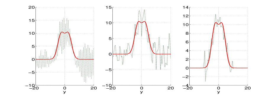
Figure 3: Noise effects on the reconstruction algorithm. The solid (red) curves on each panel is the graph of $I(y)$ as in the middle panel of Fig. 2 but without normalization on its maximal value. The dotted curves are the graphs of the reconstructed $I(y)$ from the ”noisy” data $I_{E}(y)$ as explained in the text for $\Delta=R/10$ (left panel), $\Delta=R/2$ (middle panel), and $\Delta=R$ (right panel). The signal-to-noise ratio is $S=0.7$, $S=2.9$, and $S=3.1$, respectively, in these three cases.

The proposed scheme can also be used to improve the signal to noise ratio when the integration time is fixed. In a typical LIBS experiment, the intensity data are collected from repeatedly created plasma plumes. The power of a laser pulse used for ablation varies from pulse to pulse, a material surface on which the ablation process takes place is not ideal, etc. All these effects generate a noise in $\varepsilon(r)$ and, hence, in $I(y)$. As an example, a white noise $\eta(y)$ has been added to $I(y)\rightarrow I_{\eta}(y)=I(y)+\eta(y)$. The values of $I_{E}(y)$ have been calculated by Eq. (2) with $I_{\eta}(y)$ for 50 samples of $\eta(y)$, and the result has been averaged. Then the reconstruction algorithm has been applied to recover $I(y)$ from the ”noisy” data $I_{E}(y)$. Figure 3 shows the graphs of the reconstructed functions $I(y)$ (dotted curves) for $\Delta=R/10$ (left panel), $\Delta=R/2$ (middle panel), and $\Delta=R$ (right panel). The solid (red) curve in each panel is the actual intensity $I(y)$ corresponding to the emissivity shown in the left panel of Fig. 2. In contrast to $I(y)$ depicted in the middle panel of Fig. 2, here $I(y)$ is given without the normalization on its maximal value, i.e., as defined by Eq. (1) without the factor $\Delta A\Delta\Omega$. The signal-to-noise ratio $S=I_{m}/\sigma$, where $\sigma$ is the standard deviation of the white noise and $I_{m}$ is the averaged signal amplitude near its maximum, is $S=0.7$, $S=2.9$, and $S=3.1$ for the above three values of $\Delta$, respectively. The increase of the signal-to-noise ratio in the reconstruction of $I(y)$ is self-evident.

References

- [1] A. C. Eckrbeth, Laser diagnostic for combustion temperature and species, (Gordon & Breach, Amsterdam, 1996)
- [2] H. R. Griem, Principles of plasma spectroscopy (Cambridge University Press, Cambridge, 1997)
- [3] A. Casavola, G. Colonna, and M. Capitelli, Appl. Surf. Sci. 208-209, 559 (2003)
- [4] M. Capitelli, F. Capitelli, and A. Eletskii, Spectrochim. Acta B 56, 567 (2001)
- [5] J. W. Olesik and G. M. Hieftje, Anal. Chem. 57, 2049 (1985)
- [6] R. Álvarez, A. Roberto, M. C. Quintero, Spectrochim. Acta B 57, 1665 (2002)
- [7] J. A. Aguilera, C. Aragón, and J. Bengoechea, Appl. Optics 42, 5938 (2003)
-
[8]
W. Lochte-Holtgreven, in:
Plasma diagnostics, ed. W. Lochte-Holtgreven
(North-Holland Pub. Co., Amsterdam, 1968), p. 135;
J.D. Algeo and M.B. Denton, Appl. Spectrosc. 35, 35 (1981);
W. R. Wing and R. V. Neidigh, Am. J. Phys. 39, 760 (1971);
R.N. Bracewell, The Fourier transform and its applications (McGraw-Hill Book Co., New York, 1965);
D.R. Keefer, L. Smith, and S.J. Sudhasanan, Abel inversion using transforms techniques (Univ. of Tennessee Space Institute, Tullahoma, 1986) - [9] Ya. B. Zel’dovich and Yu. P. Raizer, Physics of shock waves and high temperature hydrodynamics phenomena (Academic Press, New York, 1966)
- [10] I. B. Gornushkin, C. L. Stevenson, G. Galbács, B. W. Smith, and J. D. Winefordner, Appl. Spectrosc. 57, 1442 (2003)
- [11] A description of such lasers can be found in: http://www.nktphotonics.com
- [12] I. B. Gornushkin, B. W. Smith, N. Omenetto, and J. D. Winefordner, Spectrochim. Acta B 54, 1207 (1999)
-
[13]
B. Fornberg, A practical guide to pseudospectral
methods (Cambridge University Press, Cambridge,
1996);
J.P. Boyd, Chebyshev and Fourier spectral methods (Springer-Verlag, New York, 1989);
J.S. Hesthaven, S. Gottlieb, and D. Gottlieb, Spectral Methods for Time-Dependent Problems (Cambridge University Press, Cambridge, 2007).