Fully automatic extraction of salient objects from videos in near real-time

Abstract

Automatic video segmentation plays an important role in a wide range of computer vision and image processing applications. Recently, various methods have been proposed for this purpose. The problem is that most of these methods are far from real-time processing even for low-resolution videos due to the complex procedures. To this end, we propose a new and quite fast method for automatic video segmentation with the help of 1) efficient optimization of Markov random fields with polynomial time of number of pixels by introducing graph cuts, 2) automatic, computationally efficient but stable derivation of segmentation priors using visual saliency and sequential update mechanism, and 3) an implementation strategy in the principle of stream processing with graphics processor units (GPUs). Test results indicates that our method extracts appropriate regions from videos as precisely as and much faster than previous semi-automatic methods even though any supervisions have not been incorporated.

1 Introduction

Extracting important (or meaningful) regions from videos is not only a challenging problem in computer vision research but also a crucial task in many applications including object recognition, video classification, annotation and retrieval. It can be formulated as a problem of binary segmentation, where important regions are considered “objects” and the remaining regions “backgrounds”. One of the most promising ways to achieve precise segmentation is the method proposed by Boykov et al. [1, 2] called Interactive Graph Cuts. This method originated in the work of Greig et al. [3], where the exact maximum a posteriori (MAP) solution of a two label pairwise Markov random field (MRF) can be obtained by finding the minimum cut on the equivalent graph of the MRF. Later, various kinds of modifications, improvements and extensions have been presented in the literature [4, 5, 6]. More recently, several approaches for extending it to video segmentation have been proposed [7, 8]. In particular, Kohli and Torr [8] described an efficient algorithm for computing MAP estimates for dynamically changing MRF models, and tested it on the video segmentation problem.

Figure 1: Example of manually-provided seeds

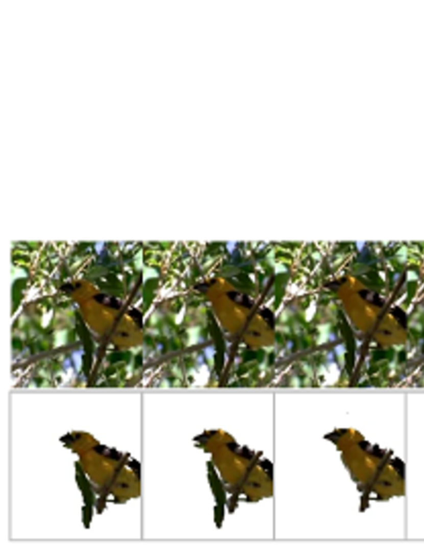
Figure 2: Example of a segmentation result (bottom) for some video (top) only with frame-wise saliency-based priors. We can see that segmented regions are frequently moved due to unstable behavior of visual saliency.

Although the above approaches are promising, they all pose a critical problem in that they have to provide segmentation cues (seeds) manually and carefully (See Figure 1). Such manual labeling is occasionally infeasible. The development of fully automatic segmentation methods has been strongly expected. Some previous work [9] utilized motion information to achieve fully automatic detection and segmentation of moving objects. However, targets we want to extract are not necessarily moving in video frames; target objects might be traffic signs, nameboards or statues that are all static. Also, a target object seems to be unmoving even though it is actually moving since a video camera can appropriately pursuit the target. Therefore, we need more versatile cues to extract various kinds of targets.

The use of saliency-based human visual attention models is one of the most promising approaches in this respect. The first biologically plausible model for explaining the human attention system was proposed by Koch and Ullman [10], and late implemented by Itti et al. [11]. This model analyzes still images to produce primary visual features (including intensity, color opponents, edge orientatiosn and motion information), which are combined to form a saliency map that represents the relevance of visual attention. Later, so many attempts have been made to improve the Koch-Ullman model [12, 13, 14, 15, 16] and to extend it to video signals [16, 17, 18, 19]. Our research group also proposed stochastic models [20, 21] for estimating human visual attention that tackled the fundamental problem of the previous attention models related to the non-deterministic properties of the human visual system. Such models would be helpful for automatically providing segmentation seeds.

To this end, we propose a novel approach for achieving video segmentation based on visual saliency. Our main contributions are as follows:

1) We newly incorporate saliency-based priors into frame-wise segmentation with graph cuts to achieve fully automatic segmentation. For the purpose of still image segmentation, this approach has been already appeared in the work undertaken by Fu et al. [5]. However, when dealing with video signals, segmentation results might be unstable (e.g. flickering or frequent moving) due to fluctuations of visual saliency. Figure 2 depicts a segmentation result with saliency-based priors derived from an input video. We can see from this figure that segmented regions are frequently moved due to the instability of visual saliency. We have to note that human visual attention might not be determined by only visual saliency representing a kind of novelty calcuated only from image signals; human visual attention is often controlled by their knowledge, experiences and intention. This is the reason why there is a discrepacy between highliy salient regions and intuitively attentive regions.

2) To tackle this problem, we develop a new technique for updating priors and feature likelihoods, which makes use of another property of the human visual system: temporal dependency of visual attention. We humans do not switch our attention to various regions so frequently, even though salient regions frequently move within a short period. Based on the above property, the new technique additionally introduces the segmentation result obtained from the previous frame to estimate a prior of the current frame. An idea of Kalman filter is utilized to integrate the previous segmentation result and saliency-based priors and to obtain the actual prior density for segmentation. Feature likelihoods can be also updated so as to reflect dominant feature components of the previous segmentation result. Nevertheless the above efforts, there still remains a crucial problem that it is still far from real-time processing due to its complex and costful procedures, especially in estimating saliency-based visual attention, calculating feature likelihoods, and deriving the segmentation results with graph cuts.

3) Thus, we introduce an implementation strategy making extensive use of stream processing with graphics processor units (GPUs) to accelerate the proposed method. Stream processing is not versatile for accelerating any kinds of signal processing: It is only feasible for computations that utilize simple data epeatedly and can compute each sub-process with almost the same calculation cost. We modify the algorithm so as to make it plausible for stream processing.

The rest of the paper is organized as follows: Section 2 describes the framework of the proposed method. Section 3 presents the procedure how to estimate human visual attention based on visual saliency. Section 4 explains a technique for supervised image segmentation based on graph cuts as a basis of our proposed method. Sections 5 to 7 present our main contributions of this paper, namely the method for providing saliency-based priors, the method for updating the priors according to the previous segmentation result, and their implementation based on the idea of stream processing. Section 8 discusses some quantitative evaluations. Finally, Section 9 summarizes the paper and discusses future work.

2 Framework

This section describes the framework of the proposed method for extracting salient regions from videos. Figure 3 depicts the framework.

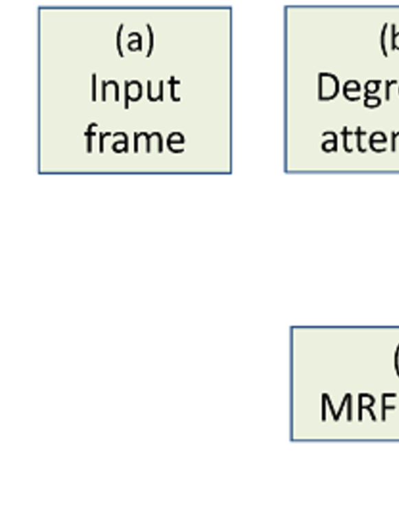
Figure 3: Framework of the proposed method

First, the visual attention density is calculated from each frame of an input video via a saliency-based human visual attention model. Although any kind of attention model can be employed, we utilize the model proposed by Pang et al. [20, 21] to compute the human visual attention density. Section 3 describes how to estimate human visual attention with the proposed method.

Next, a Markov random field (MRF) model for segmentation is prepared, where each hidden state corresponds to the label of a position representing an “object” or “background”, and an observation is a frame of the input frame. The density calculated in the previous step can be utilized for estimating the priors of objects/backgrounds and the feature likelihoods of the MRF. When calculating priors and likelihoods, the regions extracted from the previous frames are also available. Sections 5 and 6 focus particularly on how to determine and update priors and feature likelihoods based on the density of visual attention and previous segmentation results.

Once the MRF is constructed, salient regions can be obtained as the MAP solution of the MRF. When estimating the MAP solution, graph cuts based methods [2] can be employed. Section 4 presents the Interactive Graph Cuts method for image segmentation.

3 Estimation of human visual attention

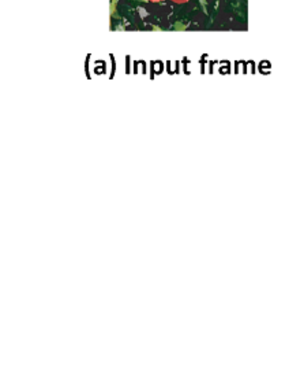
Figure 4: Eye-focusing density estimation through a stochastic model of human visual attention

Figure 4 shows the framework for estimating human visual attention. We used the stochastic model of human visual attention proposed by Pang et al. [20, 21].

First, a saliency map is calculated from each frame of the input video with the method proposed by Itti et al. [11]. Our implementation utilized intensity, color opponents, orientation and motion information as fundamental features.

Then, a stochastic representation of the saliency map is computed through a Kalman filter, where the saliency map is utilized as the observation of the filter. We call the stochastic representation of the saliency map as a stochastic saliency map. Each pixel of the stochastic saliency map is expressed by a Gaussian density.

The density of human visual attention can be directly calculated from the stochastic saliency map by introducing the principle of the signal detection theory [22], namely, the position at which stochastic saliency takes its maximum value is the eye focusing position. Since each pixel of the stochastic saliency map is expressed by a Gaussian, we can calculate the visual attention density for each pixel such that the saliency value has its maximum value at that pixel.

The model also incorporates another property, namely that eye movements may be affected by a cognitive state. The cognitive state is represented as an eye movement pattern in this model. Two typical eye movement patterns, passive and active, are found when a person is watching a video. By introducing the eye movement patterns, eye movements can be modeled with a hidden Markov model.

Finally, by integrating the density related to the bottom-up part (namely the stochastic saliency map) and the top-down part (namely the eye movement pattern), we can obtain the final density of visual attention, which is called the eye focusing density map (EFDM).

Although the above procedure well simulated the human visual system, it requires high computational costs (about 1 second per frame with a standard workstation). When considering this model as a pre-selection mechanism for subsequent processing (i.e. video segmentation), computational cost should be of crucial significance in terms of practical use. We have developed an algorithm plausible for stream processing [23], which incorporates a particle filter [24] with Markov chain Monte-Carlo sampling [25] into the basic model [20]. Details can be seen in [23, 26].

4 Segmentation with graph cuts

This section describes the supervised image segmentation technique based on graph cuts proposed by Boykov et al. [2].

We start by describing MRFs for image segmentation. Consider a set of random variables $\boldsymbol{A}=\{A_{\boldsymbol{x}}\}_{\boldsymbol{x}\in I}$ defined on a set $I$ of coordinates. Each random variable $A_{\boldsymbol{x}}$ takes a value $a_{\boldsymbol{x}}\in\{0,1\}$ corresponding to a background ($0$) and an object ($1$). Its inference can be formulated as an energy minimization problem where the energy corresponding to the configuration $\boldsymbol{A}$ is the negative log likelihood of the posterior density of the MRF, $E(\boldsymbol{A}|\boldsymbol{D})=-\log p(\boldsymbol{A}|\boldsymbol{D})$, where $\boldsymbol{D}$ represents the input image. The energy function consists of likelihood and prior terms defined as follows:

$$E(\boldsymbol{A}|\boldsymbol{D})=\sum_{\boldsymbol{x}\in I}\left\{\psi_{1}(\boldsymbol{D}|A_{\boldsymbol{x}})+\xi_{1}(A_{\boldsymbol{x}})\right.$$ (1)

$$+ \sum_{\boldsymbol{y}\in N_{\boldsymbol{x}}}\left(\psi_{2}(\boldsymbol{D}|A_{\boldsymbol{x}},A_{\boldsymbol{y}})+\xi_{2}(A_{\boldsymbol{x}},A_{\boldsymbol{y}})\right)\},$$

where $N_{\boldsymbol{x}}$ is a neighboring system for the position $\boldsymbol{x}$, $\psi_{i}(\boldsymbol{D}|\cdot)$ $(i=1,2)$ is a likelihood term and $\xi_{i}(\cdot)$ is a prior term. The first likelihood term $\psi_{1}(\boldsymbol{D}|A_{\boldsymbol{x}})$ imposes individual penalties for assigning label $a\in\{0,1\}$ to pixel $\boldsymbol{x}$, and it is given by $\psi_{1}(\boldsymbol{D}|A_{\boldsymbol{x}})=-\log p(C_{\boldsymbol{x}}|A_{\boldsymbol{x}})$, where $C_{\boldsymbol{x}}$ is the RGB value at the position $\boldsymbol{x}$. The likelihood $p(C_{\boldsymbol{x}}|A_{\boldsymbol{x}})$ of the RGB values can be modeled as a Gaussian mixture model (GMM), and estimated with a standard EM algorithm, where the number of Gaussians is given in advance as $M$. The first prior term $\xi_{1}(A_{\boldsymbol{x}})$ represents how the position is likely to a object, and can be determined by label manually given from users as

$$\xi_{1}(A_{\boldsymbol{x}}) = -\log p(A_{\boldsymbol{x}}),$$

$$p(A_{\boldsymbol{x}}=1) = \left\{\begin{array}[]{ll}1&\boldsymbol{x}\mbox{ has a manual label }1,\\ \epsilon\approx 0&\boldsymbol{x}\mbox{ has a manual label }0,\\ 0.5&\mbox{No label provided at }\boldsymbol{x}\end{array}\right.$$

$$p(A_{\boldsymbol{x}}=0) = 1-p(A_{\boldsymbol{x}}=1).$$

The second prior term $\xi_{2}(A_{\boldsymbol{x}},A_{\boldsymbol{y}})$ takes the form of a generalized Potts model as $\xi_{2}(A_{\boldsymbol{x}},A_{\boldsymbol{y}})=constant$ only if $A_{\boldsymbol{x}}\neq A_{\boldsymbol{y}}$. The second likelihood term $\psi_{2}(D|A_{\boldsymbol{x}},A_{\boldsymbol{y}})$ reduces the cost for two labels, which differs in proportion to the difference between the intensity values of their corresponding positions.

$$\psi_{2}(D|A_{\boldsymbol{x}},A_{\boldsymbol{y}}) \propto -\exp\left\{-\frac{(I_{\boldsymbol{x}}-I_{\boldsymbol{y}})^{2}}{2\sigma^{2}}\right\}\cdot\frac{1}{\|\boldsymbol{x}-\boldsymbol{y}\|}$$

$$\mbox{if }A_{\boldsymbol{x}}\neq A_{\boldsymbol{y}}$$

where $I_{\boldsymbol{x}}$ denotes the intensity at the pixel $\boldsymbol{x}$.

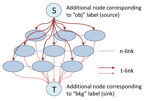
Figure 5: Graph for image segmentation

The MRF configuration $\widehat{\boldsymbol{a}}$ with the least energy corresponds to the MAP solution of the MRF. The energy minimization can be performed by finding the minimum cut on an equivalent graph of the MRF as shown in Figure 5. Each random variable $A_{\boldsymbol{x}}$ of the MRF is represented by a vertex $v_{\boldsymbol{x}}$ in this graph. A directed edge from each vertex $v_{\boldsymbol{x}}$ is connected to another vertex in its neighborhood $N_{\boldsymbol{x}}$. These edges are called as neighborhood links (n-links). The cost $c(v_{\boldsymbol{x}},v_{\boldsymbol{y}})$ associated with the n-link $(\boldsymbol{x},\boldsymbol{y})$ connecting from $v_{\boldsymbol{x}}$ to $v_{\boldsymbol{y}}$ is given by the sum of the second prior and likelihood terms as

$$c(v_{\mbox{\boldmath$x$}},v_{\mbox{\boldmath$y$}}) = \psi_{2}(D|A_{\mbox{\boldmath$x$}},A_{\mbox{\boldmath$y$}})+\xi_{2}(A_{\mbox{\boldmath$x$}},A_{\mbox{\boldmath$y$}}).$$ (3)

Also, the graph has two special vertices the source $s$ and the sink $t$ each of which corresponds to the label $0$ and $1$. Directed edges called terminal links (t-links) are connected from the source to all the other vertices except the sink and from all the vertices except the source to the sink. The costs $c(s,\boldsymbol{vv}_{\boldsymbol{x}})$ and $c(t,\boldsymbol{vv}_{\boldsymbol{x}})$ of t-links are given by the sum of the first prior and likelihood terms as

$$c(s,v_{\mbox{\boldmath$x$}}) = \psi_{1}(D|A_{\mbox{\boldmath$x$}}=0)+\xi_{1}(A_{\mbox{\boldmath$x$}}=0),$$ (4)

$$c(v_{\mbox{\boldmath$x$}},t) = \psi_{1}(D|A_{\mbox{\boldmath$x$}}=1)+\xi_{1}(A_{\mbox{\boldmath$x$}}=1).$$ (5)

The minimum cut of the graph separating the source and the sink provides the MAP configuration $\widehat{\boldsymbol{a}}$ of the corresponding MRF.

5 Saliency-based priors

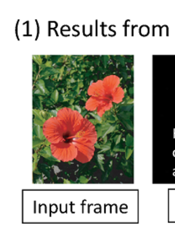
Figure 6: Saliency-based priors

As the first contribution of this paper, we provide a way to calculate the first prior term of the energy function shown in Equation (1) without any manually provided labels. We utilize the density of visual attention calculated by the procedure shown in Section 3. Figure 6 shows a sketch for calculating the prior.

The prior density $p(A_{\boldsymbol{x}}=1)$ is obtained from the EFDM (cf. Section 3). We represent the EFDM with a Gaussian mixture model (GMM), and estimate the model parameter with the EM algorithm. The estimated GMM density represents the prior density $p(A_{\boldsymbol{x}}=1)$. Exceptionally, the prior on the edge of each frame is assumed to be $p(A_{\boldsymbol{x}}=1)\approx 0$ since some of the background regions are expected to be at the frame edge.

The likelihood density $p(C_{\boldsymbol{x}}|A_{\boldsymbol{x}})$ can be obtained in the same way as the Interactive Graph Cuts [2]. Although in the Interactive Graph Cuts, samples are selected from the manually-labeled pixels for estimating the likelihood density $p(C_{\boldsymbol{x}}|A_{\boldsymbol{x}})$, our proposed method utilizes all the pixels, where samples are weighted by the prior density $p(A_{\boldsymbol{x}}=1)$.

6 Prior update

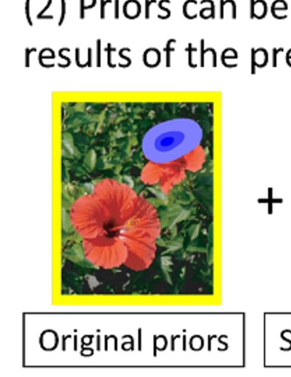
Figure 7: Prior update

The second contribution provided by our method is that it offers a way to update the prior and likelihood terms according to the segmentation results derived from the previous frames and the density of visual attention calculated from the current frame. Figure 7 shows a sketch for prior update. Here, we introduce a notation $\boldsymbol{A}_{t}=\{A_{\boldsymbol{x},t}\}_{\boldsymbol{x}\in I}$ $(t=0,1,\cdots)$ for representing the MRF configuration at time $t$.

To update the prior density $p(A_{\boldsymbol{x},t})$ at time $t$, we introduce an idea of Kalman filter [24], where the prior density derived solely from the EFDM at time $t$ (from now on, we denote it as $q(A_{\boldsymbol{x},t})$) is considered to be the observation at time $t$. We assume the following two relationships:

$$p(A_{\boldsymbol{x},t}=1) = f(\widehat{\boldsymbol{A}}_{t-1},\boldsymbol{x})+N_{1},$$

$$q(A_{\boldsymbol{x},t}=1) = p(A_{\boldsymbol{x},t}=1)+N_{2},$$

where $\widehat{\boldsymbol{A}}_{t}$ is the estimated MRF configuration at time $t$, $N_{i}$ $(i=1,2)$ is a Gaussian random variable with mean $0$ and variance $\sigma^{2}_{i}$, and $f(\boldsymbol{A},\boldsymbol{x})$ represents a pixel value at $\boldsymbol{x}$ of a gray-scaled image obtained from an MRF configuration $\boldsymbol{A}$ with some image processing e.g. Gaussian smoothing [4] or distance transform [6]. These equations imply that the prior density at the current frame depends on both the EFDM at the current frame and the segmentation result of the previous frame.

The estimate $\widehat{p}(A_{\boldsymbol{x},t}=1)$ of the prior density at time $t$ can be derived as

$$\widehat{p}(A_{\mbox{\boldmath$x$},t}=1) = \frac{\sigma^{2}_{1}}{\sigma^{2}_{1}+\sigma^{2}_{2}+\sigma^{2}_{\xi_{1}}(t-1)}f(\mbox{\boldmath$\widehat{A}$}_{t-1},\mbox{\boldmath$x$})$$

$$+ \frac{\sigma^{2}_{2}+\sigma^{2}_{\xi_{1}}(t-1)}{\sigma^{2}_{1}+\sigma^{2}_{2}+\sigma^{2}_{\xi_{1}}(t-1)}q(A_{\mbox{\boldmath$x$},t}=1),$$

$$\sigma^{2}_{\xi_{1}}(t) = \frac{\sigma^{2}_{1}\cdot(\sigma^{2}_{2}+\sigma^{2}_{\xi_{1}}(t-1))}{\sigma^{2}_{1}+\sigma^{2}_{2}+\sigma^{2}_{\xi_{1}}(t-1)}.$$

The estimate $\widehat{p}(A_{\boldsymbol{x},t}=1)$ derived from the above procedure is used as a new prior density.

7 GPU implementation

7.1 Stream processing

In recent years, there has been strong interest from researchers and developers in exploiting the power of commodity hardware including multiple processor cores for parallel computing. This is because 1) multi-core CPUs and stream processors such as graphics processing units (GPUs) and Cell processors [27] are currently the most powerful and economical computational hardware available, 2) the rise of SDKs and APIs such as NVIDIA CUDA [28], AMD ATiStream [29], OpenCL [30] and Microsoft DirectCompute [31] makes it easy to implement desired algorithms for execution on multi-core hardware. This programming paradigm is widely known as stream processing. However, stream processing is not versatile for accelerating any kinds of signal processing: Stream processing is only feasible for computations that utilize simple data repeatedly and can compute each sub-process with almost the same calculation cost. When we make extensive use of stream processing, we have to modify the algorithm to fit the above property.

We are focusing on GPUs as prospective hardware for stream processing, due to its powerful performance and availability. Previously, we needed to master shader programming languages such as HLSL [31] and GLSL [30] as well as to understand graphics pipelines for the extensive use of GPUs. NVIDIA CUDA [28] makes it easy to implement a wide variety of (numerical, now always graphics-related) algorithms without any special knowledge and artifices. Its interface is quite similar to C, and its function can be called in standard C/C++ platforms.

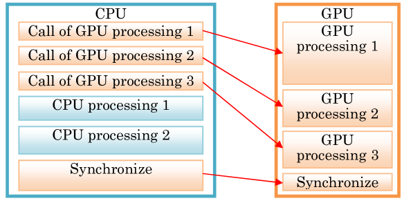
Figure 8: Asynchronous execution of CPU and GPU processing

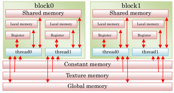
Figure 9: Memory model on CUDA

TABLE I: Characteristics of physical memories on GPU

Type	Read	Write	Data	Cache	Synchro-
			transfer		nization
Global	OK	OK	OK	NG	Grids
Texture	OK	NG	OK	OK	—
Constant	OK	NG	OK	OK	—
Shared	OK	OK	NG	—	Blocks
Local	OK	OK	NG	—	—
Register	OK	OK	NG	—	—

Although CUDA enables us to implement various kinds of algorithms easier than before, we should still take care of its programming model and memory model for the extensive use. As shown in Figure 8, once GPU processing is called from a CPU functions, it is queued in line by a graphics driver and executed sequentially and asynchronously. This implies that excess computational resources of CPU can be assigned to other computations such as data transfer between CPU and GPU. Also, as shown in Figure 9 and Table I, CUDA can handle 6 different types of memories: Global, texture, constant, shared, local and register. Moreover, data transfer between CPU and GPU often becomes the bottle neck for the acceleration. From the above discussion, we have to carefully consider the order and timing of function calls for GPU, and select the type of memories according to the usage.

7.2 Visual attention estimation

Almost all the parts for estimating visual attention have been already implemented on GPU, however, saliency map calculation [11] still remains as a CPU processing. This section details how to implement saliency map calculation on GPU.

Saliency map calculation consists of 1) fundamental feature extraction such as intensity, color opponents, edge orientation and optical flow, 2) Gaussian pyramid construction, 3) a special normalization function utilizing the global and local minimum of pixel values, and 4) weighted addition of images. These computation can be roughly classified into the following 3 types: pixel-wise computation, filter convolution, and local extrema detection. In the following, we detail each procedure of.

⬇

1texture<float, 1, cudaReadModeElementType> filter;

2texture<float, 1, cudaReadModeElementType> src1;

3__device__ float Filter2DCore(texture<float, 1, cudaReadModeElementType> fsource, int x, int y, int height, int width, int filterSizeX, int filterSizeY) {

4 float sum = 0;

5 x -= filterSizeX/2;

6 y -= filterSizeY/2;

7 for(int fy = 0; fy < filterSizeY; fy++) {

8 int by = y + fy;

9 if(by > 0 && by < height) {

10 by *= width;

11 for(int fx = 0; fx < filterSizeX; fx++) {

12 int bx = x + fx;

13 if(bx > 0 && bx < width) {

14 sum += tex1Dfetch(filter, fy*filterSizeX + fx)*tex1Dfetch(fsource, by + bx);

15 }

16 }

17 }

18 }

19 return sum;

20}

21__global__ void Filter2DKernel(int height, int width, int fheight, int fwidth, float* result) {

22 int px = blockDim.x*blockIdx.x + threadIdx.x;

23 if(px < height*width) {

24 int x = px%width;

25 int y = px/width;

26 result[px] = Filter2DCore(src1, x, y, height, width, fwidth, fheight);

27 }

28}

Figure 10: CUDA implementation for filtering

A pixel value $F(\boldsymbol{x})$ of the filtered image at the position $\boldsymbol{x}$ can be derived by convoluting the original image $\boldsymbol{D}$ with a filter kernel $F_{k}(\boldsymbol{x})$ with size $n\times m$ as follows:

$$F(x,y) = \sum_{i=0}^{n}\sum_{j=0}^{m}F_{k}(i,j)$$

$$*P\left(x+i-\frac{n}{2},y+j-\frac{m}{2}\right).$$

The image $P(x,y)$ and filter kernel $F_{k}(i,j)$ are transferred to and placed on the texture memory, and the filter output $F(x,y)$ is set on the global memory. This allocation would enhance the performance of memory access since the filter kernel $F_{k}(i,j)$ are utilized by every kernel and every pixel $P(x,y)$ of the image is accessed by several threads. A pseudo code for filter convolution is shown in Figure 10.

Gaussian pyramids can be efficiently constructed by setting the image on the texture memory.

⬇

1texture<float, 1, cudaReadModeElementType> minsrc;

2texture<float, 1, cudaReadModeElementType> maxsrc;

3__global__ void SMRangeNormalizeKernel1(int length, float* localmin, float* localmax) {

4 int px = blockDim.x*blockIdx.x + threadIdx.x;

5

6 __shared__ float mini[32], maxi[32];

7 if(px < length) {

8 mini[threadIdx.x] = tex1Dfetch(minsrc, px);

9 maxi[threadIdx.x] = tex1Dfetch(maxsrc, px);

10 } else {

11 mini[threadIdx.x] = FLT_MAX;

12 maxi[threadIdx.x] = FLT_MIN;

13 }

14 __syncthreads();

15 if(threadIdx.x == 0) {

16 for(int i = 1; i < blockDim.x; i++) {

17 mini[0] = min(mini[0], mini[i]);

18 maxi[0] = max(maxi[0], maxi[i]);

19 }

20 localmin[blockIdx.x] = mini[0];

21 localmax[blockIdx.x] = maxi[0];

22 }

23}

Figure 11: Minimum/maximum search

Figure 11 shows a pseudo code for searching the global and local extrema of pixel values in the image, where a buffer for the minima (resp. maxima) is denoted as minsrc (resp. maxsrc). Every pixel value in a block is first obtained and stored in the shared memory. Then, all the thread in the block are synchronized by calling the function __syncthreads, and some specific thread (e.g. thread 0) computes the maximum and minimum in the block. As a result, a smaller image having the same number of pixels as the number of blocks and pixel values of the minimum (resp. minimum) of every blocks is generated. This procedure is repeatedly executed until the number of pixels converges.

7.3 Segmentation

For the segmentation procedure, we newly implement the algorithm for deriving priors, feature likelihoods and minimum cuts on GPU.

Priors can be calculated in almost the same way as described in the previous section, since the procedure is composed of Gaussian filtering and pixel-wise Kalman filter.

For the derivation of t-link costs, we first estimate GMM model parameters of RGB values (see Section 4) with EM algorithm, which has been already implemented and distributed by Harp [32]. We utilized k-means algorithm implemented on CPU for the initialization of the EM algorithm. T-link costs are the negative log likelihood of image features, which can be implemented on GPU by a combination of Gaussian filtering. Only the normalization term of each Gaussian density is calculated on CPU.

For the graph cuts, we can find several implementations with CUDA. We utilized CUDA Cuts [33] developed by Vineet et al.

8 Experiments

8.1 Conditions

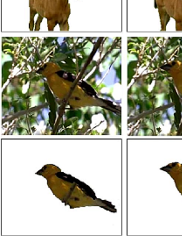
Figure 12: Samples of input videos and corresponding ground truth made by hands

To verify the effectiveness of the proposed method, we conducted video segmentation for 10 video clips of length 5-10 seconds and 12 fps. For each video, we have made ground-truth segmented video frames by hands. Some examples can be seen in Figure 12. As a measure for quantitative evaluation, we adopted error rate, precision, recall and F-value defined as follows:

$${\rm Error} = \frac{FP+FN}{TP+TN+FP+FN},$$

$${\rm Recall} = \frac{TP}{TP+FN},$$

$${\rm Precision} = \frac{TP}{TP+FP},$$

$${\rm F-value} = \frac{2\times{\rm Recall}\times{\rm Precision}}{{\rm Recall}+{\rm Precision}},$$

where TP, TN, FP and FN respectively represents the number of true positives, true negatives, false positives and false negatives. We compared our new method with the following methods

1. Manual: Manually-provided labels were available for the segmentation only in the first frame. For the other frames, priors and feature likelihoods were estimated from the previous segmentation result. This strategy is quite similar to the semi-automatic method developed by Kohli and Torr [8].

2. Non-update: Only saliency-based priors were available and any previous segmentation results cannot be utilized for the segmentation. This strategy simulates the fully automatic method developed for still images by Fu et al. [5].

3. Update: Our proposed method

TABLE II: Platform used in the evaluation

CPU	Intel Core2Quad Q9550
Memory	4GB
GPU	NVIDIA Geforce 9800GT
Graphics memory	512MB
OS	Windows XP Professional
Software	NVIDIA CUDA 2.1
	OpenCV 1.1pre

We experimentally determined parameters in advance as follows: $\sigma_{1}=0.03,\sigma_{2}=0.035,M=3$. The platform used in the evaluation is shown in Table II.

8.2 Segmentation accuracy

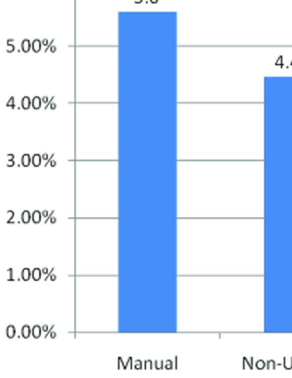
Figure 13: Evaluation result measured by the error rate

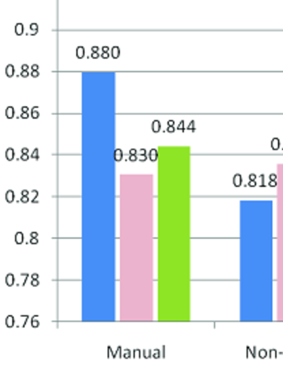
Figure 14: Evaluation result measured by recall, precision and F-measure

Figure 13 shows the segmentation accuracy measured by the error rate, and Figure 14 shows the accuracy measured by precision, recall and F-measure. These results indicates that our proposed method outperformed the other methods under all the conditions.

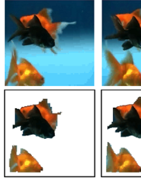
Figure 15: Segmentation examples emitted from the proposed method

Figure 15 shows some examples emitted from our proposed method. By comparing it with Figure 12, we can see that our proposed method worked well from the qualitative aspect.

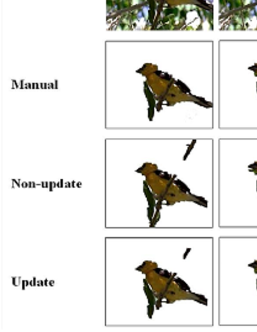
Figure 16: Comparing segmentation results emitted from all the 3 methods

Figure 16 shows an example of segmentation results emitted from all the methods used in this evaluation. The method “manual” could not recover from incorrect segmentation once the target (in this case a bird) lost, since this method only utilized the previous segmentation results as a cue for detecting the target. This indicates the advantages of saliency-based priors. The segmentation results emitted from the method “non-update” sometimes became unstable due to some noises or fluctuations included in saliency information. This implies that temporal smoothness by utilizing the previous segmentation result is also significant for stable segmentation.

TABLE III: Comparing error rates [%]

	Boykov [1]	Nagahashi [4]	Proposed
Error	3.75	1.61	2.74

TABLE IV: Comparing recall, precision and F-measure

	Boykov [2]	Nagahashi [7]	Proposed
Recall	0.88	0.91	0.895
Precision	0.96	0.88	0.858
F-value	0.92	0.89	0.866

We show some reference information as to the segmentation accuracy. Table III presents error rates published in the papers of Boykov et al. [1] and Nagahashi et al. [4], both of which are specialized for still image segmentation with manually provided labels. Table IV shows precision, recall and F-measure published in the paper of Boykov et al. [2] and Nagahashi et al. [7], both of which are specialized for video segmentation with manually provided labels. This table indicates that our proposed method marked high segmentation accuracy comparable with the previously proposed semi-automatic segmentation methods. Note that videos used for the evaluation differs from each other.

8.3 Execution time

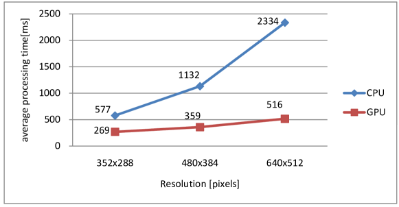
Figure 17: Average execution time per frame

TABLE V: Detailed execution time per frame [ms]

		VA	Priors	t-link	Graph	Misc
					cuts
352	CPU	32.9	148.1	218.6	97.0	71.0
$\times$288	GPU	22.2	1.9	109.6	69.0	65.6
480	CPU	58.8	372.8	350.8	246.5	86.4
$\times$384	GPU	30.4	3.5	120.8	27.7	74.6
640	CPU	109.8	814.5	602.6	664.5	112.7
$\times$512	GPU	45.2	6.2	142.6	232.3	87.1

Figure 17 shows the average execution time per frame for the cases of CPU and GPU implementations, and Table V shows the detailed execution time per frame for each step, where “misc” includes the time for capturing video frames, memory allocation and release. These results indicate that GPU implementation greatly improve the execution time, e.g. 132 times in deriving saliency-based priors and 4.5 times in total than the CPU implementation. These results also indicates that as the video resolution increased the execution time per pixel decreased in the GPU implementation, while the opposite in the CPU implementation.

TABLE VI: Comparison of execution time with previous methods

[1]	[4]	[2]	[7]	Proposed
300$\times$255	300$\times$255	360$\times$240	360$\times$240	352$\times$288
0.94	37.59	329.6	181.6	0.294

We show some reference information also as to the execution time. Table VI presents the execution time published in the papers of Boykov et al. [1, 2] and Nagahashi et al. [4, 7]. This table indicates that our proposed method finished all the procedures much faster than others. Again note that videos used for the evaluation differs from each other.

9 Conclusion

We have proposed a new and quite fast method for automatic video segmentation with the help of 1) efficient optimization of Markov random fields with polynomial time of number of pixels by introducing graph cuts, 2) automatic, computationally efficient but stable derivation of segmentation priors using visual saliency and sequential update mechanism, and 3) an implementation strategy in the principle of stream processing with graphics processor units (GPUs). Experimental results indicated that our method extracted appropriate regions from videos as precisely as and much faster than previous semi-automatic methods even though any supervisions have not been incorporated. Future work includes development of more sophisticated segmentation methods utilizing such as top-down information or text information.

References

- [1] Boykov, Y. and Jolly, M. (2004) Interactive graph cuts for optimal boundary and region segmentation of objects in N-D images. Proc. Conference on Computer Vision and Pattern Recognition (CVPR), pp. 731–738.
- [2] Boykov, Y. and Lea, G. (2006) Graph cuts and efficient N-D image segmentation. International Journal of Computer Vision, 70, 109–131.
- [3] Greig, D., Porteous, B., and Seheuit, A. (1989) Exact maximum a posteriori estimation for binary images. Royalstat, B:51, 271–279.
- [4] Nagahashi, T., Fujiyoshi, H., and Kanade, T. (2007) Image segmentation using iterated graph cuts based on multi-scale smoothing. Proc. Asian Conference on Computer Vision (ACCV), pp. pp. 806–816.
- [5] Fu, Y., Cheng, J., Li, Z., and Lu, H. (2008) Saliency cuts: An automatic approach to object segmentation. Proc. International Conference on Pattern Recognition (ICPR).
- [6] Fukuda, K., Takiguchi, T., and Ariki, Y. (2008) Graph cuts by using local texture features of wavelet coefficient for image segmentation. Proc. International Conference on Multimedia and Expo (ICME), pp. 881–884.
- [7] Nagahashi, T., Fujiyoshi, H., and Kanade, T. (2009) Video segmentation using iterated graph cuts based on spatio-temporal volumes. Proc. Asian Conference on Computer Vision (ACCV).
- [8] Kohli, P. and Torr, P. (2007) Dynamic graph cuts for efficient inference in markov random fields. IEEE Transactions on Pattern Analysis and Machine Intelligence, 29, 2079–2088.
- [9] Liu, F., and Gleicher M. (2009) Learning color and locality cues for moving object detection and segmentation. Proc. IEEE International Conference on Computer Vision and Pattern Recognition (CVPR).
- [10] Koch, C. and Ullman, S. (1985) Shifts in selective visual attention: Towards the underlying neural circuitry. Human Neurobiology, 4, 219–227.
- [11] Itti, L., Koch, C., and Niebur, E. (1998) A model of saliency-based visual attention for rapid scene analysis. IEEE Transactions on Pattern Analysis and Machine Intelligence, 20, 1254–1259.
- [12] Privitera, C. M. and Stark, L. W. (2000) Algorithms for defining visual regions-of-interest: Comparison with eye fixations. IEEE Transactions on Pattern Analysis and Machine Intelligence, 22, 970–982.
- [13] Gu, E., Wang, J., and Badler, N. (2005) Generating sequence of eye fixations using decision-theoretic attention model. Proc. Conference on Computer Vision and Pattern Recognition (CVPR), June, pp. 92–99.
- [14] Frintrop, S. (2006) Vocus: a Visual Attention System for Object Detection And Goal-directed Search (Lecture Notes in Computer Science). Springer-Verlag New York Inc (C).
- [15] Jeong, S., Ban, S., and Lee, M. (2008) Stereo saliency map considering affective factors and selective motion analysis in a dynamic environment. Neural Networks, 21, 1420–1430.
- [16] Gao, D. and Vasconcelos, N. (2009) Decision-theoretic saliency: Computational principles, biological plausibility, and implications for neurophysiology and psychophysics. Neural Computation, 21, 239–271.
- [17] Itti, L. and Baldi, P. (2005) A principled approach to detecting surprising events in video. Proc. Conference on Computer Vision and Pattern Recognition (CVPR), June, pp. 631–637.
- [18] Leung, C., Kimura, A., Takeuchi, T., and Kashino, K. (2007) A computational model of saliency depletion/recovery phenomena for the salient region extraction of videos. Proc. International Conference on Multimedia and Expo (ICME), July, pp. 300–303.
- [19] Ban, S., Lee, I., and Lee, M. (2007) Dynamic visual selective attention model. Neurocomputing, 71, 853–856.
- [20] Pang, D., Kimura, A., Takeuchi, T., Yamato, J., and Kashino, K. (2008) A stochastic model of selective visual attention with a dynamic Bayesian network. Proc. International Conference on Multimedia and Expo (ICME), June, pp. 1076–1079.
- [21] Kimura, A., Pang, D., Takeuchi, T., Yamato, J., and Kashino, K. (2008) Dynamic Markov random field for stochastic modeling of visual attention. Proc. International Conference on Pattern Recognition (ICPR), December Mo.BT8.35.
- [22] Eckstein, M. P., Thomas, J. P., Palmer, J., and Shimozaki, S. S. (2000) A signal detection model predicts effects of set size on visual search accuracy for feature, conjunction, triple conjunction and disjunction displays. Perception and Psychophysics, 62, 425–451.
- [23] Miyazato, K., Kimura, A., Takagi, S., and Yamato, J. (2009) Real-time estimation of human visual attention with mcmc-based particle filter. Proc. International Conference on Multimedia and Expo (ICME), June.
- [24] Ristic, B., Arulampalam, S., and Gordon, N. (2004) Beyond the Kalman filter: Particle filters for tracking applications. Artech House Publishers, Boston.
- [25] Andrieu, C., Defreitas, N., Doucet, A., and Jordan, M. (2003) An introduction to mcmc for machine learning. Machine Learning, 50, 5–43.
- [26] Kimura, A., Pang, D., Takeuchi, T., Miyazato, K., Yamato, J., and Kashino, K. (2010) A stochastic model of selective visual attention with a dynamic Bayesian network. IEEE Transactions on Pattern Analysis and Machine Intelligence , ? submitted.
- [27] Mallinson, D. and DeLoura, M. (2005) CELL: A new platform for digital entertainment. Game Developers Conference, March.
- [28] NVIDIA Corporation (2008) CUDA programming guide Ver.2.0. http://www.nvidia.co.jp/object/cuda\_home\_jp.html.
- [29] http://www.amd.com/us/products/technologies/stream-technology/Pages/strea%m-technology.aspx.
- [30] http://www.khronos.org/opencl/.
- [31] http://msdn.microsoft.com/en-us/library/ee663301(VS.85).aspx.
- [32] Harp, A. Computational statistics via GPU. http://andrewharp.com/gmmcuda.
- [33] Vineet, V. and Narayanan, P. J. (2008) Cuda cuts: Fast graph cuts on the gpu. CVPR Workshop on Visual Computer Vision on GPUs.