Research Announcement: Finite–time Blow Up and Long–wave Unstable Thin Film Equations

Abstract

We study short–time existence, long–time existence, finite speed of propagation, and finite–time blow–up of nonnegative solutions for long-wave unstable thin film equations $h_{t}=-a_{0}(h^{n}h_{xxx})_{x}-a_{1}(h^{m}h_{x})_{x}$ with $n>0$, $a_{0}>0$, and $a_{1}>0$. The existence and finite speed of propagation results extend those of [Comm Pure Appl Math 51:625–661, 1998]. For $0<n<2$ we prove the existence of a nonnegative, compactly–supported, strong solution on the line that blows up in finite time. The construction requires that the initial data be nonnegative, compactly supported in $\mathbb{R}^{1}$, be in $H^{1}(\mathbb{R}^{1})$, and have negative energy. The blow-up is proven for a large range of $(n,m)$ exponents and extends the results of [Indiana Univ Math J 49:1323–1366, 2000].

2000 MSC: 35K65, 35K35, 35Q35, 35B05, 35B45, 35G25, 35D05, 35D10, 76A20

keywords: fourth-order degenerate parabolic equations, thin liquid films, long–wave unstable, finite–time blow–up, finite speed of propagation

1 Introduction

Numerous articles have been published since the early sixties concerning the problem of developing finite-time singularities by solutions of nonlinear parabolic equations (see the survey papers of Levine [31] and of Bandle and Brunner [2]). Such problems arise in various applied fields such as combustion theory, the theory of phase separation in binary alloys, population dynamics and incompressible fluid flow.

Whether or not there is a finite–time singularity, such as $\|u(\cdot,t)\|_{\infty}\to\infty$ as $t\to T^{*}<\infty$, is strongly affected by the nonlinearity in the PDE. For example, consider the semilinear heat equation on the line:

$$u_{t}=u_{xx}+u^{p},$$ (1.1)

where $u$ is real–valued. If $p\leqslant 1$ then a solution of an initial value problem exists for all time. If $1<p\leqslant 3$, then any non-trivial solution blows up in finite time. If $p>3$ then some initial data yield solutions that exist for all time and other initial data result in solutions that have finite–time singularities. The manner in which solutions blow up is well understood computationally and analytically. The blow up is of a focussing type: there are isolated points in space around which the graph of the solution narrows and becomes taller as $t\uparrow T^{*}$, converging to delta functions centered at the blow–up points. As $t\uparrow T^{*}$, the behaviour of the solution near the blow–up point(s) becomes more and more self–similar. Proving this convergence to a self–similar solution uses the maximum principle, which doesn’t hold for fourth–order equations like the one we study in this article.

We study the longwave-unstable generalized thin film equation,

$$h_{t}=-a_{0}\,(|h|^{n}\,h_{xxx})_{x}-a_{1}\,(|h|^{m}\,h_{x})_{x},$$ (1.2)

where $a_{0}>0$, $a_{1}>0$, and $h$ is real valued. Perturbing a constant steady state slightly, $h_{0}(x)=\bar{h}+\epsilon h_{1}(x,0)=\bar{h}+\epsilon\cos(\xi x+\phi)$, and linearizing the equation about $\bar{h}$, the small perturbation $h_{1}(x,t)$ will (approximately) satisfy $h_{t}=-a_{0}|\bar{h}|^{n}h_{xxxx}-a_{1}|\bar{h}|^{m}h_{xx}$. Hence the constant steady state is linearly unstable to long wave perturbations:

$$\xi^{2}<|\bar{h}|^{m-n}a_{1}/a_{0}\quad\Longrightarrow\quad h_{1}(x,t)\sim e^{-a_{0}\xi^{2}|\bar{h}|^{n}\left(\xi^{2}-\tfrac{a_{1}}{a_{0}}|\bar{h}|^{m-n}\right)t}\cos(\xi x+\phi)\quad\mbox{grows}.$$ (1.3)

Such equations arise in the modelling of fluids and materials. For example, equation (1.2) with $n=m=1$ describes a thin jet in a Hele-Shaw cell [16] where $h$ represents the thickness of the jet and $x$ is the axial direction; if $n=3$ and $m=-1$ equation (1.2) describes Van der Waals driven rupture of thin films [44] where $h$ represents the thickness of the film; if $n=m=3$ the equation models fluid droplets hanging from a ceiling [21] with $h$ representing the thickness of the film, and finally if $n=0$ and $m=1$ the equation is a modified Kuramoto-Sivashinsky equation and describes the solidification of a hyper-cooled melt [9] where $h$ desribes the deviation from flatness of a near planar interface. We note that in the first three cases the solution $h$ must be nonnegative for the model to make physical sense.

Hocherman and Rosenau [28] considered whether or not equation (1.2) could have solutions that blow up in finite time. They conjectured that if $n>m$ then solutions might blow up in finite time but if $n<m$ they would exist for all time. Indeed, this conjecture is natural if one considers the linear stability of a constant steady state $\bar{h}$: if $n>m$ the unstable band (1.3) grows as $\bar{h}\to\infty$ suggesting that $n=m$ is critical.

Hocherman and Rosenau considered general, real–valued solutions. However, if $n>0$ equation (1.2) may have solutions that are nonnegative for all time. Bertozzi and Pugh [12] proposed that if the boundary conditions are such that the mass, $\int h(x,t)\;dx$, is conserved then mass conservation, combined with the nonnegativity results in a different balance: $m=n+2$ instead of $m=n$. For such cases they introduced the regimes

$$\begin{cases}m<n+2\Longrightarrow\mbox{subcritical regime}\\ m=n+2\Longrightarrow\mbox{critical regime}\\ m>n+2\Longrightarrow\mbox{supercritical regime}\end{cases}$$

In [12], Bertozzi and Pugh considered equation (1.2) on a finite interval with periodic boundary conditions. For a subset of the subcritical ($m<n+2$) regime they proved some global-in-time results. Specifically, they proved that given positive initial data, $h_{0}>0$, there is a nonnegative weak solution of (1.2) that exists for all time if $0<n\leqslant m<n+2$. By restricting $n$ further to $0<n<3$ they can consider nonnegative initial data, $h_{0}\geqslant 0$. They prove that there a nonnegative weak solution that exists for all time and also prove the local entropy bound needed for the finite speed of propagation proof for $0<n<2$. For the critical ($m=n+2$) regime, they prove that the above results will hold if the mass $\int h_{0}\;dx$ is sufficiently small. Also, they provided numerical simulations suggesting that other initial data can result in solutions that blow up in finite time and conjectured that this is also true for the supercritical ($m>n+2$) regime.

In [13], they considered equation (1.2) on the line and found some analytical results for the critical and supercritical ($m\geqslant n+2$) regimes in the special case of $n=1$. They introduced a large class of ‘‘negative energy’’ initial data and proved that given initial data $h_{0}$ with compact support and negative energy there is a nonnegative weak solution $h$ that blows up in finite time: there is a time $T^{*}<\infty$ such that the weak solution $h(\cdot,t)$ exists on $[0,T^{*})$ and

$$\limsup_{t\to T^{*}}\|h(\cdot,t)\|_{L^{\infty}}=\infty\qquad\mbox{and}\qquad\limsup_{t\to T^{*}}\|h(\cdot,t)\|_{H^{1}}=\infty.$$

The blow–up time $T^{*}$ depends only on $m$ and $H^{1}$-norm of the initial data. We note that uniqueness of nonnegative weak solutions of (1.2) is an open problem. Indeed, there are simple counterexamples to uniqueness for the simplest equation $h_{t}=-(h^{n}h_{xxx})_{x}$ (see, e.g. [4]) although it is hypothesized that solutions are unique if one considers the question within a sufficiently restrictive class of weak solutions. For this reason, one cannot exclude the possibility that the initial data $h_{0}$ might also be achieved by a different weak solution, one that exists for all time.

Their proof relied on a second moment argument, found formally by Bernoff [8]: if $h$ is a smooth compactly-supported solution of (1.2) on $[0,T^{*})$ then the second moment of $h$ satisfies

$$\int\limits_{-\infty}^{\infty}x^{2}h(x,t)\;dx\leqslant\int\limits_{-\infty}^{\infty}x^{2}h_{0}(x)\;dx+6\mathcal{E}(0)\,t$$ (1.4)

holds for all $t\in[0,T^{*})$. Here, $\mathcal{E}(0)$ is the energy of the initial data:

$$\mathcal{E}(0):=\int\limits_{-\infty}^{\infty}\left\{\tfrac{a_{0}}{2}{h_{0}}_{x}^{2}(x)-\tfrac{a_{1}}{m(m+1)}h_{0}^{m+1}(x)\right\}\;dx.$$ (1.5)

As a result, there could never be a global-in-time nonnegative smooth solution with negative-energy initial data: for such a solution the left–hand side of (1.4) would always be nonnegative but the right–hand side would become negative in finite time. (This argument is strictly formal because, to date, no-one has constructed nonnegative, compactly-supported, smooth solutions on the line.) The blow-up result is found by first proving the short-time existence of a nonnegative, compactly-supported, weak solution: it exists on $[0,T_{0}]$ where the larger $\|h_{0}\|_{H^{1}}$ is, the smaller $T_{0}$ will be. Also, the constructed solution satisfies the second moment inequality (1.4) at time $t=T_{0}$. By ‘‘time–stepping’’ the short-time existence result, they construct a solution on $[0,T^{*})$ such that the second moment inequality (1.4) holds at a sequence of times $T_{i}$ with $T_{i}\to T^{*}$. It then follows immediately that $T^{*}$ must be finite and therefore the $\limsup_{t\to T^{*}}\|h(\cdot,t)\|_{H^{1}}$ must be infinite.

Outline of results

The main results of this paper are: short-time existence of nonnegative strong solutions on $[-a,a]$ given nonnegative initial data, finite speed of propagation for these solutions if their initial data had compact support within $(-a,a)$, and finite-time blow-up for solutions of the Cauchy problem that have initial data with negative energy.

First, we consider equation (1.2) on a bounded interval $[-a,a]$ with periodic boundary conditions. Given nonnegative initial data that has finite ‘‘entropy’’, in Theorem 1 we prove the short-time existence of a nonnegative weak solution if $n>0$ and $m\geqslant n/2$. The solution is a ‘‘generalized weak solution’’ as described in Section 2 and the entropy is introduced in Section 3. Additional regularity is proven in Theorem 2: there is a second type of entropy such that if this ‘‘$\alpha$-entropy’’ is also finite for the initial data then there is a ‘‘strong solution’’ which satisfies Theorem 1 and also has some additional regularity. We note that the work [12] described above was primarily concerned with long-time existence results: for this reason the authors only addressed the existence theory for the subcritical ($m<n+2$) case. However, given finite-entropy initial data their methods easily imply a short-time result for general $n>0$ as long as $m\geqslant n$. Our advance is prove the results for the larger range of $m\geqslant n/2$. The left plot in Figure 1 presents the $(n,m)$ parameter range for which our short-time existence results hold. The darker region represents the parameters for which the methods of [12] would have yielded the results. The lighter region represents the extended area where our methods also yield results.

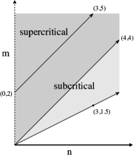
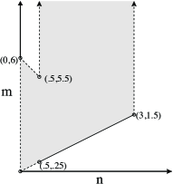
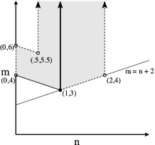
Figure 1: Left: the darker region represents the exponents $(n,m)$ for which the methods of [12] yield short-time existence results like Theorems 1 and 2. The larger, lighter region represents the additional exponents for which we’ve proved our theorems. Middle: For $(n,m)$ in the shaded region, we prove that the strong solutions of Theorem 2 can have finite speed of propagation (Theorem 3). Right: For $(n,m)$ in the shaded region, we construct solutions on the line that blow up in finite time (Theorem 4). The heavy solid line denotes the $(n,m)$ for which this had already been done by [13].

In Theorem 3 we prove that if the initial data $h_{0}$ has compact support then the strong solution of Theorem 2 will have finite speed of propagation. Specifically, if the support of the initial data satisfies $\mbox{supp}(h_{0})\subseteq[-r_{0},r_{0}]\subset(-a,a)$ then there is a nondecreasing function $\Gamma(t)$ and a time $T_{speed}$ such that $\mbox{supp}(h(\cdot,t))\subseteq[-r_{0}-\Gamma(t),r_{0}+\Gamma(t)]\subset(-a,a)$ for every time $t\in[0,T_{speed}]$. For $0<n<2$, we further prove that there is a constant $C$ such that $\Gamma(t)\leqslant Ct^{1/(n+4)}$. This power law behaviour is the same as has been found for $h_{t}=-(|h|^{n}h_{xxx})_{x}$ for $0<n<2$ [5] and $2\leqslant n<3$ [29]; it corresponds to the rate of expansion of the self–similar source–type solution.

The middle plot in Figure 1 presents the $(n,m)$ parameter range for which we were able to prove finite speed of propagation. While we were successful in proving finite speed of propagation for the entire expected range of $m\geqslant n/2$ if $1/2<n<3$, if $0<n\leqslant 1/2$ we could prove it for only a subset of $m\geqslant n/2$. This technical obstruction is discussed further in Section 7. The $n$ values are restricted to $n<3$ because for $n\geq 3$ if initial data has compact support in $(-a,a)$ then it will have infinite entropy and will not be admissible initial data for Theorems 1 and 2.

To prove Theorem 3 we start by proving a local entropy estimate similar to that of [5] for $0<n<2$ and a local energy estimate similar to that of [6, 29] for $1/2<n<3$. Using these and well-chosen ‘‘localization’’ (or ‘‘test’’) functions, we find systems of functional inequalities. In [24], Giacomelli and Shishkov proved an extension of Stampacchia’s lemma to systems of inequalities, we use this to then finish the proof.

A Stampacchia-like lemma for a single inequality was used by [29] to prove finite speed of propagation for $h_{t}=-(|h|^{n}h_{xxx})_{x}$ and [18] proved an extension of Stampacchia’s lemma (also for a single inequality) to study waiting time phenomena. Similar approaches were subsequently used to study finite speed of propagation and waiting time phenomena for related equations, see [1, 19, 25, 27, 42, 23, 39, 40, 41]. Further, there are finite speed of propagation and waiting time results [42, 35] that use the extension of Stampacchia’s lemma to systems of [24] as well as other types of extensions to systems [41].

Having proven finite speed of propagation in Theorem 3, we use this to prove a short-time existence result for the Cauchy problem. Specifically, for the range of exponents $(n,m)$ of Theorem 3 given nonnegative initial data with bounded support in $\mathbb{R}^{1}$ we construct a nonnegative, compactly supported strong solution on $\mathbb{R}^{1}\times[0,T_{0}]$ that satisfies the bounds and regularity of Theorems 1 and 2 (with those bounds taken over $\mathbb{R}^{1}$ rather than $\Omega$). The larger the $H^{1}$ norm of the initial data, the shorter the time $T_{0}$. In Lemma 8.1 we prove that for a subset of these exponents (see Figure 1), the entropy of the solution satisfies a second-moment inequality at time $T_{0}$

$$e^{-\widetilde{B}(T_{0})}\int\limits_{-\infty}^{\infty}{x^{2}\widetilde{G}_{0}(h(x,T_{0}))\,dx}\leqslant\int\limits_{-\infty}^{\infty}{x^{2}\widetilde{G}_{0}(h_{0})\,dx}+\int\limits_{0}^{T_{0}}{e^{-\widetilde{B}(t)}\left(k_{1}\mathcal{E}_{0}(0)+k_{2}\int\limits_{-\infty}^{\infty}{x^{2}h^{2}_{xx}\,dx}\right)\,dt}$$

where $k_{1}=2(4-n)$, $k_{2}=3a_{0}(n-1)/2$, $\mathcal{E}_{0}(0)$ is the energy of the initial data (1.5),

$$\widetilde{G}_{0}(z)=\tfrac{1}{2-n}z^{2-n},\qquad\mbox{and}\qquad\widetilde{B}(t)=\tfrac{a_{1}^{2}|(1-n)(2-n)|}{2a_{0}(m-n+1)^{2}}\int\limits_{0}^{t}{\|h(.,\tau)\|_{L^{\infty}(\Omega)}^{2m-n}\,d\tau}.$$

Note that if $n=1$ then the second-moment inequality for the entropy reduces to the second moment inequality (1.4) used by [13].

‘‘Time-stepping’’ this existence result, we construct a nonnegative, compactly supported, strong solution on $\mathbb{R}^{1}\times[0,T^{*})$ such that our second-moment inequality for the entropy holds for a sequence of times $T_{i}\to T^{*}$. The left-hand side of the inequality is nonnegative. If the initial data has negative energy, then the second term on the right-hand side has an integrand which has the possibility of becoming negative. In Theorem 4 we prove that for a range of $(n,m)$ values (see Figure 1) that if $T^{*}=\infty$ then the constructed solution would yield a right-hand side that becomes negative in finite time, an impossibility. Hence $T^{*}$ must be finite and therefore the $\limsup_{t\to T^{*}}\|h(\cdot,t)\|_{H^{1}}$ must be infinite.

Ideally, we would have proven finite speed of propagation for all $(n,m)$ with $0<n<3$ and all $n/2\leqslant m$ and would have proven the finite time blow up result for all $(n,m)$ with $0<n<3$ and all $m\geqslant n+2$. We believe the obstructions are technical ones.

We close by noting that our blow–up result does not give qualitative information such as proving that there’s a focussing singularity, as suggested by numerical simulations [12]. However, there has been some detailed study of the critical regime $m=n+2$. There, a critical mass $M_{c}$ has been identified [43], there are self-similar, compactly-supported, source-type solutions with masses in $[0,M_{c})$ [3], and there are self-similar, compactly supported, solutions with masses in $(M_{c},M_{1})$ that blow up in finite time [37]. Further, these self-similar blow-up solutions have been shown to be linearly stable [38].

2 Generalized weak solution

We study the existence of a nonnegative weak solution, $h(x,t)$, of the initial–boundary value problem

$$(\textup{P}) h_{t}+\left(f(h)\left(a_{0}h_{xxx}+a_{1}D^{\prime\prime}(h)h_{x}\right)\right)_{x}=0\text{ in }Q_{T},\hfill$$ (2.1)

$$(\textup{P}) \tfrac{\partial^{i}h}{\partial x^{i}}(-a,t)=\tfrac{\partial^{i}h}{\partial x^{i}}(a,t)\text{ for }t>0,\,i=\overline{0,3},\hfill$$ (2.2)

$$(\textup{P}) \qquad\qquad h(0,x)=h_{0}(x)\geqslant 0,\hfill$$ (2.3)

where $a_{0}>0$, $a_{1}\geqslant 0$, $f(h)=|h|^{n}$, $D^{\prime\prime}(h)=|h|^{m-n}$, $n>0$, $m>0$, $\Omega=(-a,a)$, and $Q_{T}=\Omega\times(0,T)$. We consider a weak solution like that considered in [4, 5]:

Definition 2.1 (generalized weak solution).

Let $n>0$, $m>0$, $a_{0}>0$, and $a_{1}\geqslant 0$. A function $h$ is a generalized weak solution of the problem $(\textup{P})$ if

$$h\in C^{1/2,1/8}_{x,t}(\overline{Q}_{T})\cap L^{\infty}(0,T;H^{1}(\Omega)),$$ (2.4)

$$h_{t}\in L^{2}(0,T;(H^{1}(\Omega))^{\prime}),$$ (2.5)

$$h\in C^{4,1}_{x,t}(\mathcal{P}),\,\,\,\sqrt{f(h)}\,\left(a_{0}h_{xxx}+a_{1}D^{\prime\prime}(h)h_{x}\right)\in L^{2}(\mathcal{P}),\,\,$$ (2.6)

where $\mathcal{P}=\overline{Q}_{T}\setminus(\{h=0\}\cup\{t=0\})$ and $h$ satisfies (2.1) in the following sense:

$$\int\limits_{0}^{T}\langle h_{t}(\cdot,t),\phi\rangle\;dt-\iint\limits_{\mathcal{P}}{f(h)(a_{0}h_{xxx}+a_{1}D^{\prime\prime}(h)h_{x})\phi_{x}\,dxdt}\ =0$$ (2.7)

for all $\phi\in C^{1}(Q_{T})$ with $\phi(-a,\cdot)=\phi(a,\cdot)$;

$$h(\cdot,t)\to h(\cdot,0)=h_{0}\mbox{ pointwise \& strongly in $L^{2}(\Omega)$ as $t\to 0$},$$ (2.8)

$$h(-a,t)=h(a,t)\;\forall t\in[0,T]\;\mbox{and}\;\tfrac{\partial^{i}h}{\partial x^{i}}(-a,t)=\tfrac{\partial^{i}h}{\partial x^{i}}(a,t)$$ (2.9)

$$\mbox{for}\;i=\overline{1,3}\;\mbox{at all points of the lateral boundary where $\{h\neq 0\}$.}$$

Because the second term of (2.7) has an integral over $\mathcal{P}$ rather than over $Q_{T}$, the generalized weak solution is ‘‘weaker’’ than a standard weak solution. Also note that the first term of (2.7) uses $h_{t}\in L^{2}(0,T;(H^{1}(\Omega))^{\prime})$; this is different from the definition of weak solution first introduced by Bernis and Friedman [7]; there, the first term was the integral of $h\phi_{t}$ integrated over $Q_{T}$. We do not require a test function $\phi$ to be zero at both ends $t=0$ and $t=T$ that is crucial for our construction of a continuation of the weak solution.

3 Main results

Our main results are: the short-time existence of a nonnegative generalized weak solution (Theorem 1), the short-time existence of a nonnegative strong solution (Theorem 2), finite-speed of propagation and finite-time blow-up for some of these strong solutions (Theorems 3 and 4 respectively).

The short-time existence of generalized weak solutions relies on an integral quantity: $\int G_{0}(h(x,t))\;dx$. This ‘‘entropy’’ was introduced by Bernis and Friedman [7], where

$$G_{0}(z):=\begin{cases}\tfrac{z^{2-n}}{(2-n)(1-n)}&\text{if }n\in(0,1)\cup(2,\infty)\\ \tfrac{z^{2-n}}{(2-n)(1-n)}+z+b&\text{if }n\in(1,2)\\ z\ln z-z+1&\text{ if }n=1\\ -\ln z+z/e&\text{ if }n=2.\end{cases}\Longrightarrow\quad G_{0}^{\prime\prime}(z)=\tfrac{1}{z^{n}}$$ (3.1)

with $b$ chosen to ensure that $G_{0}(z)\geqslant 0$ for all $z\geqslant 0$.

Theorem 1 (Existence).

Let $n>0,\ m\geqslant\tfrac{n}{2}$, $a_{0}>0$, and $a_{1}\geqslant 0$ in equation (1.2). Assume that the nonnegative initial data $h_{0}\in H^{1}(\Omega)$ has finite entropy

$$\int\limits_{\Omega}{G_{0}(h_{0}(x))\,dx}<\infty,$$ (3.2)

where $G_{0}$ is given by (3.1) and either 1) $h_{0}(-a)=h_{0}(a)=0$ or 2) $h_{0}(-a)=h_{0}(a)\neq 0$ and $\tfrac{\partial^{i}h_{0}}{\partial x^{i}}(-a)=\tfrac{\partial^{i}h_{0}}{\partial x^{i}}(a)\text{ holds for }i=1,2,3$. Then for some time $T_{loc}>0$ there exists a nonnegative generalized weak solution $h$ on $Q_{T_{loc}}$ in the sense of the definition 2.1. Furthermore,

$$h\in L^{2}(0,T_{loc};H^{2}(\Omega)).$$ (3.3)

If

$$D_{0}(z)=\begin{cases}\tfrac{z^{m-n+2}}{(m-n+1)(m-n+2)}&\mbox{if}\;m-n\notin\{-2,-1\}\\ -\log(z)&\mbox{if}\;m-n=-2\\ z\log(z)&\mbox{if}\;m-n=-1\end{cases},\quad\Longrightarrow\quad D_{0}^{\prime\prime}(z)=z^{m-n},$$ (3.4)

$$\mathcal{E}_{0}(T):=\int\limits_{\Omega}{\{\tfrac{a_{0}}{2}h_{x}^{2}(x,T)-a_{1}D_{0}(h(x,T))\}\,dx},\qquad B_{1}(T):=\tfrac{a_{1}^{2}}{a_{0}}\int\limits_{0}^{T}{\|h(.,t)\|^{2m-n}_{L^{\infty}(\Omega)}\,dt},$$ (3.5)

and

$$B_{2}(T):=\tfrac{a_{1}^{4}}{2a_{0}^{3}(2m-n+1)^{2}}\int\limits_{0}^{T}\|h(\cdot,t)\|_{\infty}^{4m-n}\;dt+\tfrac{a_{1}^{2}}{2a_{0}(m-n+1)^{2}}\int\limits_{0}^{T}\|h(\cdot,t)\|_{\infty}^{2m-n}\;dt,$$

then the weak solution satisfies

$$\mathcal{E}_{0}(T_{loc})+\iint\limits_{\{h>0\}}{h^{n}(a_{0}h_{xxx}+a_{1}h^{m-n}h_{x})^{2}\,dxdt}\leqslant\mathcal{E}_{0}(0),$$ (3.6)

$$\int\limits_{\Omega}{h_{x}^{2}(x,T_{loc})\,dx}\leqslant e^{B_{1}(T_{loc})}\int\limits_{\Omega}{h_{0x}^{2}(x)\,dx},$$ (3.7)

and

$$\int\limits_{\Omega}{\{h_{x}^{2}(x,T_{loc})+G_{0}(h(x,T_{loc})\}\,dx}\leqslant e^{B_{2}(T_{loc})}\int\limits_{\Omega}{\{h_{0x}^{2}(x)+G_{0}(h_{0}(x))\,dx}.$$ (3.8)

The time of existence, $T_{loc}$, is determined by $a_{0}$, $a_{1}$, $|\Omega|$, $\int h_{0}$, $\|h_{0x}\|_{2}$, and $\int G_{0}(h_{0})$.

There is nothing special about the time $T_{loc}$ in the bounds (3.6), (3.7), and (3.8); given a countable collection of times in $[0,T_{loc}]$, one can construct a weak solution for which these bounds will hold at those times. Also, we note that the analogue of Theorem 4.2 in [7] also holds: there exists a nonnegative weak solution with the integral formulation

$$\int\limits_{0}^{T}\langle h_{t}(\cdot,t),\phi\rangle\;dt+a_{0}\iint\limits_{Q_{T}}(nh^{n-1}h_{x}h_{xx}\phi_{x}+h^{n}h_{xx}\phi_{xx})\;dxdt-a_{1}\iint\limits_{Q_{T}}{h^{m}h_{x}\phi_{x}\;dxdt}=0.$$ (3.9)

We note that the existence theory for the long-wave stable case, $a_{1}<0$, has already been considered by [10, 20].

Theorem 2 states that if the initial data also has finite ‘‘$\alpha$-entropy’’ then a solution can be constructed which satisfies Theorem 1 and has additional regularity. This solution is called a ‘‘strong’’ solution; see [11, 4, 10]. The $\alpha$-entropy, defined below, was discovered by Leo Kadanoff [14]. Let

$$G_{0}^{(\alpha)}(z)=\begin{cases}\tfrac{z^{2-n+\alpha}}{(2-n+\alpha)(1-n+\alpha)}&\mbox{if }\alpha\in(-\infty,n-2)\cup(n-1,\infty)\\ \tfrac{z^{2-n+\alpha}}{(2-n+\alpha)(1-n+\alpha)}+z+c&\mbox{if }\alpha\in(n-2,n-1)\\ z\ln z-z+1&\mbox{if }\alpha=n-1\\ -\ln z+z/e&\mbox{if }\alpha=n-2,\end{cases}G_{0}^{(\alpha)^{\prime\prime}}(z)=\tfrac{z^{\alpha}}{z^{n}}$$ (3.10)

where $c$ is chosen to ensure that $G_{0}^{(\alpha)}(z)\geqslant 0$ for all $z\geqslant 0$.

Theorem 2 (Regularity).

Assume the initial data $h_{0}$ satisfies the hypotheses of Theorem 1 and also has finite $\alpha$-entropy for some $\alpha\in(-1/2,1)$, $\alpha\neq 0$,

$$\int\limits_{\Omega}{G_{0}^{(\alpha)}(h_{0}(x))\,dx}<\infty.$$ (3.11)

Then for some time time $T_{loc}^{(\alpha)}\in(0,T_{loc}]$ there exists a nonnegative generalized weak solution on $Q_{T_{loc}^{(\alpha)}}$ that satisfies Theorem 1 and has the additional regularity

$$h^{\tfrac{\alpha+2}{2}}\in L^{2}(0,T_{loc}^{(\alpha)};H^{2}(\Omega))\text{ and }h^{\tfrac{\alpha+2}{4}}\in L^{2}(0,T_{loc}^{(\alpha)};W^{1}_{4}(\Omega)).$$ (3.12)

Theorem 3 (Finite Speed of Propagation).

Consider the range of exponents $0<n\leqslant\tfrac{1}{2}$ and $n/2<m<6-n$ or $\tfrac{1}{2}<n<3$ and $m\geqslant n/2$ (see Figure 1). Assume the initial data satisfies the hypotheses of Theorem 2 and also has compact support in $(-a,a)$: $\mbox{supp}(h_{0})\subseteq[-r_{0},r_{0}]\subset(-a,a)$. Then there exists a time $0<T_{speed}\leqslant T_{loc}^{(\alpha)}$ and a nondecreasing function $\Gamma(t)\in C([0,T_{speed}])$ such that the strong solution from Theorem 2, has finite speed propagation, i.e.

$$\mbox{supp}(h(\cdot,t))\subseteq[-r_{0}-\Gamma(t),r_{0}+\Gamma(t)]\subset(-a,a)$$

for all $t\in[0,T_{speed}]$. Furthermore, if $0<n<2$ there exists a constant $C$ which depends on $n$, $m$, $\alpha$, and $\int h_{0}$ such that $\Gamma(t)\leqslant Ct^{1/(n+4)}$.

Theorem 4 (Finite Time Blow Up).

Consider the range of exponents $0<n\leqslant\tfrac{1}{2}$ and $4-n\leqslant m<6-n$ or $\tfrac{1}{2}<n\leqslant 1$ and $m\geqslant 4-n$ or $1<n<2$ and $m\geqslant n+2$ (see Figure 1). Assume the nonnegative initial data $h_{0}$ has compact support, negative energy (3.5)

$$\mathcal{E}_{0}(0)=\int\limits_{-\infty}^{\infty}{\{\tfrac{a_{0}}{2}h_{0x}^{2}-a_{1}D_{0}(h_{0})\}\,dx}<0,$$

and satisfies the hypotheses of Theorem 2 with $\Omega=\mathbb{R}^{1}$. Then there exists a finite time $T^{*}<\infty$ and a nonnegative, compactly supported, strong solution $h$ on $\mathbb{R}^{1}\times[0,T^{*})$ such that

$$\mathop{\limsup}\limits_{t\to T^{*}}\|h(.,t)\|_{H^{1}(\mathbb{R}^{1})}=\mathop{\limsup}\limits_{t\to T^{*}}\|h(.,t)\|_{L^{\infty}(\mathbb{R}^{1})}=+\infty.$$ (3.13)

The solution satisfies the bounds of Theorems 1 and 2 with $\Omega=\mathbb{R}^{1}$.

4 Proof of Existence of Generalized Solutions

Our proof of existence of generalized weak solutions defined in the section 2 follows the main concept of the proof from [7].

4.1 Regularized Problem

Given $\delta,\varepsilon>0$, a regularized parabolic problem, similar to that of Bernis and Friedman [7], is considered:

$$(\textup{P}_{\delta,\varepsilon}) h_{t}+\left({f_{\delta\varepsilon}(h)(a_{0}h_{xxx}+a_{1}D^{\prime\prime}_{\varepsilon}(h)h_{x})}\right)_{x}=0,\qquad\hfill$$ (4.1)

$$(\textup{P}_{\delta,\varepsilon}) \tfrac{\partial^{i}h}{\partial x^{i}}(-a,t)=\tfrac{\partial^{i}h}{\partial x^{i}}(a,t)\text{ for }t>0,\,i=\overline{0,3},\hfill$$ (4.2)

$$(\textup{P}_{\delta,\varepsilon}) \qquad\qquad h(x,0)=h_{0,\varepsilon}(x)\hfill$$ (4.3)

where

$$f_{\delta\varepsilon}(z):=f_{\varepsilon}(z)+\delta=\tfrac{|z|^{4+n}}{|z|^{4}+\varepsilon|z|^{n}}+\delta,\ D^{\prime\prime}_{\varepsilon}(z):=\tfrac{|z|^{m-n}}{1+\varepsilon|z|^{m-n}},\varepsilon>0,\delta>0.$$ (4.4)

We note that $f_{\delta\varepsilon}\in C^{1+\gamma}(\mathbb{R}^{1})$ and $f_{\delta\varepsilon}D^{\prime\prime}_{\varepsilon}\in C^{1+\gamma}(\mathbb{R}^{1})$ for some $\gamma\in(0,1)$. The $\delta>0$ in (4.4) makes the problem (4.1) regular (i.e. uniformly parabolic). The parameter $\varepsilon$ is an approximating parameter which has the effect of increasing the degeneracy from $f(h)\sim|h|^{n}$ to $f_{\varepsilon}(h)\sim h^{4}$. For $\varepsilon>0$, the nonnegative initial data, $h_{0}$, is approximated via

$$\begin{gathered}h_{0}+\varepsilon^{\theta}\leq h_{0,\varepsilon}\in C^{4+\gamma}(\overline{\Omega})\text{ for some }0<\theta<\tfrac{2}{5},\\ \tfrac{\partial^{i}h_{0,\varepsilon}}{\partial x^{i}}(-a)=\tfrac{\partial^{i}h_{0,\varepsilon}}{\partial x^{i}}(a)\text{ for }i=\overline{0,3},\\ h_{0,\varepsilon}\to h_{0}\text{ strongly in }H^{1}(\Omega)\text{ as }\varepsilon\to 0.\end{gathered}$$ (4.5)

The effect of $\varepsilon>0$ in (4.5) is to both ‘‘lift’’ the initial data, making it positive, and to smooth the initial data from $H^{1}(\Omega)$ to $C^{4+\gamma}(\Omega)$.

By Eĭdelman [22, Theorem 6.3, p.302], the regularized problem has a unique classical solution $h_{\delta\varepsilon}\in C_{x,t}^{4+\gamma,1+\gamma/4}(\Omega\times[0,\tau_{\delta\varepsilon}])$ for some time $\tau_{\delta\varepsilon}>0$. For any fixed value of $\delta$ and $\varepsilon$, by Eĭdelman [22, Theorem 9.3, p.316] if one can prove a uniform in time an a priori bound $|h_{\delta\varepsilon}(x,t)|\leqslant A_{\delta\varepsilon}<\infty$ for some longer time interval $[0,T_{loc,\delta\varepsilon}]\quad(T_{loc,\delta\varepsilon}>\tau_{\delta\varepsilon}$) and for all $x\in\Omega$ then Schauder-type interior estimates [22, Corollary 2, p.213] imply that the solution $h_{\delta\varepsilon}$ can be continued in time to be in $C_{x,t}^{4+\gamma,1+\gamma/4}(\Omega\times[0,T_{loc,\delta\varepsilon}])$.

Although the solution $h_{\delta\varepsilon}$ is initially positive, there is no guarantee that it will remain nonnegative. The goal is to take $\delta\to 0$, $\varepsilon\to 0$ in such a way that a) $T_{loc,\delta\varepsilon}\to T_{loc}>0$, b) the solutions $h_{\delta\varepsilon}$ converge to a (nonnegative) limit, $h$, which is a generalized weak solution, and c) $h$ inherits certain a priori bounds. This is done by proving various a priori estimates for $h_{\delta\varepsilon}$ that are uniform in $\delta$ and $\varepsilon$ and hold on a time interval $[0,T_{loc}]$ that is independent of $\delta$ and $\varepsilon$. As a result, $\{h_{\delta\varepsilon}\}$ will be a uniformly bounded and equicontinuous (in the $C_{x,t}^{1/2,1/8}$ norm) family of functions in $\bar{\Omega}\times[0,T_{loc}]$. Taking $\delta\to 0$ will result in a family of functions $\{h_{\varepsilon}\}$ that are classical, positive, unique solutions to the regularized problem with $\delta=0$. Taking a subsequence of $\varepsilon$ going to zero will then result in the desired generalized weak solution $h$. This last step is where the possibility of nonunique weak solutions arise; see [4] for simple examples of how such a construction applied to $h_{t}=-(|h|^{n}h_{xxx})_{x}$ can result in there being two different solutions arising from the same initial data.

4.2 A priori estimates

We start by proving a priori estimates for classical solutions of the regularized problem (4.1)–(4.5). Appendix A contains the proofs of the lemmas in this section.

We introduce function $G_{\delta\varepsilon}$ chosen such that

$$G^{\prime\prime}_{\delta\varepsilon}(z)=\tfrac{1}{f_{\delta\varepsilon}(z)}\quad\mbox{and}\quad G_{\delta\varepsilon}(z)\geqslant 0\quad\forall z\in\mathbb{R}^{1}.$$ (4.6)

This is analogous to the ‘‘entropy’’ function (3.1) introduced by Bernis and Friedman [7].

Lemma 4.1.

Let $n>0$ and $m\geqslant n/2$. There exist $\delta_{0}>0$, $\varepsilon_{0}>0$, and time $T_{loc}>0$ such that if $\delta\in[0,\delta_{0})$, $\varepsilon\in(0,\varepsilon_{0})$ and $h_{\delta\varepsilon}$ is a classical solution of the problem (4.1)–(4.5) with initial data $h_{0,\delta\varepsilon}$ that is built from a nonnegative function $h_{0}$ satisfying the hypotheses of Theorem 1 then for any $T\in[0,T_{loc}]$ the following inequalities hold true:

$$\int\limits_{\Omega}{\{h_{\delta\varepsilon,x}^{2}(x,T)+\tfrac{a_{1}^{2}}{2a_{0}^{2}}(1+\delta)G_{\delta\varepsilon}(h_{\delta\varepsilon}(x,T))\}\,dx}$$ (4.7)

$$\hskip 72.26999pt+a_{0}\iint\limits_{Q_{T}}{f_{\delta\varepsilon}(h_{\delta\varepsilon})h^{2}_{\delta\varepsilon,xxx}\,dxdt}\leqslant K_{1}<\infty,$$

$$\int\limits_{\Omega}G_{\delta\varepsilon}(h_{\delta\varepsilon}(x,T))\;dx+\tfrac{a_{0}}{2}\iint\limits_{Q_{T}}h_{\delta\varepsilon,xx}^{2}\;dxdt\leqslant K_{2}<\infty.$$ (4.8)

The energy $\mathcal{E}_{\delta\varepsilon}(t)$ (see (3.5)) satisfies:

$$\mathcal{E}_{\delta\varepsilon}(T)+\iint\limits_{Q_{T}}{f_{\delta\varepsilon}(h_{\delta\varepsilon})(a_{0}h_{\delta\varepsilon,xxx}+a_{1}D^{\prime\prime}_{\varepsilon}(h_{\delta\varepsilon})h_{\delta\varepsilon,x})^{2}}\;dxdt=\mathcal{E}_{\delta\varepsilon}(0).$$ (4.9)

The time $T_{loc}$ and the constants $K_{1}$, and $K_{2}$ are independent of $\delta$ and $\varepsilon$.

The existence of $\delta_{0}$, $\varepsilon_{0}$, $T_{loc}$, $K_{1}$, $K_{2}$, and $C_{0}$ is constructive; how to find them and what quantities determine them is shown in Section A.

Lemma 4.1 yields uniform-in-$\delta$-and-$\varepsilon$ bounds for $\int h_{\delta\varepsilon,x}^{2}$, $\int G_{\delta\varepsilon}(h_{\delta\varepsilon})$, $\iint f_{\delta\varepsilon}(h_{\delta\varepsilon})h_{\delta\varepsilon,xxx}^{2}$, and $\iint h_{\delta\varepsilon,xx}^{2}$ which will be key in constructing a nonnegative generalized weak solution. However, these bounds are found in a different manner than in earlier work for the equation $h_{t}=-(|h|^{n}h_{xxx})_{x}$, for example. Although the inequality (4.8) is unchanged, the inequality (4.7) has an extra term involving $G_{\delta\varepsilon}$. In the proof, this term was introduced to control additional, lower–order terms. This idea of a ‘‘blended’’ $\|h_{x}\|_{2}$–entropy bound was first introduced by Shishkov and Taranets especially for long-wave stable thin film equations with convection [34].

Lemma 4.2.

Assume $\varepsilon_{0}$ and $T_{loc}$ are from Lemma 4.1, $\delta=0$, and $\varepsilon\in(0,\varepsilon_{0})$. If $h_{\varepsilon}$ is a positive, classical solution of the problem (4.1)–(4.5) with initial data $h_{0,\varepsilon}$ satisfying Lemma 4.1 then

$$\int\limits_{\Omega}{h_{\varepsilon,x}^{2}(x,T)\,dx}\leqslant e^{B_{1,\varepsilon}(T)}\int\limits_{\Omega}{h_{0\varepsilon,x}^{2}\,dx},$$ (4.10)

$$\int\limits_{\Omega}{\{h_{\varepsilon,x}^{2}(x,T)+G_{\varepsilon}(h_{\varepsilon}(x,T))\}\,dx}\leqslant e^{B_{2,\varepsilon}(T)}\int\limits_{\Omega}{\{h_{0\varepsilon,x}^{2}+G_{\varepsilon}(h_{0,\varepsilon})\}\,dx}$$ (4.11)

hold true for all $T\in[0,T_{loc}]$. Here

$$B_{1,\varepsilon}(T):=\tfrac{a_{1}^{2}}{a_{0}}\int\limits_{0}^{T}\|h_{\varepsilon}(\cdot,t)\|_{\infty}^{2m-n}\;dt,$$

$$B_{2,\varepsilon}(T):=\tfrac{a_{1}^{4}}{2a_{0}^{3}(2m-n+1)^{2}}\int\limits_{0}^{T}\|h_{\varepsilon}(\cdot,t)\|_{\infty}^{4m-n}\;dt+\tfrac{a_{1}^{2}}{2a_{0}(m-n+1)^{2}}\int\limits_{0}^{T}\|h_{\varepsilon}(\cdot,t)\|_{\infty}^{2m-n}\;dt.$$

The final a priori bound uses the following functions, parametrized by $\alpha$, chosen such that $G_{\varepsilon}^{(\alpha)}\geqslant 0$ and $G_{\varepsilon}^{(\alpha)\prime\prime}(z)=z^{\alpha}/f_{\varepsilon}(z)$:

$$G_{\varepsilon}^{(\alpha)}(z)=\begin{cases}\tfrac{z^{2-n+\alpha}}{(2-n+\alpha)(1-n+\alpha)}+\varepsilon\tfrac{z^{\alpha-2}}{(\alpha-3)(\alpha-2)}&\mbox{if }\alpha\in(-\infty,n-2)\cup(n-1,\infty)\\ \tfrac{z^{2-n+\alpha}}{(2-n+\alpha)(1-n+\alpha)}+\varepsilon\tfrac{z^{\alpha-2}}{(\alpha-3)(\alpha-2)}+z+c&\mbox{if }\alpha\in(n-2,n-1)\\ z\ln z-z+1+\varepsilon\tfrac{z^{\alpha-2}}{(\alpha-3)(\alpha-2)}&\mbox{if }\alpha=n-1\\ -\ln z+z/e+\varepsilon\tfrac{z^{\alpha-2}}{(\alpha-3)(\alpha-2)}&\mbox{if }\alpha=n-2,\end{cases}$$ (4.12)

Lemma 4.3.

Assume $\varepsilon_{0}$ and $T_{loc}$ are from Lemma 4.1, $\delta=0$, and $\varepsilon\in(0,\varepsilon_{0})$. Assume $h_{\varepsilon}$ is a positive, classical solution of the problem (4.1)–(4.5) with initial data $h_{0,\varepsilon}$ that is built from a nonnegative function $h_{0}$ satisfying the hypotheses of Theorem 2 then there exists $K_{3}$, $\varepsilon_{0}^{(\alpha)}$ and $T_{loc}^{(\alpha)}$ with $0<\varepsilon_{0}^{(\alpha)}\leqslant\varepsilon_{0}$ and $0<T_{loc}^{(\alpha)}\leqslant T_{loc}$ such that

$$\int\limits_{\Omega}{\{h_{\varepsilon,x}^{2}(x,T)+G_{\varepsilon}^{(\alpha)}(h_{\varepsilon}(x,T))\}\,dx}+\iint\limits_{Q_{T}}\left[\beta h_{\varepsilon}^{\alpha}h_{\varepsilon,xx}^{2}+\gamma h_{\varepsilon}^{\alpha-2}h_{\varepsilon,x}^{4}\right]\;dx\,dt\leqslant K_{3}<\infty$$ (4.13)

holds for all $T\in[0,T_{loc}^{(\alpha)}]$. $K_{3}$ is determined by $\alpha$, $\varepsilon_{0}$, $a_{0}$, $a_{1}$, $\Omega$ and $h_{0}$. Here,

$$\beta=\begin{cases}a_{0}&\mbox{if }0<\alpha<1,\\ a_{0}\tfrac{1+2\alpha}{4(1-\alpha)}&\mbox{if }-1/2<\alpha<0\end{cases}$$

and

$$\gamma=\begin{cases}a_{0}\tfrac{\alpha(1-\alpha)}{6}&\mbox{if }0<\alpha<1,\\ a_{0}\tfrac{(1+2\alpha)(1-\alpha)}{36}&\mbox{if }-1/2<\alpha<0.\end{cases}$$

Furthermore,

$$h_{\varepsilon}^{\tfrac{\alpha+2}{2}}\in B_{R_{1}}(0)\subset L^{2}(0,T_{loc};H^{2}(\Omega))\quad\mbox{and}\quad h_{\varepsilon}^{\tfrac{\alpha+2}{4}}\in B_{R_{2}}(0)\subset\in L^{2}(0,T_{loc};W^{1}_{4}(\Omega))$$ (4.14)

where the radii $R_{1}$ and $R_{2}$ are independent of $\varepsilon$.

The $\alpha$–entropy, $\int G_{0}^{(\alpha)}(h)\;dx$, was first introduced for $\alpha=-1/2$ in [14] and an a priori bound like that of Lemma 4.3 and regularity results like those of Theorem 2 were found simultaneously and independently in [4] and [11].

4.3 Proof of existence and regularity of solutions

Bound (4.7) yields uniform $L^{\infty}$ control for classical solutions $h_{\delta\varepsilon}$, allowing the time of existence $T_{loc,\delta\varepsilon}$ to be taken as $T_{loc}$ for all $\delta\in(0,\delta_{0})$ and $\varepsilon\in(0,\varepsilon_{0})$. The existence theory starts by constructing a classical solution $h_{\delta\varepsilon}$ on $[0,T_{loc}]$ that satisfy the hypotheses of Lemma 4.1 if $\delta\in(0,\delta_{0})$ and $\varepsilon\in(0,\varepsilon_{0})$. The a priori bounds of Lemma 4.1 then allow one to take the regularizing parameter, $\delta$, to zero and prove that there is a limit $h_{\varepsilon}$ and that $h_{\varepsilon}$ is a generalized weak solution. One then proves additional regularity for $h_{\varepsilon}$; specifically that it is strictly positive, classical, and unique. It then follows that the a priori bounds given by Lemmas 4.1, 4.2, and 4.3 apply to $h_{\varepsilon}$. This allows one to take the approximating parameter, $\varepsilon$, to zero and construct the desired generalized weak solution of Theorems 1 and 2:

Lemma 4.4.

Assume that the initial data $h_{0,\varepsilon}$ satisfies (4.5) and is built from a nonnegative function $h_{0}$ that satisfies the hypotheses of Theorem 1. Fix $\delta=0$ and $\varepsilon\in(0,\varepsilon_{0})$ where $\varepsilon_{0}$ is from Lemma 4.1. Then there exists a unique, positive, classical solution $h_{\varepsilon}$ on $[0,T_{loc}]$ of problem ($\mbox{P}_{0,\varepsilon}$), see (4.1)–(4.5), with initial data $h_{0,\varepsilon}$ where $T_{loc}$ is the time from Lemma 4.1.

The proof uses a number of arguments like those presented by Bernis & Friedman [7] and we refer to that article as much as possible.

Proof.

Fix $\varepsilon\in(0,\varepsilon_{0})$ and assume $\delta\in(0,\delta_{0})$. Because $G_{\delta\varepsilon}(z)\geqslant 0$, the bound (4.7) yields a uniform-in-$\delta$-and-$\varepsilon$ upper bound on $|h_{\delta\varepsilon}(x,T)|$ for $(x,T)\in\overline{\Omega}\times[0,T_{loc}]$. As discussed in Subsection 4.1, this allows the classical solution $h_{\delta\varepsilon}$ to be extended from $[0,\tau_{\delta\varepsilon}]$ to $[0,T_{loc}]$.

By Section 2 of [7], the a priori bound (4.7) on $\|h_{x}(\cdot,T_{loc})\|_{2}$ implies that $h_{\delta\varepsilon}\in C^{1/2,1/8}_{x,t}(\overline{Q_{T_{loc}}})$ and that $\{h_{\delta\varepsilon}\}$ is a uniformly bounded, equicontinuous family in $\overline{Q_{T_{loc}}}$. By the Arzela-Ascoli theorem, there is a subsequence $\{\delta_{k}\}$, so that $h_{\delta_{k}\varepsilon}$ converges uniformly to a limit $h_{\varepsilon}\in C^{1/2,1/8}_{x,t}(\overline{Q_{T_{loc}}})$.

We now argue that $h_{\varepsilon}$ is a generalized weak solution, using methods similar to those of [7, Theorem 3.1].

By construction, $h_{\varepsilon}$ is in $C^{1/2,1/8}_{x,t}(\overline{Q_{T_{loc}}})$, satisfying the first part of (2.4). The strong convergence $h_{\varepsilon}(\cdot,t)\to h_{\varepsilon}(\cdot,0)$ in $L^{2}(\Omega)$ follows immediately. The uniform convergence of $h_{\delta_{k}\varepsilon}$ to $h_{\varepsilon}$ implies the pointwise convergence $h(\cdot,t)\to h(\cdot,0)=h_{0}$, and so $h_{\varepsilon}$ satisfies (2.8).

Because $h_{\delta\varepsilon}$ is a classical solution,

$$\iint\limits_{Q_{T}}{h_{\delta\varepsilon,t}\phi\;dxdt}-\iint\limits_{Q_{T_{loc}}}{f_{\delta\varepsilon}(h_{\delta\varepsilon})(a_{0}h_{\delta\varepsilon,xxx}+a_{1}D^{\prime\prime}_{\varepsilon}(h_{\delta\varepsilon})h_{\delta\varepsilon,x})\phi_{x}\;dxdt}=0.$$ (4.15)

The bound (4.7) yields a uniform bound on

$$\delta\iint\limits_{Q_{T_{loc}}}h_{\delta\varepsilon,xxx}^{2}\;dxdt$$

for $\delta\in(0,\delta_{0})$. It follows that

$$\delta_{k}\iint\limits_{Q_{T_{loc}}}(a_{0}h_{\delta\varepsilon,xxx}+a_{1}D^{\prime\prime}_{\varepsilon}(h_{\delta\varepsilon})h_{\delta\varepsilon,x})\phi_{x}\,dxdt\to 0\qquad\mbox{as $\delta_{k}\to 0$.}$$

Introducing the notation

$$H_{\delta\varepsilon}:=f_{\delta\varepsilon}(h_{\delta\varepsilon})(a_{0}h_{\delta\varepsilon,xxx}+a_{1}D^{\prime\prime}_{\varepsilon}(h_{\delta\varepsilon})h_{\delta\varepsilon,x})$$ (4.16)

the integral formulation (4.15) can be written as

$$\iint\limits_{Q_{T}}{h_{\delta\varepsilon,t}\phi dxdt}=\iint\limits_{Q_{T_{loc}}}H_{\delta\varepsilon}(x,t)\phi_{x}(x,t)\;dxdt.$$ (4.17)

By the $L^{\infty}$ control of $h_{\delta\varepsilon}$ and the energy bound (4.9), $H_{\delta\varepsilon}$ is uniformly bounded in $L^{2}(Q_{T_{loc}})$. Taking a further subsequence of $\{\delta_{k}\}$ yields $H_{\delta_{k}\varepsilon}$ converging weakly to a function $H_{\varepsilon}$ in $L^{2}(Q_{T_{loc}})$. The regularity theory for uniformly parabolic equations implies that $h_{\delta\varepsilon,t}$, $h_{\delta\varepsilon,x}$, $h_{\delta\varepsilon,xx}$, $h_{\delta\varepsilon,xxx}$, and $h_{\delta\varepsilon,xxxx}$ converge uniformly to $h_{\varepsilon,t}$, …, $h_{\varepsilon,xxxx}$ on any compact subset of $\{h_{\varepsilon}>0\}$, implying (2.9) and the first part of (2.6). Note that because the initial data $h_{0,\delta\varepsilon}$ is in $C^{4}$ the regularity extends all the way to $t=0$ which is excluded in the definition of $\mathcal{P}$ in (2.6).

The energy $\mathcal{E}_{\delta\varepsilon}(T_{loc})$ is not necessarily positive. However, the a priori bound (4.7), combined with the $L^{\infty}$ control on $h_{\delta\varepsilon}$, ensures that $\mathcal{E}_{\delta\varepsilon}(T_{loc})$ has a uniform lower bound. As a result, the bound (4.9) yields a uniform bound on

$$\iint\limits_{Q_{T_{loc}}}f_{\delta\varepsilon}\left(h_{\delta\varepsilon})(a_{0}h_{\delta\varepsilon,xxx}+a_{1}D^{\prime\prime}_{\varepsilon}(h_{\delta\varepsilon})h_{\delta\varepsilon,x}\right)^{2}\;dxdt.$$

Using this, one can argue that for any $\sigma>0$

$$\iint\limits_{\{h_{\varepsilon}<\sigma\}}\left|H_{\delta_{k}\varepsilon}\phi_{x}\right|\;dxdt\leqslant C\sigma^{n/2}$$

for some $C$ independent of $\delta$, $\varepsilon$, and $\sigma$. Taking $\delta_{k}\to 0$ and using that $\sigma$ is arbitrary, we conclude

$$H_{\delta_{k}\varepsilon}\to H_{\varepsilon}=f_{\varepsilon}\left(h_{\varepsilon})(a_{0}h_{\varepsilon,xxx}+a_{1}D^{\prime\prime}_{\varepsilon}(h_{\delta\varepsilon})h_{\varepsilon,x}\right)\,\chi_{\{h_{\varepsilon}>0\}}.$$

As a result, taking $\delta_{k}\to 0$ in (4.17) implies $h_{\varepsilon}$ satisfies (2.7) and the second part of (2.6).

The bound (4.7) yields a uniform bound on $\int h_{\delta\varepsilon,x}^{2}(x,T)\;dx$ for every $T\in[0,T_{loc}]$. As a result, $\{h_{\delta_{k}\varepsilon}\}$ is uniformly bounded in

$$L^{\infty}(0,T_{loc};H^{1}(\Omega)).$$

Therefore, another refinement of the sequence $\{\delta_{k}\}$ yields $\{h_{\delta_{k}\varepsilon}\}$ weakly convergent in this space. As a result, $h_{\varepsilon}\in L^{\infty}(0,T_{loc};H^{1}(\Omega))$ and the second part of (2.4) holds.

Having proven then $h_{\varepsilon}$ is a generalized weak solution, we now prove that $h_{\varepsilon}$ is a strictly positive, classical, unique solution. This uses the entropy $\int G_{\delta\varepsilon}(h_{\delta\varepsilon})$ and the a priori bound (4.8). This bound is, up to the coefficient $a_{0}$, identical to the a priori bound (4.17) in [7]. By construction, the initial data $h_{0,\varepsilon}$ is positive (see (4.5)), hence $\int G_{\varepsilon}(h_{0,\varepsilon})\;dx<\infty$. Also, by construction $f_{\varepsilon}(z)\sim z^{4}$ for $z\ll 1$. This implies that the generalized weak solution $h_{\varepsilon}$ is strictly positive [7, Theorem 4.1]. Because the initial data $h_{0,\varepsilon}$ is in $C^{4}(\bar{\Omega})$, it follows that $h_{\varepsilon}$ is a classical solution in $C^{4,1}_{x,t}(\overline{Q_{T_{loc}}})$. This implies that $h_{\varepsilon}(\cdot,t)\to h_{\varepsilon}(\cdot,0)$ strongly in $C^{1}(\bar{\Omega})$. The proof of Theorem 4.1 in [7] then implies that $h_{\varepsilon}$ is unique. ∎

Proof of Theorem 1.

As in the proof of Lemma 4.4, following [7], there is a subsequence $\{\varepsilon_{k}\}$ such that $h_{\varepsilon_{k}}$ converges uniformly to a function $h\in C^{1/2,1/8}_{x,t}$ which is a generalized weak solution in the sense of Definition 2.1 with $f(h)=|h|^{n}$.

The initial data is assumed to have finite entropy: $\int G_{0}(h_{0})<\infty$ where $G_{0}$ is given by (3.1). This, combined with $f(h)=|h|^{n}$, implies that the generalized weak solution $h$ is nonnegative and, if $n\in[2,4)$ the set of points $\{h=0\}$ in $Q_{T_{loc}}$ has zero measure and $h$ is positive, smooth, and unique if $n\geqslant 4$ [7, Theorem 4.1].

To prove (3.6), start by taking $T=T_{loc}$ in the a priori bound (4.9). As $\varepsilon_{k}\to 0$, the right-hand side of (4.9) is unchanged. Now, consider the $\varepsilon_{k}\to 0$ limit of

$$\mathcal{E}_{\varepsilon_{k}}(T_{loc})=\int\limits_{\Omega}{(\tfrac{a_{0}}{2}h_{\varepsilon_{k},x}^{2}(x,T_{loc})-a_{1}D_{\varepsilon_{k}}(h_{\varepsilon_{k}}(x,T_{loc})))\,dx},$$

where $D_{\varepsilon}$ is defined in (4.4). By the uniform convergence of $h_{\varepsilon_{k}}$ to $h$, the second term in the energy converges strongly as $\varepsilon_{k}\to 0$. Hence the bound (4.9) yields a uniform bound on $\{\int_{\Omega}h_{\varepsilon_{k},x}^{2}(x,T_{loc})\;dx\}$. Taking a further refinement of $\{\varepsilon_{k}\}$, yields $h_{\varepsilon_{k},x}(\cdot,T_{loc})$ converging weakly in $L^{2}(\Omega)$. In a Hilbert space, the norm of the weak limit is less than or equal to the $\liminf$ of the norms of the functions in the sequence, hence $\mathcal{E}_{0}(T_{loc})\leqslant\liminf_{\varepsilon_{k}\to 0}\mathcal{E}_{\varepsilon_{k}}(T_{loc}).$ A uniform bound on $\iint f_{\varepsilon}(h_{\varepsilon})\left(a_{0}h_{\varepsilon,xxx}+\dots\right)^{2}\;dx$ also follows from (4.9). Hence $\sqrt{f_{\varepsilon_{k}}(h_{\varepsilon_{k}})}\left(a_{0}h_{\varepsilon_{k},xxx}+\dots\right)$ converges weakly in $L^{2}(Q_{T_{loc}})$, after taking a further subsequence. We write the weak limit as two integrals: one over $\{h=0\}$ and one over $\{h>0\}$. We can determine the weak limit on $\{h>0\}$: as in the proof of Lemma 4.4, the regularity theory for uniformly parabolic equations allows one to argue that the weak limit is $h^{n/2}\left(a_{0}h_{xxx}+\dots\right)$ on $\{h>0\}$. Using that 1) the norm of the weak limit is less than or equal to the $\liminf$ of the norms of the functions in the sequence and that 2) the $\liminf$ of a sum is greater than or equal to the sum of the $\liminf$s and dropping the nonnegative term arising from the integral over $\{h=0\}$ results in the desired bound (3.6).

It follows from (4.8) that $h_{\varepsilon_{k},xx}$ converges weakly to some $v$ in $L^{2}(Q_{T_{loc}})$, combining with strong convergence in $L^{2}(0,T;H^{1}(\Omega))$ of $h_{\varepsilon_{k}}$ to $h$ by Lemma D.1 and with the definition of weak derivative, we obtain that $v=h_{xx}$ and $h\in L^{2}(0,T_{loc};H^{2}(\Omega))$ that implies (3.3). Hence $h_{\varepsilon,t}\to h_{t}\text{ weakly in }L^{2}(0,T;(H^{1}(\Omega))^{\prime})$ that implies (2.5). By Lemma D.2 we also have $h\in C([0,T_{loc}],L^{2}(\Omega))$. ∎

Proof of Theorem 2.

Fix $\alpha\in(-1/2,1)$. The initial data $h_{0}$ is assumed to have finite entropy $\int G_{0}^{(\alpha)}(h_{0}(x))\;dx<\infty$, hence Lemma 4.3 holds for the approximate solutions $\{h_{\varepsilon_{k}}\}$ where this sequence of approximate solutions is assumed to be the one at the end of the proof of Theorem 1. By (4.14),

$$\left\{h_{\varepsilon_{k}}^{\tfrac{\alpha+2}{2}}\right\}\quad\mbox{is uniformly bounded in $\varepsilon_{k}$ in $L^{2}(0,T_{loc};H^{2}(\Omega))$}$$

and

$$\left\{h_{\varepsilon_{k}}^{\tfrac{\alpha+2}{4}}\right\}\quad\mbox{is uniformly bounded in $\varepsilon_{k}$ in $L^{2}(0,T_{loc};W^{1}_{4}(\Omega))$}.$$

Taking a further subsequence in $\{\varepsilon_{k}\}$, it follows from the proof of [17, Lemma 2.5, p.330] that these sequences converge weakly in $L^{2}(0,T_{loc};H^{2}(\Omega))$ and $L^{2}(0,T_{loc};W^{1}_{4}(\Omega))$, to $h^{\tfrac{\alpha+2}{2}}$ and $h^{\tfrac{\alpha+2}{4}}$ respectively. ∎

5 The subcritical regime: long–time existence of solutions

Lemma 5.1.

Let $h\in H^{1}(\Omega)$ be a nonnegative function and let $M=\int\limits_{\Omega}{h(x)\,dx}$. Then

$$\|h\|_{L^{p}(\Omega)}^{p}\leqslant k_{1}M^{\tfrac{p+2}{3}}\biggl{(}\int\limits_{\Omega}{h^{2}_{x}\,dx}\biggr{)}^{\tfrac{p-1}{3}}+k_{2}M^{p},\ \ p\geqslant 1,$$ (5.1)

where $k_{1}=2^{\tfrac{4-p}{3}}3^{\tfrac{2(p-1)}{3}}(1-\epsilon)^{-1}$, $k_{2}=|\Omega|^{1-p}(1-(1-\epsilon)^{\tfrac{1}{p-1}})^{1-p}$, and $\epsilon\in(0,1)$.

Note that by taking $h$ to be a constant function, one finds that the constant $k_{2}M^{p}$ in (5.1) is sharp when $\epsilon\to 1$.

Proof.

Let $v=h-M/|\Omega|$. By (A.3),

$$\|v\|_{L^{p}(\Omega)}^{p}\leqslant(\tfrac{3}{2})^{\tfrac{2(p-1)}{3}}\biggl{(}\int\limits_{\Omega}{v^{2}_{x}\,dx}\biggr{)}^{\tfrac{p-1}{3}}\biggl{(}\int\limits_{\Omega}{|v|\,dx}\biggr{)}^{\tfrac{p+2}{3}}.$$

Hence, due to the inequality

$$|a-b|^{p}\geqslant(1-\epsilon)a^{p}-c_{0}(\epsilon,p)b^{p}$$

for any $a\geqslant 0,\ b\geqslant 0,\ p>1,\ \epsilon\in(0,1)$, $c_{0}(\epsilon,p)\geqslant\tfrac{1-\epsilon}{(1-(1-\epsilon)^{\tfrac{1}{p-1}})^{p-1}}$,

$$\|h\|_{L^{p}(\Omega)}^{p}\leqslant\tfrac{1}{1-\epsilon}(\tfrac{3}{2})^{\tfrac{2(p-1)}{3}}\biggl{(}\int\limits_{\Omega}{h^{2}_{x}\,dx}\biggr{)}^{\tfrac{p-1}{3}}\biggl{(}\int\limits_{\Omega}{\left|h-\tfrac{M}{|\Omega|}\right|\,dx}\biggr{)}^{\tfrac{p+2}{3}}+\\ \tfrac{1}{(1-(1-\epsilon)^{\tfrac{1}{p-1}})^{p-1}}\tfrac{M^{p}}{|\Omega|^{p-1}}\leqslant\tfrac{1}{1-\epsilon}(\tfrac{3}{2})^{\tfrac{2(p-1)}{3}}\biggl{(}\int\limits_{\Omega}{h^{2}_{x}\,dx}\biggr{)}^{\tfrac{p-1}{3}}(2M)^{\tfrac{p+2}{3}}+\\ \tfrac{1}{(1-(1-\epsilon)^{\tfrac{1}{p-1}})^{p-1}}\tfrac{M^{p}}{|\Omega|^{p-1}}.$$

∎

Lemma 5.2.

Let $0<n/2\leqslant m<n+2$. Let $h$ be the generalized solution of Theorem 1. Then

$$\tfrac{a_{0}}{4}\|h(.,T_{loc})\|^{2}_{H^{1}(\Omega)}\leqslant\mathcal{E}_{0}(0)+c_{1}M^{\tfrac{m-n+4}{2-m+n}}+c_{2}M^{m-n+2}+c_{3}M^{2},$$ (5.2)

where $\mathcal{E}_{0}(0)$ is defined in (3.5), and $M=\int h_{0}$. Moreover, if $m=n+2$ and $0<M<M_{c}$ then

$$\tfrac{a_{0}}{4}\|h(.,T_{loc})\|^{2}_{H^{1}(\Omega)}\leqslant\tfrac{2}{3(1-c_{4}M^{2})}\mathcal{E}_{0}(0)+\tfrac{c_{5}}{1-c_{4}M^{2}}M^{4}+c_{6}M^{2}.$$ (5.3)

Proof of Lemma 5.2.

We present the proof for the $m-n\neq-1,-2$ case in (3.4), leaving the $m-n=-1,-2$ cases to the reader. The first step is to find a priori bound (5.2) that is the analogue of Proposition 2.2 in [12]. From (3.6) we deduce

$$\tfrac{a_{0}}{2}\int\limits_{\Omega}{h_{x}^{2}\,dx}\leqslant\mathcal{E}_{0}(0)+\tfrac{a_{1}}{(m-n+1)(m-n+2)}\int\limits_{\Omega}{h^{m-n+2}\,dx}.$$ (5.4)

Due to (5.1), we have

$$\int\limits_{\Omega}{h^{m-n+2}\,dx}\leqslant k_{1}M^{\tfrac{m-n+4}{3}}\Bigl{(}\int\limits_{\Omega}{h_{x}^{2}\,dx}\Bigr{)}^{\tfrac{m-n+1}{3}}+k_{2}M^{m-n+2}.$$ (5.5)

Thus, from (5.4), in view of (5.5), we find that

$$\tfrac{a_{0}}{2}\int\limits_{\Omega}{h_{x}^{2}\,dx}-\tfrac{a_{1}k_{1}M^{\tfrac{m-n+4}{3}}}{(m-n+1)(m-n+2)}\Bigl{(}\int\limits_{\Omega}{h_{x}^{2}\,dx}\Bigr{)}^{\tfrac{m-n+1}{3}}\leqslant\mathcal{E}_{0}(0)+\tfrac{a_{1}k_{2}M^{m-n+2}}{(m-n+1)(m-n+2)}.$$ (5.6)

Moreover, due to (5.1), in view of the Young inequality (A.6), we have

$$\int\limits_{\Omega}{h^{2}\,dx}\leqslant 6^{2/3}M^{\tfrac{4}{3}}\Bigl{(}\int\limits_{\Omega}{h_{x}^{2}\,dx}\Bigr{)}^{\tfrac{1}{3}}+\tfrac{M^{2}}{|\Omega|}\leqslant\tfrac{1}{4}\int\limits_{\Omega}{h_{x}^{2}\,dx}+(\tfrac{8\sqrt{3}}{3}+|\Omega|^{-1})M^{2}.$$ (5.7)

In the subcritical ($m<n+2$) case, $\tfrac{m-n+1}{3}<1$ and using (5.6) and (5.7) we deduce (5.2) with

$$\begin{gathered}c_{1}=\bigl{(}\tfrac{a_{1}k_{1}}{(m-n+1)(m-n+2)}\bigr{)}^{\tfrac{3}{2-m+n}}\bigl{(}\tfrac{8(m-n+1)}{3a_{0}}\bigr{)}^{\tfrac{m-n+1}{2-m+n}}\tfrac{2-m+n}{3},\\ c_{2}=\tfrac{a_{1}k_{2}}{(m-n+1)(m-n+2)},\ c_{3}=\tfrac{a_{0}}{2}(\tfrac{8\sqrt{3}}{3}+|\Omega|^{-1}).\end{gathered}$$ (5.8)

In the critical ($m=n+2$) case, $\tfrac{m-n+1}{3}=1$. If $M<M_{c}=\bigl{(}\tfrac{6a_{0}}{a_{1}k_{1}}\bigr{)}^{\tfrac{1}{2}}$ then using (5.6) we arrive at

$$\int\limits_{\Omega}{h_{x}^{2}\,dx}\leqslant\tfrac{12}{6a_{0}-a_{1}k_{1}M^{2}}\bigl{(}\mathcal{E}_{0}(0)+\tfrac{a_{1}k_{2}}{12}M^{4}\bigr{)}$$ (5.9)

Using (5.7), from (5.9) we obtain (5.3) with

$$c_{4}=\tfrac{a_{1}k_{1}}{6a_{0}},c_{5}=\tfrac{a_{1}k_{2}}{18},\ c_{6}=\tfrac{a_{0}}{3}(\tfrac{8\sqrt{3}}{3}+|\Omega|^{-1}).$$ (5.10)

∎

Under certain conditions, a bound closely related to (5.2) implies that if the solution of Theorem 1 is initially constant then it will remain constant for all time:

Theorem 5.

Assume $m=n$, the coefficient $a_{1}\geqslant 0$ in (2.1), and $|\Omega|^{2}<a_{0}/|a_{1}|$. If the initial data is constant, $h_{0}\equiv C>0$, then the solution of Theorem 1 satisfies $h(x,t)=C$ for all $x\in\bar{\Omega}$ and all $t>0$.

For the long–wave unstable case ($a_{1}>0$) the hypotheses correspond to the domain not being ‘‘too large’’. We note that it is not yet known whether or not solutions from Theorem 1 are unique and so Theorem 5 does have content: it ensures that the approximation method isn’t producing unexpected (nonconstant) solutions from constant initial data.

Proof.

Consider the approximate solution $h_{\varepsilon}$. The definition of $\mathcal{E}_{\varepsilon}(T)$ combined with the uniform-in-time bound (4.9) implies

$$\tfrac{a_{0}}{2}\int\limits_{\Omega}h_{\varepsilon,x}^{2}(x,T)\;dx\leqslant\mathcal{E}_{\varepsilon}(0)+\tfrac{|a_{1}|}{2}\int\limits_{\Omega}h_{\varepsilon}^{2}(x,T)\;dx.$$ (5.11)

Letting $M_{\varepsilon}=\int h_{0,\varepsilon}\,dx$ and applying Poincaré’s inequality (A.2) to $v_{\varepsilon}=h_{\varepsilon}-M_{\varepsilon}/|\Omega|$ and using $\int h_{\varepsilon}^{2}\,dx=\int v_{\varepsilon}^{2}\,dx+M_{\varepsilon}^{2}/|\Omega|$ yields

$$\left(\tfrac{a_{0}}{2}-\tfrac{|a_{1}|\,|\Omega|^{2}}{2}\right)\int\limits_{\Omega}h_{\varepsilon,x}^{2}(x,t)\;dx\leq\mathcal{E}_{\varepsilon}(0)+\tfrac{|a_{1}|M_{\varepsilon}^{2}}{2|\Omega|}.$$

If $h_{0,\varepsilon}\equiv C_{\varepsilon}=C+\varepsilon^{\theta}$ this becomes

$$\left(\tfrac{a_{0}}{2}-\tfrac{|a_{1}||\Omega|^{2}}{2}\right)\int\limits_{\Omega}h_{\varepsilon,x}^{2}(x,T)\;dx\leqslant(|a_{1}|-a_{1})\tfrac{C_{\varepsilon}^{2}|\Omega|}{2}.$$

If $a_{1}\geqslant 0$ and $|\Omega|^{2}<a_{0}/|a_{1}|$ then $\int h_{\varepsilon,x}^{2}(x,T)\;dx=0$ for all $T\in[0,T_{\varepsilon,loc}]$ and that this, combined with the continuity in space and time of $h_{\varepsilon}$, implies that $h_{\varepsilon}\equiv C_{\varepsilon}$ on $Q_{T_{\varepsilon,loc}}$.

Taking the sequence $\{\varepsilon_{k}\}$ that yields convergence to the solution $h$ of Theorem 1, $h\equiv C$ on $Q_{T_{loc}}$. ∎

This $H^{1}$ control in time of the generalized solution given by Lemma 5.2 is now used to extend the short–time existence result of Theorem 1 to a long–time existence result:

Theorem 6.

Let $0<n/2\leqslant m<n+2$. Let $T_{g}$ be an arbitrary positive finite number. The generalized weak solution $h$ of Theorem 1 can be continued in time from $[0,T_{loc}]$ to $[0,T_{g}]$ in such a way that $h$ is also a generalized weak solution and satisfies all the bounds of Theorem 1 (with $T_{loc}$ replaced by $T_{g}$).

Similarly, the short–time existence of strong solutions (see Theorem 2) can be extended to long–time existence.

Proof.

To construct a weak solution up to time $T_{g}$, one applies the local existence theory iteratively, taking the solution at the final time of the current time interval as initial data for the next time interval.

Introduce the times

$$0=T_{0}<T_{1}<T_{2}<\dots<T_{N}<\dots\quad\mbox{where}\quad T_{N}:=\sum_{n=0}^{N-1}T_{n,loc}$$ (5.12)

and $T_{n,loc}$ is the interval of existence (A.21) for a solution with initial data $h(\cdot,T_{n})$:

$$T_{n,loc}:=\tfrac{9}{20c_{11}(\gamma_{1}-1)}\min\left\{1,\left(\int\limits_{\Omega}h_{x}^{2}(x,T_{n})+\tfrac{2c_{2}}{a_{0}}G_{0}(h(x,T_{n}))\;dx\right)^{-(\gamma_{1}-1)}\right\}$$ (5.13)

where $\gamma_{1}=\max\{3,2m-n\}$ and $c_{2}$ and $c_{11}$ are given in the proof of Lemma 4.1.

The proof proceeds by contradiction. Assume there exists initial data $h_{0}$, satisfying the hypotheses of Theorem 1, that results in a weak solution that cannot be extended arbitrarily in time:

$$\sum_{k=0}^{\infty}T_{n,loc}=T^{*}<\infty\quad\Longrightarrow\quad\lim_{n\to\infty}T_{n,loc}=0.$$

From the definition (5.13) of $T_{n,loc}$, this implies

$$\lim_{n\to\infty}\int\limits_{\Omega}(h_{x}^{2}(x,T_{n})+\tfrac{2c_{2}}{a_{0}}G_{0}(h(x,T_{n})))\;dx=\infty.$$ (5.14)

By (5.2),

$$\tfrac{a_{0}}{4}\int\limits_{\Omega}h_{x}^{2}(x,T_{n})\;dx\leq\mathcal{E}_{0}(T_{n-1})+K,$$

where $K=c_{1}M^{\tfrac{m-n+4}{2-m+n}}+c_{2}M^{m-n+2}+c_{3}M^{2}$. By (3.6),

$$\mathcal{E}_{0}(T_{n-1})\leqslant\mathcal{E}_{0}(T_{n-2})\leqslant\dots\mathcal{E}_{0}(0).$$

Combining these,

$$\tfrac{a_{0}}{4}\int\limits_{\Omega}h_{x}^{2}(x,T_{n})\;dx\leq\mathcal{E}_{0}(0)+K.$$ (5.15)

By assumption, $T_{n}\to T^{*}<\infty$ as $n\to\infty$ hence $\int h_{x}^{2}(x,T_{n})$ remains bounded. Assumption (5.14) then implies that $\int G_{0}(h(x,T_{n}))\to\infty$ as $n\to\infty$.

To continue the argument, we step back to the approximate solutions $h_{\varepsilon}$. Let $T_{n,\varepsilon}$ be the analogue of $T_{n}$ and $T_{n,loc,\varepsilon}$, defined by (A.20), be the analogue of $T_{n,loc}$. By (A.16),

$$\int\limits_{\Omega}G_{\varepsilon}(h_{\varepsilon}(x,T_{n,\varepsilon}))\;dx\leqslant\int\limits_{\Omega}G_{\varepsilon}(h_{\varepsilon}(x,T_{n-1,\varepsilon}))\;dx$$ (5.16)

$$\hskip 144.54pt+c_{10}\int\limits_{T_{n-1,\varepsilon}}^{T_{n,\varepsilon}}\max\left\{1,\Bigl{(}\int\limits_{\Omega}h_{\varepsilon,x}^{2}(x,T)\;dx\Bigr{)}^{\gamma_{2}}\right\}\;dT$$

with $\gamma_{2}=3$. Using the bound (4.9), one can prove the analogue of Lemma 5.2 for the approximate solution $h_{\varepsilon}$. However the bound (5.2) would be replaced by a bound on $\|h_{\varepsilon}(\cdot,T)\|_{H^{1}}$ which holds for all $T\in[0,T_{\varepsilon,loc}]$. This bound would then be used to prove a bound like (5.15) to prove boundedness of $\int h_{\varepsilon,x}^{2}(x,T)$ for all $T\in[0,T_{n,\varepsilon}]$. Using this bound,

$$\int\limits_{T_{n-1,\varepsilon}}^{T_{n,\varepsilon}}\Bigl{(}\int\limits_{\Omega}h_{\varepsilon,x}^{2}(x,T)\;dx\Bigr{)}^{\gamma_{2}}dT\leq\bigl{(}\tfrac{4}{a_{0}}\bigr{)}^{\gamma_{2}}\int\limits_{T_{n-1,\varepsilon}}^{T_{n,\varepsilon}}\left(\mathcal{E}_{\varepsilon}(0)+K\right)^{\gamma_{2}}\,dT$$

$$\hskip 72.26999pt=\bigl{(}\tfrac{4}{a_{0}}\bigr{)}^{\gamma_{2}}\left(\mathcal{E}_{\varepsilon}(0)+K\right)^{\gamma_{2}}\,T_{n-1,loc,\varepsilon}.$$ (5.17)

If the initial data is such that $4/a_{0}\;(\mathcal{E}_{\varepsilon}(0)+K)<1$ then before using (5.17) in (5.16) we replace $K$ by a larger value so that $4/a_{0}\;(\mathcal{E}_{\varepsilon}(0)+K)>1$. Using (5.17) in (5.16), it follows that

$$\int\limits_{\Omega}G_{\varepsilon}(h_{\varepsilon}(x,T_{n,\varepsilon}))\;dx\leqslant\int\limits_{\Omega}G_{\varepsilon}(h_{\varepsilon}(x,T_{n-1,\varepsilon}))\;dx+\beta\,T_{n-1,loc,\varepsilon}$$ (5.18)

for $\beta=c_{10}\bigl{(}\tfrac{4}{a_{0}}\bigr{)}^{\gamma_{2}}\left(\mathcal{E}_{\varepsilon}(0)+K\right)^{\gamma_{2}}$. Here $\beta$ depends on $|\Omega|$, the coefficients of the PDE, and on the initial data $h_{0,\varepsilon}$.

One now takes the sequence $\{\varepsilon_{k}\}$ that was used to construct the weak solution of Theorem 1 on the interval $[T_{n-1},T_{n}]$. Taking $\varepsilon_{k}\to 0$, (5.18) yields

$$\int\limits_{\Omega}G_{0}(h(x,T_{n}))\;dx\leq\int\limits_{\Omega}G_{0}(h(x,T_{n-1}))\,dx+\beta\,T_{n-1,loc}.$$ (5.19)

Applying (5.19) iteratively,

$$\int\limits_{\Omega}G_{0}(h(x,T_{n}))\;dx\leqslant\int\limits_{\Omega}G_{0}(h_{0}(x))\;dx+\beta\sum_{k=0}^{n-1}T_{k,loc}$$

$$\hskip 72.26999pt=\int\limits_{\Omega}G_{0}(h_{0}(x))\;dx+\beta\,T_{n}.$$

This upper bound proves that $\int G_{0}(h(x,T_{n}))$ cannot diverge to infinity as $n\to\infty$, finishing the proof. ∎

6 Strong positivity

Proposition 6.1.

Let $m\geqslant n/2$. Assume the initial data $h_{0}$ satisfies $h_{0}(x)>0$ for all $x\in\omega\subseteq\Omega$ where $\omega$ is an open interval. Then

1. if $n>3/2$ and $\alpha\in(-1/2,\min\{1,n-2\})$ then the strong solution from Theorem 2 satisfies $h(x,T)>0$ for almost every $x\in\omega$, for all $T\in[0,T_{loc}^{(\alpha)}]$;

2. if $n>2$ and $\alpha\in(-1/2,\min\{1,3n/4-2\})$ then the strong solution from Theorem 2 satisfies $h(x,T)>0$ for all $x\in\omega$, for almost every $T\in[0,T_{loc}^{(\alpha)}]$;

3. if $n\geqslant 7/2$ and $m\geqslant n-1/2$ then the strong solution from Theorem 2 satisfies $h(x,T)>0$ for all $(x,T)\in\overline{Q}_{T_{loc}^{(\alpha)}}$.

The proof of Proposition 6.1 depends on a local version of the a priori bound (4.13) of Lemma 4.3:

Lemma 6.1.

Let $\omega\subseteq\Omega$ be an open interval and $\zeta\in C^{2}(\bar{\Omega})$ such that $\zeta>0$ on $\omega$, $\text{supp}\,\zeta=\overline{\omega}$, and $(\zeta^{4})^{\prime}=0$ on $\partial\Omega$. If $\omega=\Omega$, choose $\zeta$ such that $\zeta(-a)=\zeta(a)>0$. Let $\xi:=\zeta^{4}$.

If the initial data $h_{0}$ and the time $T_{loc}^{(\alpha)}$ are as in Theorem 2 then for all $T\in[0,T_{loc}^{(\alpha)}]$ the strong solution $h$ from Theorem 2 satisfies

$$\int\limits_{\Omega}{\xi(x)\;G_{0}^{(\alpha)}(h(x,T))}\;dx<\infty$$ (6.1)

The proof of Lemma 6.1 is given in Appendix A. The proof of Proposition 6.1 is essentially a combination of the proofs of Theorem 6.1 and Corollary 4.5 in [7] and is provided here for the reader’s convenience.

Proof of Proposition 6.1.

Choose the test function $\zeta(x)$ to satisfy the hypotheses of Lemma 6.1. Hence, (6.1) holds for every $T\in[0,T_{loc}^{(\alpha)}]$.

Proof of 1): Assume it is not true that $h(x,T)>0$ for almost every $x\in\omega$, for all $T\in[0,T_{loc}^{(\alpha)}]$. Then there is a time $T\in[0,T_{loc}^{(\alpha)}]$ such that the set $\{x\;:\;h(x,T)=0\}\cap\omega$ has positive measure. Then because $\alpha-n+2<0$,

$$\infty>\int\limits_{\Omega}\xi(x)h^{\alpha-n+2}(x,T)\;dx\geqslant\int\limits_{\{h(\cdot,T)=0\}\cap\omega}\xi(x)h^{\alpha-n+2}(x,T)\;dx=\infty.$$

This contradiction implies there can be no time at which $h$ vanishes on a set of positive measure in $\omega$, as desired.

Proof of 2): We start by noting that by (3.12), $(h^{\tfrac{\alpha+2}{2}})_{xx}(\cdot,T)\in L^{2}(\Omega)$ for almost all $T\in[0,T_{loc}^{(\alpha)}]$ hence $h^{\tfrac{\alpha+2}{2}}(\cdot,T)\in C^{3/2}(\Omega)$ for almost all $T\in[0,T_{loc}^{(\alpha)}]$. To prove 2), it therefore suffices to show that if $T$ such that $h^{\tfrac{\alpha+2}{2}}(\cdot,T)\in C^{3/2}(\Omega)$ then $h(x,T)>0$ on $\omega$. Assume this is not true and there is an $x_{0}\in\omega$ and $T_{0}$ such that $h(x_{0},T_{0})=0$ and $h^{\tfrac{\alpha+2}{2}}(\cdot,T_{0})\in C^{3/2}(\Omega)$. Then there is a $L$ such that

$$h^{\tfrac{\alpha+2}{2}}(x,T_{0})=|h^{\tfrac{\alpha+2}{2}}(x,T_{0})-h^{\tfrac{\alpha+2}{2}}(x_{0},T_{0})|\leqslant L|x-x_{0}|^{3/2}.$$

Hence

$$\infty>\int\limits_{\Omega}{\xi(x)h^{\alpha-n+2}(x,T_{0})}\;dx\geqslant L^{\tfrac{2(\alpha-n+2)}{\alpha+2}}\int\limits_{\Omega}\xi(x)|x-x_{0}|^{-\tfrac{3(n-\alpha-2)}{\alpha+2}}\;dx=\infty.$$

This contradiction implies there can be no point $x_{0}$ such that $h(x_{0},T_{0})=0$, as desired. Note that we used $\xi>0$ on $\omega$ and $x_{0}\in\omega$ to conclude that the integral diverges.

Proof of 3): Taking $\alpha=-\tfrac{1}{2}$ in (A.43), the approximate solution $h_{\varepsilon}$ satisfies

$$\int\limits_{\Omega}{G^{(-1/2)}_{\varepsilon}(h_{\varepsilon}(x,T))\,dx}\leqslant\int\limits_{\Omega}{G^{(-1/2)}_{\varepsilon}(h_{0\varepsilon})\,dx}+\iint\limits_{Q_{T}}{h_{\varepsilon}^{m-n-\tfrac{1}{2}}h^{2}_{\varepsilon,x}\,dxdt}.$$ (6.2)

Now we use the estimate

$$\iint\limits_{Q_{T}}{h_{\varepsilon}^{m-n-\tfrac{1}{2}}h_{\varepsilon,x}^{2}\,dxdt}=-\tfrac{2}{2m-2n+1}\iint\limits_{Q_{T}}{h_{\varepsilon}^{m-n+\tfrac{1}{2}}h_{\varepsilon,xx}\,dxdt}\\ \leqslant\tfrac{2}{2m-2n+1}\left(\iint\limits_{Q_{T}}{h^{2}_{\varepsilon,xx}\,dxdt}\right)^{\tfrac{1}{2}}\left(\iint\limits_{Q_{T}}{h_{\varepsilon}^{2m-2n+1}\,dxdt}\right)^{\tfrac{1}{2}}.$$

Using $m\geqslant n-1/2$ and the $L^{\infty}$ bound on $h_{\varepsilon}$ from (4.7) as well as (4.8), we obtain

$$\iint\limits_{Q_{T}}{h_{\varepsilon}^{m-n-\tfrac{1}{2}}h_{\varepsilon,x}^{2}\,dxdt}\leqslant C\sqrt{T},\text{ i.\,e. }\iint\limits_{Q_{T}}{\left(h_{\varepsilon}^{\tfrac{2m-2n+3}{4}}\right)_{x}^{2}\,dxdt}\leqslant C\sqrt{T}.$$ (6.3)

Returning to (6.2) and taking $\varepsilon_{k}\to 0$ along the subsequence that yielded the strong solution $h$, we find that

$$\int\limits_{\Omega}{G^{(-1/2)}_{0}(h)\,dx}=\tfrac{1}{(n-3/2)(n-1/2)}\int\limits_{\Omega}{h^{3/2-n}(x,T)\,dx}\leqslant K<\infty.$$ (6.4)

We now prove $h(x,T)>0$ for all $x\in\bar{\Omega}$, and for every $T\in[0,T_{loc}^{(\alpha)}]$. By (2.4), $h(\cdot,T)\in C^{1/2}(\bar{\Omega})$ for all $T\in[0,T_{loc}^{(\alpha)}]$. Assume $T_{0}$ is such that $h(x_{0},T_{0})=0$ at some $x_{0}\in\Omega$. Then there is a $L$ such that

$$h(x,T_{0})=|h(x,T_{0})-h(x_{0},T_{0})|\leqslant L|x-x_{0}|^{1/2}.$$

Hence since $n\geqslant 7/2$

$$\infty>\int\limits_{\Omega}{h^{\tfrac{3}{2}-n}(x,T_{0})}\;dx\geq L^{\tfrac{3-2n}{2}}\int\limits_{\Omega}|x-x_{0}|^{-\tfrac{2n-3}{4}}\;dx=\infty.$$

This contradiction implies there can be no point $x_{0}$ such that $h(x_{0},T_{0})=0$, as desired. ∎

7 Finite speed of propagation

7.1 Local entropy estimate

Lemma 7.1.

Let $\zeta\in C^{1,2}_{t,x}(\bar{Q}_{T})$ such that $\text{supp}\,\zeta\subset\Omega$, $(\zeta^{4})_{x}=0$ on $\partial\Omega$, and $\zeta^{4}(-a,t)=\zeta^{4}(a,t)$. Assume that $-\tfrac{1}{2}<\alpha<1$, and $\alpha\neq 0$. Then there exist a weak solution $h(x,t)$ in the sense of the theorem Theorem 2, constants $C_{i}\ (i=1,2,3)$ dependent on $n,\,m,\,\alpha,\,a_{0}$, and $a_{1}$, independent of $\Omega$, such that for all $T\leqslant T_{loc}^{(\alpha)}$

$$\int\limits_{\Omega}{\zeta^{4}(x,T)G^{(\alpha)}_{0}(h(x,T))\,dx}-\iint\limits_{Q_{T}}{(\zeta^{4})_{t}G^{(\alpha)}_{0}(h)\,dxdt}+C_{1}\iint\limits_{Q_{T}}{(h^{\tfrac{\alpha+2}{2}})^{2}_{xx}\zeta^{4}\,dxdt}\leqslant\\ \int\limits_{\Omega}{\zeta^{4}(x,0)G^{(\alpha)}_{0}(h_{0})\,dx}+C_{2}\iint\limits_{Q_{T}}{h^{\alpha+2}(\zeta_{x}^{4}+\zeta^{2}\zeta_{xx}^{2})\,dxdt}+C_{3}\iint\limits_{Q_{T}}{h^{2(m-n+1)+\alpha}\zeta^{4}\,dxdt}.$$ (7.1)

Sketch of Proof of Lemma 7.1.

In the following, we denote the positive, classical solution $h_{\varepsilon}$ constructed in Lemma 4.3 by $h$ (whenever there is no chance of confusion).

Let $\phi(x,t)=\zeta^{4}(x,t)$. Recall the entropy function $G^{(\alpha)}_{\varepsilon}(z)$ defined by (4.12). Multiplying (4.1) by $\phi(x,t)G^{\prime(\alpha)}_{\varepsilon}(h_{\varepsilon})$, and integrating over $Q_{T}$ yields

$$\int\limits_{\Omega}{\phi(x,T)G^{(\alpha)}_{\varepsilon}(h(x,T))\,dx}-\int\limits_{\Omega}{\phi(x,0)G^{(\alpha)}_{\varepsilon}(h_{0\varepsilon})\,dx}-\\ \iint\limits_{Q_{T}}{\phi_{t}(x,t)G^{(\alpha)}_{\varepsilon}(h)\,dxdt}=\iint\limits_{Q_{T}}{\phi_{x}f_{\varepsilon}(h)G^{\prime(\alpha)}_{\varepsilon}(h)(a_{0}h_{xxx}+a_{1}D^{\prime\prime}_{\varepsilon}(h)h_{x})\,dxdt}+\\ \iint\limits_{Q_{T}}{\phi h^{\alpha}(a_{0}h_{x}h_{xxx}+a_{1}D^{\prime\prime}_{\varepsilon}(h)h_{x}^{2})\,dxdt}=:I_{1}+I_{2}.$$ (7.2)

We now bound the terms $I_{1}$ and $I_{2}$. First,

$$I_{1}=-a_{0}\iint\limits_{Q_{T}}{\phi_{xx}f_{\varepsilon}(h)G^{\prime(\alpha)}_{\varepsilon}(h)h_{xx}\,dxdt}-a_{0}\iint\limits_{Q_{T}}{\phi_{x}(h^{\alpha}+f^{\prime}_{\varepsilon}(h)G^{\prime(\alpha)}_{\varepsilon}(h))h_{x}h_{xx}\,dxdt}-\\ a_{1}\iint\limits_{Q_{T}}{\phi_{xx}F^{(\alpha)}_{\varepsilon}(h)\,dxdt}=-a_{0}\iint\limits_{Q_{T}}{\phi_{xx}f_{\varepsilon}(h)G^{\prime(\alpha)}_{\varepsilon}(h)h_{xx}\,dxdt}+\tfrac{a_{0}}{2}\iint\limits_{Q_{T}}{\phi_{xx}h^{\alpha}h_{x}^{2}\,dxdt}+\\ \tfrac{a_{0}\alpha}{2}\iint\limits_{Q_{T}}{\phi_{x}h^{\alpha-1}h_{x}^{3}\,dxdt}-a_{0}\iint\limits_{Q_{T}}{\phi_{x}f^{\prime}_{\varepsilon}(h)G^{\prime(\alpha)}_{\varepsilon}(h)h_{x}h_{xx}\,dxdt}-a_{1}\iint\limits_{Q_{T}}{\phi_{xx}F^{(\alpha)}_{\varepsilon}(h)\,dxdt},$$ (7.3)

where $F^{(\alpha)}_{\varepsilon}(z):=\int\limits_{0}^{z}{f_{\varepsilon}(s)G^{\prime(\alpha)}_{\varepsilon}(s)g^{\prime}_{\varepsilon}(s)\,ds}$,

$$I_{2}=-a_{0}\iint\limits_{Q_{T}}{(\phi_{x}h^{\alpha}h_{x}h_{xx}+\alpha\phi h^{\alpha-1}h^{2}_{x}h_{xx}+\phi h^{\alpha}h^{2}_{xx})\,dxdt}+\\ a_{1}\iint\limits_{Q_{T}}{\phi h^{\alpha}D^{\prime\prime}_{\varepsilon}(h)h_{x}^{2}\,dxdt}=\tfrac{a_{0}}{2}\iint\limits_{Q_{T}}{\phi_{xx}h^{\alpha}h_{x}^{2}\,dxdt}+\tfrac{5a_{0}\alpha}{6}\iint\limits_{Q_{T}}{\phi_{x}h^{\alpha-1}h_{x}^{3}\,dxdt}+\\ \tfrac{a_{0}\alpha(\alpha-1)}{3}\iint\limits_{Q_{T}}{\phi h^{\alpha-2}h_{x}^{4}\,dxdt}-a_{0}\iint\limits_{Q_{T}}{\phi h^{\alpha}h^{2}_{xx}\,dxdt}+a_{1}\iint\limits_{Q_{T}}{\phi h^{\alpha}D^{\prime\prime}_{\varepsilon}(h)h_{x}^{2}\,dxdt}.$$ (7.4)

One easily finds that for all $\varepsilon>0$ and all $z\geqslant 0$

$$|f_{\varepsilon}(z)G^{\prime(\alpha)}_{\varepsilon}(z)|\leqslant\tfrac{z^{\alpha+1}}{|\alpha-n+1|},\ |f_{\varepsilon}^{\prime}(z)G^{\prime(\alpha)}_{\varepsilon}(z)|\leqslant\tfrac{sz^{\alpha}}{|\alpha-n+1|},\ |F_{\varepsilon}(z)|\leqslant\tfrac{z^{m-n+\alpha+2}}{|\alpha-n+1|(m-n+\alpha+2)}+o(\varepsilon).$$

Using these bounds, and the Cauchy inequality, we bound $I_{1}+I_{2}$:

$$I_{1}+I_{2}\leqslant\tfrac{a_{0}\alpha(\alpha-1)}{3}\iint\limits_{Q_{T}}{h^{\alpha-2}h_{x}^{4}\phi\,dxdt}-a_{0}\iint\limits_{Q_{T}}{h^{\alpha}h^{2}_{xx}\phi\,dxdt}+\\ a_{1}\iint\limits_{Q_{T}}{h^{m-n+\alpha}h_{x}^{2}\phi\,dxdt}+a_{0}\iint\limits_{Q_{T}}{h^{\alpha}h_{x}^{2}|\phi_{xx}|\,dxdt}+\\ \tfrac{a_{0}}{|\alpha-n+1|}\iint\limits_{Q_{T}}{h^{\alpha+1}|h_{xx}||\phi_{xx}|\,dxdt}+\tfrac{a_{0}s}{|\alpha-n+1|}\iint\limits_{Q_{T}}{h^{\alpha}|h_{x}||h_{xx}||\phi_{x}|\,dxdt}+\\ +\tfrac{4a_{0}\alpha}{3}\iint\limits_{Q_{T}}{h^{\alpha-1}h_{x}^{3}\phi_{x}\,dxdt}+\tfrac{a_{1}}{|\alpha-n+1|(m-n+\alpha+2)}\iint\limits_{Q_{T}}{h^{m-n+\alpha+2}|\phi_{xx}|\,dxdt}.$$ (7.5)

Due to (7.5), we deduce from (7.2) that

$$\int\limits_{\Omega}{\phi(x,T)G^{(\alpha)}_{\varepsilon}(h(T))\,dx}-\iint\limits_{Q_{T}}{\phi_{t}(x,t)G^{(\alpha)}_{\varepsilon}(h)\,dxdt}+a_{0}\iint\limits_{Q_{T}}{h^{\alpha}h^{2}_{xx}\phi\,dxdt}+\\ \tfrac{a_{0}\alpha(1-\alpha)}{3}\iint\limits_{Q_{T}}{h^{\alpha-2}h_{x}^{4}\phi\,dxdt}\leqslant\int\limits_{\Omega}{\phi(x,0)G^{(\alpha)}_{\varepsilon}(h_{0\varepsilon})\,dx}+\\ a_{1}\iint\limits_{Q_{T}}{h^{m-n+\alpha}h_{x}^{2}\phi\,dxdt}+a_{0}\iint\limits_{Q_{T}}{h^{\alpha}h_{x}^{2}|\phi_{xx}|\,dxdt}+\\ \tfrac{a_{0}}{|\alpha-n+1|}\iint\limits_{Q_{T}}{h^{\alpha+1}|h_{xx}||\phi_{xx}|\,dxdt}+\tfrac{a_{0}s}{|\alpha-n+1|}\iint\limits_{Q_{T}}{h^{\alpha}|h_{x}||h_{xx}||\phi_{x}|\,dxdt}+\\ \tfrac{4a_{0}\alpha}{3}\iint\limits_{Q_{T}}{h^{\alpha-1}h_{x}^{3}\phi_{x}\,dxdt}+\tfrac{a_{1}}{|\alpha-n+1|(m-n+\alpha+2)}\iint\limits_{Q_{T}}{h^{m-n+\alpha+2}|\phi_{xx}|\,dxdt},$$ (7.6)

where $\alpha\neq n-1$. Recalling $\phi=\zeta^{4}$, and using the Young’s inequality (A.6) and simple transformations, from (7.6) we find that

$$\int\limits_{\Omega}{\zeta^{4}(x,T)G^{(\alpha)}_{\varepsilon}(h(x,T))\,dx}-\iint\limits_{Q_{T}}{(\zeta^{4})_{t}G^{(\alpha)}_{\varepsilon}(h)\,dxdt}+\\ C_{1}\iint\limits_{Q_{T}}{(h^{\tfrac{\alpha+2}{2}})^{2}_{xx}\zeta^{4}\,dxdt}\leqslant\int\limits_{\Omega}{\zeta^{4}(x,0)G^{(\alpha)}_{\varepsilon}(h_{0,\varepsilon})\,dx}+\\ C_{2}\iint\limits_{Q_{T}}{h^{\alpha+2}(\zeta_{x}^{4}+\zeta^{2}\zeta_{xx}^{2})\,dxdt}+C_{3}\iint\limits_{Q_{T}}{h^{2(m-n+1)+\alpha}\zeta^{4}\,dxdt}.$$ (7.7)

We now argue that the $\varepsilon\to 0$ limit of the right-hand side of (7.7) is finite and bounded by $K$, allowing us to apply Fatou’s lemma to the left-hand side of (7.7), concluding

$$\int\limits_{\Omega}\zeta^{4}(x,T)\;G^{(\alpha)}_{0}(h(x,T))\;dx-\iint\limits_{Q_{T}}{(\zeta^{4})_{t}G^{(\alpha)}_{0}(h)\,dxdt}+C_{1}\iint\limits_{Q_{T}}{(h^{\tfrac{\alpha+2}{2}})^{2}_{xx}\zeta^{4}\,dxdt}\leqslant K<\infty$$

for every $T\in[0,T_{loc}^{(\alpha)}]$, as desired. (Note that in taking $\varepsilon\to 0$ we will choose the exact same sequence $\varepsilon_{k}$ that was used to construct the weak solution $h$ of Theorem 2. Also, in applying Fatou’s lemma we used the fact that $\{h=0\}$ having measure zero in $Q_{T_{loc}^{(\alpha)}}$ implies $\{h(\cdot,T)\}$ has measure zero in $\Omega$.)

It suffices to show that $\int\zeta^{4}(x,0)G^{(\alpha)}_{\varepsilon}(h_{0,\varepsilon})\to\int\zeta^{4}(x,0)G^{(\alpha)}_{0}(h_{0})<\infty$ as $\varepsilon\to 0$ (the rest of items is bonded as $h\in L^{\infty}(0,T_{loc}^{(\alpha)};H^{1}(\Omega))$). This uses the Lebesgue Dominated Convergence Theorem. First, note that

$$G^{(\alpha)}_{\varepsilon}(z)=\tfrac{z^{\alpha-n+2}}{(\alpha-n+2)(\alpha-n+1)}+\tfrac{\varepsilon z^{\alpha-2}}{(\alpha-2)(\alpha-3)}=G^{(\alpha)}_{0}(z)+\tfrac{\varepsilon z^{\alpha-2}}{(\alpha-2)(\alpha-3)},$$

hence if $h_{0}(x)>0$ then

$$G^{(\alpha)}_{\varepsilon}(h_{0,\varepsilon}(x))=G^{(\alpha)}_{0}(h_{0}(x)+\varepsilon^{\theta})+\tfrac{\varepsilon(h_{0}(x)+\varepsilon^{\theta})^{\alpha-2}}{(\alpha-2)(\alpha-3)}\leqslant G^{(\alpha)}_{0}(h_{0}(x)+\varepsilon^{\theta})+\tfrac{\varepsilon^{1-\theta(2-\alpha)}}{|(\alpha-2)(\alpha-3)|}.$$

Because $h_{0}$ has finite entropy ($\int G^{(\alpha)}_{0}(h_{0})<\infty$) it is positive almost everywhere in $\Omega$. Using this and the fact that $\theta$ was chosen so that $\theta<1/(2-\alpha)<2/5$, we have $|\phi(x,0)\,G^{(\alpha)}_{\varepsilon}(h_{0,\varepsilon}(x))|\leqslant\phi(x,0)(G^{(\alpha)}_{0}(h_{0}(x))+c)\leqslant C(G_{0}(h_{0}(x))+c)$ almost everywhere in $x$ and for all $\varepsilon<\varepsilon_{0}$. The dominating function is in $L^{1}$, because $h_{0}$ has finite entropy.

It remains to show pointwise convergence $\phi(x,0)G^{(\alpha)}_{\varepsilon}(h_{0,\varepsilon}(x))\to\phi(x,0)G_{0}(h_{0}(x))$ almost everywhere in $x$:

$$\left|G^{(\alpha)}_{\varepsilon}(h_{0,\varepsilon}(x))-G^{(\alpha)}_{0}(h_{0}(x))\right|\leq\left|G^{(\alpha)}_{\varepsilon}(h_{0,\varepsilon}(x))-G^{(\alpha)}_{0}(h_{0,\varepsilon}(x))\right|$$

$$\hskip 28.90755pt+\left|G^{(\alpha)}_{0}(h_{0,\varepsilon}(x))-G^{(\alpha)}_{0}(h_{0}(x))\right|=\tfrac{\varepsilon h_{0,\varepsilon}^{\alpha-2}(x)}{(\alpha-2)(\alpha-3)}+\left|G^{(\alpha)}_{0}(h_{0,\varepsilon}(x))-G^{(\alpha)}_{0}(h_{0}(x))\right|$$

$$\hskip 28.90755pt\leqslant\tfrac{\varepsilon^{1-\theta(2-\alpha)}}{|(\alpha-2)(\alpha-3)|}+\left|G^{(\alpha)}_{0}(h_{0,\varepsilon}(x))-G^{(\alpha)}_{0}(h_{0}(x))\right|$$

As before, $\tfrac{\varepsilon^{1-\theta(2-\alpha)}}{|(\alpha-2)(\alpha-3)|}$ goes to zero by the choice of $\theta$. The term $\left|G^{(\alpha)}_{0}(h_{0,\varepsilon}(x))-G^{(\alpha)}_{0}(h_{0}(x))\right|$ goes to zero for almost every $x\in\Omega$ because $G^{(\alpha)}_{0}(z)$ is continuous everywhere except at $z=0$.

The proof is similar for the case $\alpha=n-1$ and $\alpha=n-2$. ∎

7.2 Proof of Theorem 3 for the case $0<n<2$

Let $0<n<2$, and let $\text{supp}\,h_{0}\subseteq(-r_{0},r_{0})\Subset\Omega$. For an arbitrary $s\in(0,a-r_{0})$ and $\delta>0$ we consider the families of sets

$$\Omega(s)=\Omega\setminus(-r_{0}-s,r_{0}+s),\ Q_{T}(s)=(0,T)\times\Omega(s).$$ (7.8)

We introduce a nonnegative cutoff function $\eta(\tau)$ from the space $C^{2}(\mathbb{R}^{1})$ with the following properties:

$$\eta(\tau)=\left\{\begin{aligned} \hfill 0\ &\ \tau\leqslant 0,\\ \hfill\tau^{2}(3-2\tau)\ &\ 0<\tau<1,\\ \hfill 1\ &\ \tau\geqslant 1.\end{aligned}\right.$$ (7.9)

Next we introduce our main cut-off functions $\eta_{s,\delta}(x)\in C^{2}(\bar{\Omega})$ such that $0\leqslant\eta_{s,\delta}(x)\leqslant 1\ \forall\,x\in\bar{\Omega}$ and possess the following properties:

$$\eta_{s,\delta}(x)=\eta\bigl{(}\tfrac{|x|-(r_{0}+s)}{\delta}\bigr{)}=\left\{\begin{aligned} \hfill 1\;&,x\in\Omega(s+\delta),\\ \hfill 0\;&,x\in\Omega(s),\\ \end{aligned}\right.\ \ \ |(\eta_{s,\delta})_{x}|\leqslant\tfrac{3}{\delta},\ |(\eta_{s,\delta})_{xx}|\leqslant\tfrac{6}{\delta^{2}}$$ (7.10)

for all $s>0,\ \delta>0:r_{0}+s+\delta<a$. Choosing $\zeta^{4}(x,t)=\eta_{s,\delta}(x)e^{-\tfrac{t}{T}}$, from (7.1) we arrive at

$$\int\limits_{\Omega(s+\delta)}{h^{\alpha-n+2}(T)\,dx}+\tfrac{1}{T}\iint\limits_{Q_{T}(s+\delta)}{h^{\alpha-n+2}\,dxdt}+C\iint\limits_{Q_{T}(s+\delta)}{(h^{\tfrac{\alpha+2}{2}})^{2}_{xx}\,dxdt}\leqslant\\ \tfrac{C}{\delta^{4}}\iint\limits_{Q_{T}(s)}{h^{\alpha+2}\,dxdt}+C\iint\limits_{Q_{T}(s)}{h^{2(m-n+1)+\alpha}\,dxdt}=:C\sum\limits_{i=1}^{2}{\delta^{-\alpha_{i}}\iint\limits_{Q_{T}(s)}{h^{\xi_{i}}}}$$ (7.11)

for all $s>0$, where we consider $(n-1)_{+}<\alpha<1$. We apply the Gagliardo-Nirenberg interpolation inequality (see Lemma D.4) in the region $\Omega(s+\delta)$ to a function $v:=h^{\tfrac{\alpha+2}{2}}$ with $a=\tfrac{2\xi_{i}}{\alpha+2},\ b=\tfrac{2(\alpha-n+2)}{\alpha+2},\ d=2,\ i=0,\ j=2$, and $\theta_{i}=\tfrac{(\alpha+2)(\xi_{i}-\alpha+n-2)}{\xi_{i}(4\alpha-3n+8)}$ under the conditions:

$$\alpha-n+2<\xi_{i}\text{ for }i=1,2.$$ (7.12)

Integrating the resulted inequalities with respect to time and taking into account (7.11), we arrive at the following relations:

$$\iint\limits_{Q_{T}(s+\delta)}{h^{\xi_{i}}}\leqslant C\,T^{1-\tfrac{\theta_{i}\xi_{i}}{\alpha+2}}\Biggl{(}\sum\limits_{i=1}^{2}{\delta^{-\alpha_{i}}\iint\limits_{Q_{T}(s)}{h^{\xi_{i}}}}\Biggr{)}^{1+\nu_{i}}\!\!\!\!\!+C\,T\Biggl{(}\sum\limits_{i=1}^{2}{\delta^{-\alpha_{i}}\iint\limits_{Q_{T}(s)}{h^{\xi_{i}}}}\Biggr{)}^{\tfrac{\xi_{i}}{\alpha-n+2}}\!\!\!\!,$$ (7.13)

where $\nu_{i}=\tfrac{4(\xi_{i}-\alpha+n-2)}{4\alpha-3n+8}$. These inequalities are true provided that

$$\tfrac{\theta_{i}\xi_{i}}{\alpha+2}<1\Leftrightarrow\xi_{i}<5\alpha-4n+10\text{ for }i=1,2.$$ (7.14)

Simple calculations show that inequalities (7.12) and (7.14) hold with some $(n-1)_{+}<\alpha<1$ if and only if

$$0<n<2,\ \ \tfrac{n}{2}<m<6-n.$$

Since all integrals on the right-hand sides of (7.13) vanish as $T\to 0$, the finite speed of propagations follows from (7.13) by applying Lemma D.5 with $s_{1}=0$ and sufficiently small $T$. Hence,

$$\textnormal{supp}\,h(T,.)\subset(-r_{0}-\Gamma_{0}(T),r_{0}+\Gamma_{0}(T))\Subset\Omega\ \text{for all }T:0\leqslant T\leqslant T_{speed}.$$ (7.15)

Due to (7.15), we can consider the solution $h(x,t)$ with compact support in the whole space $\mathbb{R}^{1}$ and for $T\leqslant T_{speed}$. In this case, we can repeat the previous procedure for $\Omega(s)=\mathbb{R}^{1}\setminus(-r_{0}-s,r_{0}+s)$ and we obtain

$$G_{i}(s+\delta):=\iint\limits_{Q_{T}(s+\delta)}{h^{\xi_{i}}}\leqslant C\,T^{1-\tfrac{\theta_{i}\xi_{i}}{\alpha+2}}\Biggl{(}\sum\limits_{i=1}^{2}{\delta^{-\alpha_{i}}\iint\limits_{Q_{T}(s)}{h^{\xi_{i}}}}\Biggr{)}^{1+\nu_{i}},$$ (7.16)

instead of (7.13), and

$$\Gamma_{0}(T)=C\bigl{(}T^{(1-\tfrac{\theta_{1}\xi_{1}}{\alpha+2})(1+\nu_{2})}T^{(1-\tfrac{\theta_{2}\xi_{2}}{\alpha+2})\nu_{1}(1+\nu_{1})}(G(0))^{\nu_{1}}\bigr{)}^{\tfrac{1}{4(1+\nu_{1})(1+\nu_{2})}},$$ (7.17)

$$H(s)=CT^{(1-\tfrac{\theta_{2}\xi_{2}}{\alpha+2})(1+\nu_{1})}T^{(1-\tfrac{\theta_{1}\xi_{1}}{\alpha+2})\nu_{2}(1+\nu_{2})}(G_{2}(0))^{\nu_{2}},$$

where

$$G(0)=C(T^{(1-\tfrac{\theta_{1}\xi_{1}}{\alpha+2})(1+\nu_{2})}(G_{2}(0))^{1+\nu_{1}}+T^{(1-\tfrac{\theta_{2}\xi_{2}}{\alpha+2})(1+\nu_{1})}(G_{1}(0))^{1+\nu_{2}}).$$ (7.18)

Now we need to estimate $G(0)$. With that end in view, we obtain the following estimates:

$$G_{i}(0)\leqslant C_{1}\,(C_{2}+C_{3}T)^{\tfrac{\xi_{i}-1}{\alpha+5}}T^{1-\tfrac{\xi_{i}-1}{\alpha+5}},\ \ i=1,2.$$ (7.19)

where $1<\xi_{i}<\alpha+6$, and $C_{i}$ depends on $h_{0}(x)$ only. Really, applying the Gagliardo-Nirenberg interpolation inequality (see Lemma D.4) in $\Omega=\mathbb{R}^{1}$ to a function $v:=h^{\tfrac{\alpha+2}{2}}$ with $a=\tfrac{2\xi_{i}}{\alpha+2},\ b=\tfrac{2}{\alpha+2},\ d=2,\ i=0,\ j=2$, and $\widetilde{\theta}_{i}=\tfrac{(\alpha+2)(\xi_{i}-1)}{\xi_{i}(\alpha+5)}$ under the condition $\xi_{i}>1$, we deduce that

$$\int\limits_{\mathbb{R}^{1}}{h^{\xi_{i}}dx}\leqslant c\,\|h_{0}\|_{1}^{\tfrac{2(3\xi_{i}+\alpha+2)}{(\alpha+2)(\alpha+5)}}\Bigl{(}\int\limits_{\mathbb{R}^{1}}{(h^{\tfrac{\alpha+2}{2}})^{2}_{xx}\,dx}\Bigr{)}^{\tfrac{\xi_{i}-1}{\alpha+5}}.$$ (7.20)

Integrating (7.20) with respect to time and taking into account the Hölder inequality ($\tfrac{\xi_{i}-1}{\alpha+5}\leqslant 1\Rightarrow\xi_{i}<\alpha+6\Rightarrow m\leqslant n+2$), we arrive at the following relations:

$$G_{i}(0)\leqslant c\,\|h_{0}\|_{1}^{\tfrac{2(3\xi_{i}+\alpha+2)}{(\alpha+2)(\alpha+5)}}T^{1-\tfrac{\xi_{i}-1}{\alpha+5}}\Bigl{(}\iint\limits_{Q_{T}}{(h^{\tfrac{\alpha+2}{2}})^{2}_{xx}\,dx}\Bigr{)}^{\tfrac{\xi_{i}-1}{\alpha+5}},\ m\leqslant n+2.$$ (7.21)

From (7.21), due to (A.32) and (5.2), we find (7.19).

Inserting (7.19) into (7.18), we obtain after straightforward computations that

$$\Gamma_{0}(T)\leqslant\Gamma(T)=C\,T^{\tfrac{1}{n+4}}$$ (7.22)

for $T\leqslant T_{speed}$, where $\tfrac{n}{2}<m\leqslant n+2$, and $T_{speed}$ finds from the condition $H(0)<1$.

In the case of $m>n+2$, we have (7.21) for $i=1$ only, i. e.

$$G_{1}(0)\leqslant c\,\|h_{0}\|_{1}^{\tfrac{2(3\xi_{1}+\alpha+2)}{(\alpha+2)(\alpha+5)}}T^{1-\tfrac{\xi_{1}-1}{\alpha+5}}\Bigl{(}\iint\limits_{Q_{T}}{(h^{\tfrac{\alpha+2}{2}})^{2}_{xx}\,dx}\Bigr{)}^{\tfrac{\xi_{1}-1}{\alpha+5}}.$$ (7.23)

Hence

$$G_{1}(0)\leqslant C(C+C(1-(1-\tfrac{k_{1}(2m-n)\|h_{0}\|_{H^{1}}^{2m-n}}{2}T)^{\tfrac{m+2}{2m-n}})T^{1-\tfrac{\xi_{1}-1}{\alpha+5}}\leqslant C_{0}T^{1-\tfrac{\xi_{1}-1}{\alpha+5}}.$$ (7.24)

Next we need estimate the term $G_{2}(0)$. Really, by using the inequality (A.3), we obtain

$$G_{2}(0)\leqslant b_{2}\|h_{0}\|_{1}^{\tfrac{\xi_{2}+2}{3}}\int\limits_{0}^{T}{\|h_{x}\|_{2}^{\tfrac{2}{3}(\xi_{2}-1)}dt}=b_{2}\|h_{0}\|_{1}^{\tfrac{\xi_{2}+2}{3}}\|h_{0}\|_{H^{1}}^{\tfrac{2(\xi_{2}-1)}{3}}\times\\ \int\limits_{0}^{T}{(1-\tfrac{k_{1}(2m-n)\|h_{0}\|_{H^{1}}^{2m-n}}{2}t)^{-\tfrac{2(\xi_{2}-1)}{3(2m-n)}}dt}=b_{2}\|h_{0}\|_{1}^{\tfrac{\xi_{2}+2}{3}}\|h_{0}\|_{H^{1}}^{-\tfrac{2m+n-2(\alpha+1))}{3}}\times\\ \tfrac{6}{k_{1}(2m+n-2(\alpha+1))}\bigl{(}1-(1-\tfrac{k_{1}(2m-n)\|h_{0}\|_{H^{1}}^{2m-n}}{2}T)^{\tfrac{2m+n-2(\alpha+1)}{3(2m-n)}}\bigr{)}\leqslant C_{0}$$ (7.25)

for all $T\leqslant T_{loc}$, where $C_{0}$ depends on $h_{0}(x)$. Inserting (7.19) for $i=1$ and (7.25) into (7.18), we obtain (7.22).

7.3 Local energy estimate

Lemma 7.2.

Let $n\in\bigl{(}\tfrac{1}{2},3\bigr{)}$, and $m>\tfrac{2(n-1)_{+}}{3}$, and $\beta>\tfrac{1-n}{3}$. Let $\zeta\in C^{2}(\bar{\Omega})$ such that $\text{supp}\,\zeta$ in $\Omega$, and $(\zeta^{6})^{\prime}=0$ on $\partial\Omega$, and $\zeta(-a)=\zeta(a)$. Then there exist constants $C_{i}\ (i=1,2,3)$ dependent on $n,\,m,\,a_{0}$, and $a_{1}$, independent of $\Omega$ and $\varepsilon$, such that for all $T\leqslant T_{loc}$

$$\int\limits_{\Omega}{\zeta^{6}h^{2}_{x}(x,T)\,dx}+\int\limits_{\Omega}{\zeta^{4}h^{\beta+1}(T)\,dx}+C_{1}\iint\limits_{Q_{T}}{\zeta^{6}(h^{\tfrac{n+2}{2}})_{xxx}^{2}\,dxdt}\leqslant\int\limits_{\Omega}{\zeta^{6}h_{0}^{2}(x)\,dx}+\\ \int\limits_{\Omega}{\zeta^{4}h_{0}^{\beta+1}\,dx}+C_{2}\iint\limits_{Q_{T}}{h^{n+2}(\zeta_{x}^{6}+\zeta^{3}|\zeta_{xx}|^{3})\,dxdt}+C_{3}\iint\limits_{Q_{T}}{h^{3m-2n+2}\zeta^{6}\,dxdt}+\\ C_{4}\iint\limits_{Q_{T}}{\{h^{n+2\beta}\zeta_{x}^{2}+\chi_{\{\zeta>0\}}h^{n+3\beta-1}+h^{\tfrac{6m-n+6\beta+4}{5}}\zeta^{\tfrac{12}{5}}\zeta_{x}^{\tfrac{6}{5}}+h^{\tfrac{3m-n+3\beta+1}{2}}\zeta^{3}\}\,dxdt}.$$ (7.26)

Sketch of Proof of Lemma 7.2.

Let $\phi(x)=\zeta^{6}(x)$. Multiplying (4.1) by $-(\phi(x)h_{x})_{x}$, and integrating on $Q_{T}$, yields

$$\tfrac{1}{2}\int\limits_{\Omega}{\phi(x)h^{2}_{x}(x,T)\,dx}-\tfrac{1}{2}\int\limits_{\Omega}{\phi(x)h_{0\varepsilon,x}^{2}(x)\,dx}=\\ -\iint\limits_{Q_{T}}{f_{\varepsilon}(h)(a_{0}h_{xxx}+a_{1}D^{\prime\prime}_{\varepsilon}(h)h_{x})(\phi_{xx}h_{x}+2\phi_{x}h_{xx}+\phi h_{xxx})\,dxdt}=\\ -\iint\limits_{Q_{T}}{f_{\varepsilon}(h)(a_{0}h_{xxx}+a_{1}D^{\prime\prime}_{\varepsilon}(h)h_{x})\phi_{xx}h_{x}\,dxdt}-\\ 2\iint\limits_{Q_{T}}{f_{\varepsilon}(h)(a_{0}h_{xxx}+a_{1}D^{\prime\prime}_{\varepsilon}(h)h_{x})\phi_{x}h_{xx}\,dxdt}-\\ \iint\limits_{Q_{T}}{f_{\varepsilon}(h)(a_{0}h_{xxx}+a_{1}D^{\prime\prime}_{\varepsilon}(h)h_{x})\phi h_{xxx}\,dxdt}=:I_{1}+I_{2}+I_{3}.$$ (7.27)

We now bound the terms $I_{1}$, $I_{2}$ and $I_{3}$. First,

$$I_{1}=-a_{0}\iint\limits_{Q_{T}}{\phi_{xx}f_{\varepsilon}(h)h_{xxx}h_{x}\,dxdt}-a_{1}\iint\limits_{Q_{T}}{\phi_{xx}f_{\varepsilon}(h)D^{\prime\prime}_{\varepsilon}(h)h_{x}^{2}\,dxdt}=\\ -6a_{0}\iint\limits_{Q_{T}}{f_{\varepsilon}(h)h_{xxx}h_{x}\zeta^{4}(5\zeta_{x}^{2}+\zeta\zeta_{xx})\,dxdt}-6a_{1}\iint\limits_{Q_{T}}{f_{\varepsilon}(h)D^{\prime\prime}_{\varepsilon}(h)h_{x}^{2}\zeta^{4}(5\zeta_{x}^{2}+\zeta\zeta_{xx})\,dxdt}\leqslant\\ \epsilon_{1}\iint\limits_{Q_{T}}{\zeta^{6}\{f_{\varepsilon}(h)h_{xxx}^{2}+h^{n-4}h_{x}^{6}\}\,dxdt}+C(\epsilon_{1})\iint\limits_{Q_{T}}{h^{n+2}(\zeta_{x}^{6}+\zeta^{3}|\zeta_{xx}|^{3})\,dxdt}+\\ C(\epsilon_{1})\iint\limits_{Q_{T}}{h^{3m-2n+2}\zeta^{6}\,dxdt},$$ (7.28)

$$I_{2}=-2a_{0}\iint\limits_{Q_{T}}{\phi_{x}f_{\varepsilon}(h)h_{xxx}h_{xx}\,dxdt}-2a_{1}\iint\limits_{Q_{T}}{\phi_{x}f_{\varepsilon}(h)D^{\prime\prime}_{\varepsilon}(h)h_{xx}h_{x}\,dxdt}=\\ -12a_{0}\iint\limits_{Q_{T}}{f_{\varepsilon}(h)h_{xxx}h_{xx}\zeta^{5}\zeta_{x}\,dxdt}-12a_{1}\iint\limits_{Q_{T}}{f_{\varepsilon}(h)D^{\prime\prime}_{\varepsilon}(h)h_{xx}h_{x}\zeta^{5}\zeta_{x}\,dxdt}\leqslant\\ \epsilon_{2}\iint\limits_{Q_{T}}{\zeta^{6}\{f_{\varepsilon}(h)h_{xxx}^{2}+h^{n-2}h_{x}^{2}h^{2}_{xx}+h^{n-1}|h_{xx}|^{3}\}\,dxdt}+\\ C(\epsilon_{2})\iint\limits_{Q_{T}}{h^{n+2}\zeta_{x}^{6}\,dxdt}+C(\epsilon_{2})\iint\limits_{Q_{T}}{h^{3m-2n+2}\zeta^{6}\,dxdt},$$ (7.29)

$$I_{3}=-a_{0}\iint\limits_{Q_{T}}{\phi f_{\varepsilon}(h)h_{xxx}^{2}\,dxdt}-a_{1}\iint\limits_{Q_{T}}{\phi f_{\varepsilon}(h)D^{\prime\prime}_{\varepsilon}(h)h_{xxx}h_{x}\,dxdt}\leqslant\\ -a_{0}\iint\limits_{Q_{T}}{\zeta^{6}f_{\varepsilon}(h)h_{xxx}^{2}\,dxdt}+\epsilon_{3}\iint\limits_{Q_{T}}{\zeta^{6}(f_{\varepsilon}(h)h^{2}_{xxx}+h^{n-4}h_{x}^{6})\,dxdt}+\\ C(\epsilon_{3})\iint\limits_{Q_{T}}{h^{3m-2n+2}\zeta^{6}\,dxdt}.$$ (7.30)

Now, multiplying (4.1) by $\zeta^{4}(h+\gamma)^{\beta}$, $\beta>\tfrac{1-n}{3},\ \gamma>0$ and integrating on $Q_{T}$, using the Young’s inequality (A.6), letting $\gamma\to 0$, we obtain the following estimate

$$\int\limits_{\Omega}{\zeta^{4}h^{\beta+1}(T)\,dx}\leqslant\int\limits_{\Omega}{\zeta^{4}h_{0\varepsilon}^{\beta+1}\,dx}+\epsilon_{4}\iint\limits_{Q_{T}}{\zeta^{6}\{f_{\varepsilon}(h)h_{xxx}^{2}+h^{n-4}h_{x}^{6}\}\,dxdt}+\\ C(\epsilon_{4})\iint\limits_{Q_{T}}{\{h^{n+2\beta}\zeta_{x}^{2}+\chi_{\{\zeta>0\}}h^{n+3\beta-1}+h^{\tfrac{6m-n+6\beta+4}{5}}\zeta^{\tfrac{12}{5}}\zeta_{x}^{\tfrac{6}{5}}+h^{\tfrac{3m-n+3\beta+1}{2}}\zeta^{3}\}\,dxdt},$$ (7.31)

where $\beta>\max\{\tfrac{1-n}{3},-m+\tfrac{n-1}{3}\}=\tfrac{1-n}{3}$ as $m>\tfrac{2(n-1)_{+}}{3}$.

If we now add inequalities (7.27) and (7.31), in view of (7.28)–(7.30), then, applying Lemma D.3, choosing $\epsilon_{i}>0$, and letting $\varepsilon\to 0$, we obtain (7.26). ∎

7.4 Proof of Theorem 3 for the case $\tfrac{1}{2}<n<3$

Let $\eta_{s,\delta}(x)$ denote by (7.10). Setting $\zeta^{6}(x)=\eta_{s,\delta}(x)$ into (7.26), after simple transformations, we obtain

$$\int\limits_{\Omega(s+\delta)}{h^{2}_{x}(x,T)\,dx}+\int\limits_{\Omega(s+\delta)}{h^{\beta+1}(T)\,dx}+C\iint\limits_{Q_{T}(s+\delta)}{(h^{\tfrac{n+2}{2}})_{xxx}^{2}\,dxdt}\leqslant\\ \tfrac{C}{\delta^{6}}\iint\limits_{Q_{T}(s)}{h^{n+2}\,dxdt}+\tfrac{C}{\delta^{2}}\iint\limits_{Q_{T}(s)}{h^{n+2\beta}\,dxdt}+\tfrac{C}{\delta^{\tfrac{6}{5}}}\iint\limits_{Q_{T}(s)}{h^{\tfrac{6m-n+6\beta+4}{5}}\,dxdt}+\\ C\iint\limits_{Q_{T}(s)}{\{h^{3m-2n+2}+h^{n+3\beta-1}+h^{\tfrac{3m-n+3\beta+1}{2}}\}\,dxdt}=:C\sum\limits_{i=1}^{6}{\delta^{-\alpha_{i}}\iint\limits_{Q_{T}(s)}{h^{\xi_{i}}}}$$ (7.32)

for all for all $s>0,\ \delta>0:r_{0}+s+\delta<a$. We apply the Gagliardo-Nirenberg interpolation inequality (Lemma D.4) in the region $\Omega(s+\delta)$ to a function $v:=h^{\tfrac{n+2}{2}}$ with $a=\tfrac{2\xi_{i}}{n+2},\ b=\tfrac{2(\beta+1)}{n+2},\ d=2,\ i=0,\ j=3$, and $\theta_{i}=\tfrac{(n+2)(\xi_{i}-\beta-1)}{\xi_{i}(n+5\beta+7)}$ under the conditions:

$$\beta<\xi_{i}-1\text{ for }i=\overline{1,6}.$$ (7.33)

Integrating the resulted inequalities with respect to time and taking into account (7.32), we arrive at the following relations:

$$\iint\limits_{Q_{T}(s+\delta)}{h^{\xi_{i}}}\leqslant C\,T^{1-\tfrac{\theta_{i}\xi_{i}}{n+2}}\Biggl{(}\sum\limits_{i=1}^{6}{\delta^{-\alpha_{i}}\iint\limits_{Q_{T}(s)}{h^{\xi_{i}}}}\Biggr{)}^{1+\nu_{i}}\!\!\!\!\!+C\,T\Biggl{(}\sum\limits_{i=1}^{5}{\delta^{-\alpha_{i}}\iint\limits_{Q_{T}(s)}{h^{\xi_{i}}}}\Biggr{)}^{\tfrac{\xi_{i}}{\beta+1}}\!\!\!\!,$$ (7.34)

where $\nu_{i}=\tfrac{6(\xi_{i}-\beta-1)}{n+5\beta+7}$. These inequalities are true provided that

$$\tfrac{\theta_{i}\xi_{i}}{n+2}<1\Leftrightarrow\beta>\tfrac{\xi_{i}-n-8}{6}\text{ for }i=\overline{1,6}.$$ (7.35)

Simple calculations show that inequalities (7.33) and (7.35) hold with some $\beta>\tfrac{1-n}{3}$ if and only if

$$\tfrac{1}{2}<n<3,\ \ m>\tfrac{n}{2}.$$

Since all integrals on the right-hand sides of (7.34) vanish as $T\to 0$, the finite speed of propagations follows from (7.34) by applying Lemma D.5 with $s_{1}=0$ and sufficiently small $T$. Hence,

$$\textnormal{supp}\,h(T,.)\subset(-r_{0}-\Gamma(T),r_{0}+\Gamma(T))\Subset\Omega\ \text{for all }T:0\leqslant T\leqslant T_{speed}.$$ (7.36)

8 Finite time blow up

Lemma 8.1.

Let $0<n<2,\,m\geqslant\max\{n+2,4-n\}$. Then the weak solution $h$ from Theorem 1 satisfies the second-moment inequality:

$$e^{-\widetilde{B}(T)}\int\limits_{\Omega}{x^{2}\widetilde{G}_{0}(h(x,T))\,dx}\leqslant\int\limits_{\Omega}{x^{2}\widetilde{G}_{0}(h_{0})\,dx}+\\ \int\limits_{0}^{T}{\biggl{(}k_{1}\mathcal{E}_{0}(0)+W^{\prime}(t)+k_{2}\int\limits_{\Omega}{x^{2}h^{2}_{xx}\,dx}\biggr{)}e^{-\widetilde{B}(t)}dt}$$ (8.1)

for all $T\in[0,T_{loc}]$, where $k_{1}=2(4-n),\ k_{2}=\tfrac{3a_{0}(n-1)}{2}$. Here

$$\widetilde{G}_{0}(z)=\tfrac{1}{2-n}z^{2-n},\ \widetilde{B}(T):=\tfrac{a_{1}^{2}|1-n|(2-n)}{2a_{0}(m-n+1)^{2}}\int\limits_{0}^{T}{\|h(.,\tau)\|_{L^{\infty}(\Omega)}^{2m-n}\,d\tau},$$

$$W(T):=\int\limits_{0}^{T}{x\bigl{(}2a_{0}hh_{xx}-a_{0}(2-n)h_{x}^{2}+2a_{1}mD_{0}(h)\bigr{)}\biggl{|}_{\partial\Omega}\,dt}.$$ (8.2)

Moreover, if $h(\cdot,t)$ has a compact support in $\Omega$ then $W^{\prime}(t)\equiv 0$.

The proof of Lemma 8.1 is given in Appendix B Proof of second moment estimate.

Proof of Theorem 4.

Assume $0<n<2$ and $m$ satisfies the hypotheses of Theorem 3. By Theorems 2, 3, there is a compactly supported strong solution $h$ for $t\in[0,T_{0}]$. Hence, we can assume that $W^{\prime}(t)=0$ in Lemma 8.1.

First, we construct a sequence of times $T_{0}<T_{1}<...$ and extend the strong solution $h$ from the time interval $[0,T_{i}]$ to the time interval $[0,T_{i+1}]$. Taking it as an initial datum, we obtain a time interval of existence

$$T_{1}-T_{0}=\tfrac{1}{2d_{7}(\gamma_{3}-1)}\biggl{(}\int\limits_{\Omega}{\{\tfrac{1}{2}h_{x}^{2}(x,T_{0})+G_{0}^{(\alpha)}(h(x,T_{0}))\}\,dx}\biggr{)}^{-(\gamma_{3}-1)},$$

by (A.39). Applying Theorem 3 to the time interval $[T_{0},T_{1}]$, we have a strong solution with compact support that satisfies all a priori estimates with the time interval $[0,T_{0}]$ replaced by $[0,T_{1}]$. In this way, we construct a nonnegative, compactly supported, strong solution on $\mathbb{R}^{1}\times[0,T^{*})$ where

$$T^{*}=\lim_{i\to\infty}T_{i}.$$

If $T^{*}<\infty$ then

$$\tfrac{1}{2e_{7}(\gamma_{3}-1)}\biggl{(}\int\limits_{\Omega}{\{\tfrac{1}{2}h_{x}^{2}(x,T_{i})+G_{0}^{(\alpha)}(h(x,T_{i}))\}\,dx}\biggr{)}^{1-\gamma_{3}}=T_{i+1}-T_{i}\to 0.$$

Hence, the $H^{1}$ norms at times $T_{i}$ must blow up. And, due to (3.8), the $L^{\infty}$-norm of the solution at times $T_{i}$ must also blow up. Therefore, to finish the proof it suffices to prove that $T^{*}<\infty$.

Let

$$V(0)=\int\limits_{-\infty}^{\infty}{x^{2}\widetilde{G}_{0}(h_{0})\,dx}\quad\mbox{and}\quad V(T_{i}):=e^{-\widetilde{B}(T_{i})}\int\limits_{-\infty}^{\infty}{x^{2}\widetilde{G}_{0}(h(T_{i}))\,dx}.$$ (8.3)

Using that $k_{1}>0$ and $\mathcal{E}_{0}(T_{i})\leqslant\mathcal{E}_{0}(0)$, we apply the inequality (8.1) iteratively to find

$$V(T_{i})\leqslant V(0)+k_{1}\mathcal{E}_{0}(0)\int\limits_{0}^{T_{i}}e^{-\widetilde{B}(t)}\;dt+k_{2}\int\limits_{0}^{T_{i}}\int\limits_{-\infty}^{\infty}x^{2}h_{xx}^{2}(x,t)\;dxe^{-\widetilde{B}(t)}\;dt$$ (8.4)

Case $n=1$: [13] In this case, $\widetilde{B}(t)=0$ and $k_{2}=0$. Hence (8.4) becomes

$$V(T_{i})\leqslant V(0)+k_{1}\mathcal{E}_{0}(0)\,T_{i}.$$

If $T^{*}=\infty$ then the right-hand side will become negative, contradicting that the left-hand side is nonnegative. Hence $T^{*}<\infty$.

Case $0<n<1$: In this case, $k_{2}<0$ and (8.4) implies

$$V(T_{i})\leqslant V(0)+k_{1}\mathcal{E}_{0}(0)\int\limits_{0}^{T_{i}}e^{-\widetilde{B}(t)}\;dt$$ (8.5)

We wish to argue that if $T^{*}=\infty$ then the right-hand side of (8.5) must become negative, leading to a contradition.

Let $g(t)=\int\limits_{0}^{t}{e^{-\widetilde{B}(s)}ds}$. Using (A.19), we have $\|h(x,t)\|_{\infty}\leqslant K_{1}(T_{i}-t)^{-\tfrac{1}{2(2m-n-1)}}$ for all $t<T_{i}$.

$$\widetilde{B}(s)\leqslant\tfrac{a_{1}^{2}(1-n)(2-n)}{2a_{0}(m-n+1)^{2}}K_{1}^{2m-n}\int\limits_{0}^{s}{(T_{i}-s)^{-\tfrac{2m-n}{2(2m-n-1)}}\,d\tau}=K_{2}\bigl{(}T_{i}^{\tfrac{2m-n-2}{2(2m-n-1)}}-(T_{i}-s)^{\tfrac{2m-n-2}{2(2m-n-1)}}\bigr{)},$$

whence

$$g(T_{i})\geqslant e^{-K_{2}T_{i}^{\tfrac{2m-n-2}{2(2m-n-1)}}}\int\limits_{0}^{T_{i}}{e^{K_{2}(T_{i}-s)^{\tfrac{2m-n-2}{2(2m-n-1)}}}ds}=\\ \tfrac{\int\limits_{0}^{T_{i}}{e^{K_{2}s^{\tfrac{2m-n-2}{2(2m-n-1)}}}ds}}{e^{K_{2}T_{i}^{\tfrac{2m-n-2}{2(2m-n-1)}}}}\sim T_{i}^{\tfrac{2m-n}{2(2m-n-1)}}\text{ as }T_{i}\to+\infty.$$ (8.6)

Since $\mathcal{E}_{0}(0)<0$, if $T_{i}\to+\infty$ then for large times the right-hand side of (8.5) would be negative: an impossibility. Therefore $\mathop{\lim}\limits_{i\to+\infty}T_{i}=T^{*}<\infty$.

Case $1<n<2$: In this case, we write inequality (8.4) in the form:

$$V(T_{i})\leqslant V(0)+k_{1}\mathcal{E}_{0}(0)\,g(T_{i})+k_{2}\,f(T_{i})$$ (8.7)

where

$$f(T_{i})=\int\limits_{0}^{T_{i}}e^{-\widetilde{B}(t)}\int\limits_{-\infty}^{\infty}x^{2}h_{xx}^{2}(x,t)\;dx\;dt.$$

Assume $T^{*}=\infty$ and that $f(T_{i})$ grows slower than $g(T_{i})$ as $T_{i}\to\infty$. Then the right–hand side of (8.7) will become negative in finite time, which is an impossibility. It therefore suffices to show that $f(T_{i})$ grows more slowly than $g(T_{i})$.

Due to (A.16) and (A.19) as $\varepsilon\to 0$, we have

$$\tfrac{a_{0}}{2}\int\limits_{0}^{T_{i}}\int\limits_{-\infty}^{\infty}{h^{2}_{xx}\,dxdt}\leqslant\int\limits_{-\infty}^{\infty}{G_{0}(h_{0})\,dx}+C\int\limits_{0}^{T_{i}}{\|h_{x}\|_{2}^{2(m-n+1)}dt}\leqslant\\ \int\limits_{-\infty}^{\infty}{G_{0}(h_{0})\,dx}+C\int\limits_{0}^{T_{i}}{(T_{i}-t)^{-\tfrac{m-n+1}{2m-n-1}}dt}=\int\limits_{-\infty}^{\infty}{G_{0}(h_{0})\,dx}+\tfrac{C(2m-n-1)}{m-2}T_{i}^{\tfrac{m-2}{2m-n-1}}.$$ (8.8)

In view of (7.22), we know that $|x|\leqslant C(h_{0})$ for all $t\leqslant T_{i}$. Hence, due to (8.8), we deduce

$$f(T_{i})\leqslant\int\limits_{-\infty}^{\infty}{x^{2}h^{2}_{xx}\,dxdt}\leqslant C\int\limits_{0}^{T_{i}}\int\limits_{-\infty}^{\infty}{h^{2}_{xx}\,dxdt}\leqslant C(1+T_{i}^{\tfrac{m-2}{2m-n-1}}).$$

Comparing with the exponent in (8.6), we see that $f(T_{i})$ grows more slowly than $g(T_{i})$, as desired.

∎

Appendix A Proofs of A Priori Estimates

The first observation is that the periodic boundary conditions imply that classical solutions of equation (4.1) conserve mass:

$$\int\limits_{\Omega}{h_{\delta\varepsilon}(x,t)\,dx}=\int\limits_{\Omega}{h_{0,\delta\varepsilon}(x)\,dx}=M_{\delta\varepsilon}<\infty\text{ for all }t>0.$$ (A.1)

Further, (4.5) implies $M_{\delta\varepsilon}\to M=\int h_{0}$ as $\varepsilon,\delta\to 0$. The initial data in this article have $M>0$, hence $M_{\delta\varepsilon}>0$ for $\delta$ and $\varepsilon$ sufficiently small.

Also, we will relate the $L^{p}$ norm of $h$ to the $L^{p}$ norm of its zero-mean part as follows:

$$|h(x)|\leqslant\left|h(x)-\tfrac{M}{|\Omega|}\right|+\tfrac{M}{|\Omega|}\Longrightarrow\|h\|_{p}^{p}\leqslant 2^{p-1}\;\|v\|_{p}^{p}+\left(\tfrac{2}{|\Omega|}\right)^{p-1}\;M^{p}$$

where $v:=h-M/|\Omega|$ and we have assumed that $M\geqslant 0$. We will use the Poincaré inequality which holds for any zero-mean function in $H^{1}(\Omega)$

$$\|v\|_{p}^{p}\leqslant b_{1}\|v_{x}\|_{p}^{p}\qquad 1\leqslant p<\infty$$ (A.2)

with $b_{1}=|\Omega|^{p}$.

Also used will be an interpolation inequality [30, Theorem 2.2, p. 62] for functions of zero mean in $H^{1}(\Omega)$:

$$\|v\|_{p}^{p}\leqslant b_{2}\,\|v_{x}\|_{2}^{ap}\;\|v\|_{r}^{(1-a)p}$$ (A.3)

where $r\geqslant 1$, $p\geqslant r$,

$$a=\tfrac{1/r-1/p}{1/r+1/2},\qquad b_{2}=\left(1+r/2\right)^{ap}.$$

It follows that for any zero-mean function $v$ in $H^{1}(\Omega)$

$$\|v\|_{p}^{p}\leqslant b_{3}\|v_{x}\|_{2}^{p},\quad\Longrightarrow\quad\|h\|_{p}^{p}\leqslant b_{4}\|h_{x}\|_{2}^{p}+b_{5}M_{\delta\varepsilon}^{p}$$ (A.4)

where

$$b_{3}=\begin{cases}b_{1}\;|\Omega|^{(2-p)/p}&\mbox{if}\quad 1\leqslant p\leqslant 2\\ b_{1}^{(p+2)/2}\;b_{2}&\mbox{if}\quad 2<p<\infty\end{cases},\quad b_{4}=2^{p-1}\,b_{3},\quad b_{5}=\left(\tfrac{2}{|\Omega|}\right)^{p-1}$$

To see that (A.4) holds, consider two cases. If $1\leqslant p<2$, then by (A.2), $\|v\|_{p}$ is controlled by $\|v_{x}\|_{p}$. By the Hölder inequality, $\|v_{x}\|_{p}$ is then controlled by $\|v_{x}\|_{2}$. If $p>2$ then by (A.3), $\|v\|_{p}$ is controlled by $\|v_{x}\|_{2}^{a}\|v\|_{2}^{1-a}$ where $a=1/2-1/p$. By the Poincaré inequality, $\|v\|_{2}^{1-a}$ is controlled by $\|v_{x}\|_{2}^{1-a}$.

If $0<p<1$ then, instead of (A.4), we obtain

$$\|h\|_{p}^{p}\leqslant\widetilde{b}_{4}\|h_{x}\|_{2}^{p}+\widetilde{b}_{5}M_{\delta\varepsilon}^{p}$$ (A.5)

where

$$\widetilde{b}_{4}=|\Omega|^{1-\tfrac{p}{2}}\,b_{4}^{\tfrac{p}{2}},\quad\widetilde{b}_{5}=|\Omega|^{1-\tfrac{p}{2}}\,b_{5}^{\tfrac{p}{2}}.$$

The Cauchy inequality $ab\leqslant\epsilon a^{2}+b^{2}/(4\epsilon)$ with $\epsilon>0$ will be used often as will Young’s inequality

$$ab\leqslant\epsilon a^{p}+\tfrac{b^{q}}{q\,(\epsilon p)^{q/p}},\qquad\tfrac{1}{p}+\tfrac{1}{q}=1,\;\epsilon>0.$$ (A.6)

Sketch of Proof of Lemma 4.1.

In the following, we denote the classical solution $h_{\delta\varepsilon}$ by $h$ whenever there is no chance of confusion.

To prove the bound (4.7) one starts by multiplying (4.1) by $-h_{xx}$, integrating over $Q_{T}$, and using the periodic boundary conditions (4.2) yields

$$\tfrac{1}{2}\int\limits_{\Omega}{h_{x}^{2}(x,T)\,dx}+a_{0}\iint\limits_{Q_{T}}{f_{\delta\varepsilon}(h)h^{2}_{xxx}\,dxdt}$$ (A.7)

$$\hskip 14.45377pt=\tfrac{1}{2}\int\limits_{\Omega}{{h_{0,\delta\varepsilon,x}}^{2}(x)\,dx}-a_{1}\iint\limits_{Q_{T}}{f_{\delta\varepsilon}(h)D^{\prime\prime}_{\varepsilon}(h)h_{x}h_{xxx}\,dxdt}.$$

The Cauchy inequality is used to bound some terms on the right-hand of (A.7):

$$a_{1}\iint\limits_{Q_{T}}{f_{\delta\varepsilon}(h)D^{\prime\prime}_{\varepsilon}(h)h_{x}h_{xxx}\,dxdt}\leqslant\tfrac{a_{0}}{2}\iint\limits_{Q_{T}}{f_{\delta\varepsilon}(h)h^{2}_{xxx}\,dxdt}+\\ \tfrac{a_{1}^{2}}{2a_{0}}\iint\limits_{Q_{T}}{f_{\delta\varepsilon}(h)(D^{\prime\prime}_{\varepsilon}(h))^{2}h_{x}^{2}\,dxdt}.$$ (A.8)

Using (A.8) in (A.7) yields

$$\tfrac{1}{2}\int\limits_{\Omega}{h_{x}^{2}(x,T)\,dx}+\tfrac{a_{0}}{2}\iint\limits_{Q_{T}}{f_{\delta\varepsilon}(h)h^{2}_{xxx}\,dxdt}\leqslant\tfrac{1}{2}\int\limits_{\Omega}{{h_{0,\delta\varepsilon,x}}^{2}\,dx}+\\ \tfrac{a_{1}^{2}}{2a_{0}}\iint\limits_{Q_{T}}{f_{\delta\varepsilon}(h)(D^{\prime\prime}_{\varepsilon}(h))^{2}h_{x}^{2}\,dxdt}\leqslant\tfrac{1}{2}\int\limits_{\Omega}{{h_{0,\delta\varepsilon,x}}^{2}\,dx}+\\ \tfrac{a_{1}^{2}}{2a_{0}}\iint\limits_{Q_{T}}{|h|^{2m-n}h_{x}^{2}\,dxdt}+\tfrac{\delta}{\varepsilon^{2}}\tfrac{a_{1}^{2}}{2a_{0}}\iint\limits_{Q_{T}}{h_{x}^{2}\,dxdt}.$$ (A.9)

Above, we used the bounds $f_{\delta\varepsilon}(z)\leqslant|z|^{n}+\delta$, $D^{\prime\prime}_{\varepsilon}(z)\leqslant|z|^{m-n}$, and $D^{\prime\prime}_{\varepsilon}(z)\leqslant\varepsilon^{-1}$. By the Cauchy inequality, bound (A.4), (A.3) and bound (A.5),

$$\iint\limits_{Q_{T}}|h|^{2m-n}h_{x}^{2}\;dxdt\leqslant\tfrac{1}{2}\iint\limits_{Q_{T}}h^{2(2m-n)}\;dxdt+\tfrac{1}{2}\iint\limits_{Q_{T}}h_{x}^{4}\;dxdt$$

$$\leqslant\tfrac{b_{4}}{2}\int\limits_{0}^{T}\left(\int\limits_{\Omega}h_{x}^{2}\;dx\right)^{2m-n}\;dt+\tfrac{b_{5}}{2}\;M_{\delta\varepsilon}^{2(2m-n)}\;T+\tfrac{b_{2}}{2}\int\limits_{0}^{T}\|h_{xx}(\cdot,t)\|_{2}\;\|h_{x}(\cdot,t)\|_{2}^{3}\;dt$$

$$\hskip 28.90755pt\leqslant\tfrac{1}{2}\iint\limits_{Q_{T}}h_{xx}^{2}\;dxdt+\tfrac{b_{2}^{2}}{8}\int\limits_{0}^{T}\left(\int\limits_{\Omega}h_{x}^{2}\;dx\right)^{3}\;dt+\tfrac{b_{4}}{2}\int\limits_{0}^{T}\left(\int\limits_{\Omega}h_{x}^{2}\;dx\right)^{2m-n}+c_{1}\;T,$$ (A.10)

where $c_{1}=M_{\delta\varepsilon}^{2(2m-n)}\;b_{5}/2$, $m\geqslant\tfrac{n}{2}$. From (A.9), due to (A.10), we arrive at

$$\tfrac{1}{2}\int\limits_{\Omega}{h_{x}^{2}(x,T)\,dx}+\tfrac{a_{0}}{2}\iint\limits_{Q_{T}}{f_{\delta\varepsilon}(h)h^{2}_{xxx}\,dxdt}$$

$$\hskip 14.45377pt\leqslant\tfrac{1}{2}\int\limits_{\Omega}{{h_{0,\delta\varepsilon,x}}^{2}\,dx}+c_{2}\iint\limits_{Q_{T}}{h^{2}_{xx}\,dxdt}+c_{3}\int\limits_{0}^{T}\left(\int\limits_{\Omega}h_{x}^{2}\;dx\right)^{3}\;dt$$

$$\hskip 43.36243pt+c_{4}\int\limits_{0}^{T}\left(\int\limits_{\Omega}h_{x}^{2}\;dx\right)^{2m-n}\;dt+c_{5}\iint\limits_{Q_{T}}{h_{x}^{2}\,dxdt}+c_{6}\;T$$

$$\hskip 14.45377pt\leqslant\tfrac{1}{2}\int\limits_{\Omega}{{h_{0,\delta\varepsilon,x}}^{2}\,dx}+c_{2}\iint\limits_{Q_{T}}{h^{2}_{xx}\,dxdt}+c_{7}\int\limits_{0}^{T}\max\left\{1,\left(\int\limits_{\Omega}h_{x}^{2}\;dx\right)^{\gamma_{1}}\right\}\;dt$$ (A.11)

where $\gamma_{1}=\max\{3,2m-n\}$, $m\geqslant\tfrac{n}{2}$,

$$c_{2}=\tfrac{a_{1}^{2}}{4a_{0}},\quad c_{3}=\tfrac{a_{1}^{2}b_{2}^{2}}{16a_{0}},\quad c_{4}=\tfrac{a_{1}^{2}b_{4}}{4a_{0}},\ c_{5}=\tfrac{a_{1}^{2}}{2a_{0}}\tfrac{\delta}{\varepsilon^{2}}$$

$$c_{6}=\tfrac{a_{1}^{2}}{2a_{0}}c_{1},\quad c_{7}=c_{3}+c_{4}+c_{5}+c_{6}.$$

Now, multiplying (4.1) by $G^{\prime}_{\delta\varepsilon}(h)$, integrating over $Q_{T}$, and using the periodic boundary conditions (4.2), we obtain

$$\int\limits_{\Omega}{G_{\delta\varepsilon}(h(x,T))\,dx}+a_{0}\iint\limits_{Q_{T}}{h^{2}_{xx}\,dxdt}=\int\limits_{\Omega}{G_{\delta\varepsilon}(h_{0,\delta\varepsilon})\,dx}+a_{1}\iint\limits_{Q_{T}}{D^{\prime\prime}_{\varepsilon}(h)h^{2}_{x}\,dxdt}\\ \leqslant\int\limits_{\Omega}{G_{\delta\varepsilon}(h_{0,\delta\varepsilon})\,dx}+\tfrac{a_{1}}{\varepsilon}\iint\limits_{Q_{T}}{h^{2}_{x}\,dxdt}$$ (A.12)

for limiting process on $\delta\to 0$, and

$$\int\limits_{\Omega}{G_{\varepsilon}(h(x,T))\,dx}+a_{0}\iint\limits_{Q_{T}}{h^{2}_{xx}\,dxdt}\\ \leqslant\int\limits_{\Omega}{G_{\varepsilon}(h_{0,\varepsilon})\,dx}+a_{1}\iint\limits_{Q_{T}}{h^{m-n}h^{2}_{x}\,dxdt},\ \ h_{\varepsilon}>0$$ (A.13)

for limiting process on $\varepsilon\to 0$. In the case of (A.13), we estimate the right-hand using the following equality

$$\int\limits_{\Omega}{v^{a}v^{2}_{x}\,dx}=\tfrac{1}{a+1}\int\limits_{\Omega}{v^{a+1}v_{xx}\,dx},\ \ v>0,\ a>-1.$$ (A.14)

Really, for $h_{\varepsilon}>0$ we deduce by the Cauchy inequality and bound (A.4) that

$$a_{1}\iint\limits_{Q_{T}}{h^{m-n}h^{2}_{x}\,dxdt}=-\tfrac{a_{1}}{m-n+1}\iint\limits_{Q_{T}}{h^{m-n+1}h_{xx}\,dxdt}\\ \leqslant\tfrac{a_{0}}{2}\iint\limits_{Q_{T}}{h^{2}_{xx}\,dxdt}+\tfrac{a_{1}^{2}}{2a_{0}(m-n+1)^{2}}\iint\limits_{Q_{T}}{h^{2(m-n+1)}\,dxdt}\\ \leqslant\tfrac{a_{0}}{2}\iint\limits_{Q_{T}}{h^{2}_{xx}\,dxdt}+c_{8}\int\limits_{0}^{T}\Bigl{(}\int\limits_{\Omega}h_{x}^{2}\,dx\Bigr{)}^{m-n+1}\,dt+c_{9}T,$$ (A.15)

where $c_{8}=\tfrac{a_{1}^{2}}{2a_{0}(m-n+1)^{2}}b_{4}$, $c_{9}=\tfrac{a_{1}^{2}}{2a_{0}(m-n+1)^{2}}b_{5}M_{\varepsilon}^{2(m-n+1)}$, and $m\geqslant n-1$. Thus, from (A.12) due to (A.15), we deduce

$$\int\limits_{\Omega}{G_{\varepsilon}(h(x,T))\,dx}+\tfrac{a_{0}}{2}\iint\limits_{Q_{T}}{h^{2}_{xx}\,dxdt}\leqslant\int\limits_{\Omega}{G_{\varepsilon}(h_{0,\varepsilon})\,dx}\\ +c_{8}\int\limits_{0}^{T}\Bigl{(}\int\limits_{\Omega}h_{x}^{2}\,dx\Bigr{)}^{m-n+1}dt+c_{9}T\leqslant\int\limits_{\Omega}{G_{\varepsilon}(h_{0,\varepsilon})\,dx}\\ +c_{10}\int\limits_{0}^{T}\max\left\{1,\left(\int\limits_{\Omega}h_{x}^{2}\;dx\right)^{\gamma_{2}}\right\}\;dt,$$ (A.16)

where $\gamma_{2}=\max\{3,m-n+1\}$, $m\geqslant n-1$, $c_{10}=c_{8}+c_{9}$.

Further, from (A.11) and (A.12) we find for limiting process on $\delta\to 0$

$$\int\limits_{\Omega}{h_{x}^{2}\,dx}+\tfrac{2c_{2}}{a_{0}}\int\limits_{\Omega}G_{\delta\varepsilon}(h(x,T))\;dx+a_{0}\iint\limits_{Q_{T}}{f_{\delta\varepsilon}(h)h^{2}_{xxx}\,dxdt}$$

$$\hskip 7.22743pt\leqslant\int\limits_{\Omega}{h_{0,\delta\varepsilon,x}}^{2}\;dx+\tfrac{2c_{2}}{a_{0}}\left(\int\limits_{\Omega}G_{\delta\varepsilon}(h(x,T))\;dx+\tfrac{a_{0}}{2}\iint\limits_{Q_{T}}h_{xx}^{2}\;dxdt\right)$$

$$\hskip 7.22743pt+2c_{7}\int\limits_{0}^{T}\max\left\{1,\left(\int\limits_{\Omega}h_{x}^{2}(x,t)\;dx\right)^{\gamma_{1}}\right\}\;dt\leqslant\int\limits_{\Omega}{h_{0,\delta\varepsilon,x}}^{2}\;dx$$

$$\hskip 7.22743pt+\tfrac{2c_{2}}{a_{0}}\left(\int\limits_{\Omega}G_{\delta\varepsilon}(h_{0,\delta\varepsilon})\;dx+\tfrac{a_{1}}{\varepsilon}\iint\limits_{Q_{T}}{h^{2}_{x}\,dxdt}\right)$$

$$\hskip 7.22743pt+2c_{7}\int\limits_{0}^{T}\max\left\{1,\left(\int\limits_{\Omega}h_{x}^{2}(x,t)\;dx\right)^{\gamma_{1}}\right\}\;dt\leqslant\int\limits_{\Omega}{h_{0,\delta\varepsilon,x}}^{2}\;dx$$ (A.17)

$$\hskip 7.22743pt+\tfrac{2c_{2}}{a_{0}}\int\limits_{\Omega}G_{\delta\varepsilon}(h_{0,\delta\varepsilon})\;dx+c_{11}\int\limits_{0}^{T}\max\left\{1,\left(\int\limits_{\Omega}h_{x}^{2}(x,t)\;dx\right)^{\gamma_{1}}\right\}\;dt$$

where $c_{11}=\tfrac{2c_{2}a_{1}}{\varepsilon a_{0}}+2c_{7}$, $\gamma_{1}=\max\{3,2m-n\}$, $m\geqslant\tfrac{n}{2}$. Similarly, from (A.11) and (A.16) we find for limiting process on $\varepsilon\to 0$

$$\int\limits_{\Omega}{h_{x}^{2}\,dx}+\tfrac{2c_{2}}{a_{0}}\int\limits_{\Omega}G_{\varepsilon}(h(x,T))\;dx+a_{0}\iint\limits_{Q_{T}}{f_{\varepsilon}(h)h^{2}_{xxx}\,dxdt}\leqslant\int\limits_{\Omega}{h_{0,\varepsilon,x}}^{2}\;dx\\ +\tfrac{2c_{2}}{a_{0}}\left(\int\limits_{\Omega}G_{\varepsilon}(h_{0,\varepsilon})\;dx+c_{10}\int\limits_{0}^{T}\max\left\{1,\left(\int\limits_{\Omega}h_{x}^{2}(x,t)\;dx\right)^{\gamma_{2}}\right\}\;dt\right)\\ +2c_{7}\int\limits_{0}^{T}\max\left\{1,\left(\int\limits_{\Omega}h_{x}^{2}(x,t)\;dx\right)^{\gamma_{1}}\right\}\;dt\leqslant\int\limits_{\Omega}{h_{0,\varepsilon,x}}^{2}\;dx\\ +\tfrac{2c_{2}}{a_{0}}\int\limits_{\Omega}G_{\varepsilon}(h_{0,\varepsilon})\;dx+c_{11}\int\limits_{0}^{T}\max\left\{1,\left(\int\limits_{\Omega}h_{x}^{2}(x,t)\;dx\right)^{\gamma_{1}}\right\}\;dt,$$ (A.18)

where $c_{11}=\tfrac{2c_{2}c_{10}}{\varepsilon a_{0}}+2c_{7}$, $\gamma_{1}=\max\{3,2m-n,m-n+1\}$, $m\geqslant\max\{\tfrac{n}{2},n-1\}$.

Applying the nonlinear Grönwall lemma [15] to

$$v(T)\leqslant v(0)+c_{11}\int\limits_{0}^{T}\max\{1,v^{\gamma_{1}}(t)\}\;dt$$

with $v(t)=\int(h_{x}^{2}(x,t)+2c_{2}/a_{0}\>G_{\delta\varepsilon}(h(x,t)))\;dx$ yields

$$v(t)\leqslant\begin{cases}\begin{cases}v(0)+c_{11}t&\mbox{if}\quad t<t_{0}:=\tfrac{1-v(0)}{c_{11}}\\ \left(1-c_{11}(\gamma_{1}-1)(t-t_{0})\right)^{-1/(\gamma_{1}-1)}&\mbox{if}\quad t\geqslant t_{0}\end{cases}&\mbox{if}\quad v(0)<1\\ \left(v(0)^{1-\gamma_{1}}-c_{11}(\gamma_{1}-1)t\right)^{-1/(\gamma_{1}-1)}&\mbox{if}\quad v(0)\geqslant 1.\end{cases}$$

From this,

$$\int\limits_{\Omega}\{h_{x}^{2}(x,t)+\tfrac{2c_{2}}{a_{0}}G_{\delta\varepsilon}(h(x,t))\}\;dx$$ (A.19)

$$\hskip 28.90755pt\leqslant 2^{\tfrac{1}{\gamma_{1}-1}}\max\left\{1,\int\limits_{\Omega}({h_{0,\delta\varepsilon,x}}^{2}(x)+\tfrac{2c_{2}}{a_{0}}G_{\delta\varepsilon}(h_{0,\delta\varepsilon}(x)))\;dx\right\}=K_{\delta\varepsilon}<\infty$$

for all $t\in[0,T_{\delta\varepsilon,loc}]$ where

$$T_{\delta\varepsilon,loc}:=\tfrac{1}{2c_{11}(\gamma_{1}-1)}\min\left\{1,\left(\int\limits_{\Omega}({h_{0,\delta\varepsilon,x}}^{2}(x)+\tfrac{2c_{2}}{a_{0}}G_{\delta\varepsilon}(h_{0,\delta\varepsilon}(x)))\,dx\right)^{-(\gamma_{1}-1)}\right\}.$$ (A.20)

Using the $\delta\to 0,\varepsilon\to 0$ convergence of the initial data and the choice of $\theta\in(0,2/5)$ (see (4.5)) as well as the assumption that the initial data $h_{0}$ has finite entropy (3.2), the times $T_{\delta\varepsilon,loc}$ converge to a positive limit and the upper bound $K$ in (A.19) can be taken finite and independent of $\delta$ and $\varepsilon$ for $\delta$ and $\varepsilon$ sufficiently small. (We refer the reader to the end of the proof of Lemma 6.1 in this Appendix for a fuller explanation of a similar case.) Therefore there exists $\delta_{0}>0$ and $\varepsilon_{0}>0$ and $K$ such that the bound (A.19) holds for all $0\leqslant\delta<\delta_{0}$ and $0<\varepsilon<\varepsilon_{0}$ with $K$ replacing $K_{\delta\varepsilon}$ and for all

$$0\leqslant t\leqslant T_{loc}:=\tfrac{9}{10}\lim_{\varepsilon\to 0,\delta\to 0}T_{\delta\varepsilon,loc}.$$ (A.21)

Using the uniform bound on $\int h_{x}^{2}$ that (A.19) provides, one can find a uniform-in-$\delta$-and-$\varepsilon$ bound for the right-hand-side of (A.17) yielding the desired a priori bound (4.7). Similarly, one can find a uniform-in-$\delta$-and-$\varepsilon$ bound for the right-hand-side of (A.16) yielding the desired a priori bound (4.8).

To prove the bound (4.9), multiply (4.1) by $-a_{0}h_{xx}-a_{1}D^{\prime}_{\varepsilon}(h)$, integrate over $Q_{T}$, integrate by parts, use the periodic boundary conditions (4.2), to find

$$\mathcal{E}_{\delta\varepsilon}(T)+\iint\limits_{Q_{T}}{f_{\delta\varepsilon}(h)(a_{0}h_{xxx}+a_{1}D^{\prime\prime}_{\varepsilon}(h)h_{x})^{2}\,dxdt}=\mathcal{E}_{\delta\varepsilon}(0).$$ (A.22)

The parameters $\delta_{0}$ and $\varepsilon_{0}$ are determined by $a_{0}$, $a_{1}$, $|\Omega|$, $\int h_{0}$, $\|h_{0x}\|_{2}$, $\int h_{0}^{2-n}$, by how quickly $M_{\delta\varepsilon}$ converges to $M$, and by how quickly the approximate initial data (4.5), $h_{0,\delta\varepsilon}$, converge to $h_{0}$ in $H^{1}(\Omega)$.

The time $T_{loc}$ and the constants $K_{1}$, and $K_{2}$ are determined by $\delta_{0}$, $\varepsilon_{0}$, $a_{0}$, $a_{1}$, $|\Omega|$, $\int h_{0}$, $\|h_{0x}\|_{2}$, and $\int h_{0}^{2-n}$. ∎

Sketch of Proof of Lemma 4.2.

In the following, we denote the positive, classical solution $h_{\varepsilon}$ by $h$ whenever there is no chance of confusion.

Taking $\delta\to 0$ in (A.9) yields

$$\tfrac{1}{2}\int\limits_{\Omega}{h_{x}^{2}\,dx}+\tfrac{a_{0}}{2}\iint\limits_{Q_{T}}{f_{\varepsilon}(h)h^{2}_{xxx}\,dxdt}$$

$$\leqslant\tfrac{1}{2}\int\limits_{\Omega}{h_{0\varepsilon,x}^{2}\,dx}+\tfrac{a_{1}^{2}}{2a_{0}}\iint\limits_{Q_{T}}{|h|^{2m-n}h^{2}_{x}\,dxdt}$$

$$\leqslant\tfrac{1}{2}\int\limits_{\Omega}{h_{0\varepsilon,x}^{2}\,dx}+\tfrac{a_{1}^{2}}{2a_{0}}\int\limits_{0}^{T}\|h(\cdot,t)\|_{\infty}^{2m-n}\;\int\limits_{\Omega}h_{x}^{2}(x,t)\;dx\,dt.$$ (A.23)

Applying the nonlinear Grönwall lemma [15] to

$$v(T)\leqslant v(0)+\int\limits_{0}^{T}A_{1}(t)\;v(t)\;dt$$

with $v(t)=\int h_{x}^{2}(x,t)\;dx$, $A_{1}(t)=a_{1}^{2}/a_{0}\|h(\cdot,t)\|_{\infty}^{2m-n}$ yields

$$v(T)\leqslant v(0)\;e^{B_{1}(T)},\text{ where }B_{1}(t)=\int\limits_{0}^{t}{A_{1}(s)\;ds}.$$

Similarly, taking $\delta\to 0$ in (A.9) and (A.12), due to (A.14) and (A.6), yield

$$\int\limits_{\Omega}{h_{x}^{2}\,dx}+a_{0}\iint\limits_{Q_{T}}{f_{\varepsilon}(h)h^{2}_{xxx}\,dxdt}\leqslant\int\limits_{\Omega}{h_{0\varepsilon,x}^{2}\,dx}+\tfrac{a_{1}^{2}}{a_{0}}\iint\limits_{Q_{T}}{h^{2m-n}h^{2}_{x}\,dxdt}\\ =\int\limits_{\Omega}{h_{0\varepsilon,x}^{2}\,dx}-\tfrac{a_{1}^{2}}{a_{0}(2m-n+1)}\iint\limits_{Q_{T}}{h^{2m-n+1}h_{xx}\,dxdt}\leqslant\int\limits_{\Omega}{h_{0\varepsilon,x}^{2}\,dx}\\ +\tfrac{a_{0}}{2}\iint\limits_{Q_{T}}{h^{2}_{xx}\,dxdt}+\tfrac{a_{1}^{4}}{2a_{0}^{3}(2m-n+1)^{2}}\iint\limits_{Q_{T}}{h^{2(2m-n+1)}\,dxdt}\leqslant\int\limits_{\Omega}{h_{0\varepsilon,x}^{2}\,dx}\\ +\tfrac{a_{0}}{2}\iint\limits_{Q_{T}}{h^{2}_{xx}\,dxdt}+\tfrac{a_{1}^{4}}{2a_{0}^{3}(2m-n+1)^{2}}\int\limits_{0}^{T}\|h(\cdot,t)\|_{\infty}^{4m-n}\;\int\limits_{\Omega}G_{\varepsilon}(h(x,t))\;dx\,dt,$$ (A.24)

$$\int\limits_{\Omega}{G_{\varepsilon}(h(x,T))\,dx}+a_{0}\iint\limits_{Q_{T}}{h^{2}_{xx}\,dxdt}\leqslant\int\limits_{\Omega}{G_{\varepsilon}(h_{0,\varepsilon})\,dx}+a_{1}\iint\limits_{Q_{T}}{h^{m-n}h^{2}_{x}\,dxdt}\\ \leqslant\int\limits_{\Omega}{G_{\varepsilon}(h_{0,\varepsilon})\,dx}-\tfrac{a_{1}}{m-n+1}\iint\limits_{Q_{T}}{h^{m-n+1}h_{xx}\,dxdt}\leqslant\int\limits_{\Omega}{G_{\varepsilon}(h_{0,\varepsilon})\,dx}\\ +\tfrac{a_{0}}{2}\iint\limits_{Q_{T}}{h^{2}_{xx}\,dxdt}+\tfrac{a_{1}^{2}}{2a_{0}(m-n+1)^{2}}\iint\limits_{Q_{T}}{h^{2(m-n+1)}\,dxdt}\leqslant\int\limits_{\Omega}{G_{\varepsilon}(h_{0,\varepsilon})\,dx}\\ +\tfrac{a_{0}}{2}\iint\limits_{Q_{T}}{h^{2}_{xx}\,dxdt}+\tfrac{a_{1}^{2}}{2a_{0}(m-n+1)^{2}}\int\limits_{0}^{T}\|h(\cdot,t)\|_{\infty}^{2m-n}\;\int\limits_{\Omega}G_{\varepsilon}(h(x,t))\;dx\,dt.$$ (A.25)

Summing (A.24) and (A.25), we find that

$$\int\limits_{\Omega}{\{h_{x}^{2}(x,T)+G_{\varepsilon}(h(x,T))\}\,dx}+a_{0}\iint\limits_{Q_{T}}{f_{\varepsilon}(h)h^{2}_{xxx}\,dxdt}\\ \leqslant\int\limits_{\Omega}{\{h_{0\varepsilon,x}^{2}+G_{\varepsilon}(h_{0,\varepsilon})\}\,dx}+\int\limits_{0}^{T}A_{2}(t)\;\int\limits_{\Omega}\{h_{x}^{2}(x,t)+G_{\varepsilon}(h(x,t))\}\;dx\,dt,$$ (A.26)

where $A_{2}(t)=\tfrac{a_{1}^{4}}{2a_{0}^{3}(2m-n+1)^{2}}\|h(\cdot,t)\|_{\infty}^{4m-n}+\tfrac{a_{1}^{2}}{2a_{0}(m-n+1)^{2}}\|h(\cdot,t)\|_{\infty}^{2m-n}$. Applying the nonlinear Grönwall lemma [15] to

$$v(T)\leqslant v(0)+\int\limits_{0}^{T}A_{2}(t)\;v(t)\;dt$$

with $v(t)=\int\{h_{x}^{2}(x,t)+G_{\varepsilon}(h(x,t))\}\;dx$, yields

$$v(T)\leqslant v(0)\;e^{B_{2}(T)},\text{ where }B_{2}(t)=\int\limits_{0}^{t}{A_{2}(s)\;ds}.$$

∎

Sketch of Proof of Lemma 4.3.

In the following, we denote the positive, classical solution $h_{\varepsilon}$ by $h$ whenever there is no chance of confusion.

Multiplying (4.1) with $\delta=0$ by $G^{\prime(\alpha)}_{\varepsilon}(h)$, integrating over $Q_{T}$, taking $\delta\to 0$, and using the periodic boundary conditions (4.2), yields

$$\int\limits_{\Omega}{G^{(\alpha)}_{\varepsilon}(h(x,T))\,dx}+a_{0}\iint\limits_{Q_{T}}{h^{\alpha}h^{2}_{xx}\,dxdt}+a_{0}\tfrac{\alpha(1-\alpha)}{3}\iint\limits_{Q_{T}}{h^{\alpha-2}h^{4}_{x}\,dxdt}$$ (A.27)

$$=\int\limits_{\Omega}{G^{(\alpha)}_{\varepsilon}(h_{0\varepsilon})\,dx}+a_{1}\iint\limits_{Q_{T}}{h^{\alpha}D^{\prime\prime}_{\varepsilon}(h)h^{2}_{x}\,dxdt}\leqslant\int\limits_{\Omega}{G^{(\alpha)}_{\varepsilon}(h_{0\varepsilon})\,dx}+a_{1}\iint\limits_{Q_{T}}{h^{\alpha+m-n}h^{2}_{x}\,dxdt}.$$

Case 1: $0<\alpha<1$. The coefficient multiplying $\iint h^{\alpha-2}h_{x}^{4}$ in (A.27) is positive and can therefore be used to control the term $\iint h^{\alpha+m-n}h_{x}^{2}$ on the right–hand side of (A.27). Specifically, using the Cauchy-Schwartz inequality and the Cauchy inequality,

$$a_{1}\iint\limits_{Q_{T}}{h^{\alpha+m-n}h^{2}_{x}\,dxdt}\leqslant a_{1}\iint\limits_{Q_{T}}{h^{\alpha+m-n}h^{2}_{x}\,dxdt}\leqslant\\ \tfrac{a_{0}\alpha(1-\alpha)}{6}\iint\limits_{Q_{T}}{h^{\alpha-2}h^{4}_{x}\,dxdt}+\tfrac{3a_{1}^{2}}{2a_{0}\alpha(1-\alpha)}\iint\limits_{Q_{T}}{h^{\alpha+2(m-n+1)}\,dxdt}.$$ (A.28)

Using the bound (A.28) in (A.27) yields

$$\int\limits_{\Omega}{G^{(\alpha)}_{\varepsilon}(h(x,T))\,dx}+a_{0}\iint\limits_{Q_{T}}{h^{\alpha}h^{2}_{xx}\,dxdt}+a_{0}\tfrac{\alpha(1-\alpha)}{6}\iint\limits_{Q_{T}}{h^{\alpha-2}h^{4}_{x}\,dxdt}$$ (A.29)

$$\leqslant\int\limits_{\Omega}{G^{(\alpha)}_{\varepsilon}(h_{0\varepsilon})\,dx}+\tfrac{3a_{1}^{2}}{2a_{0}\alpha(1-\alpha)}\iint\limits_{Q_{T}}{h^{\alpha+2(m-n+1)}\,dxdt}.$$ (A.30)

By (A.4),

$$\iint\limits_{Q_{T}}{h^{\alpha+2(m-n+1)}\,dxdt}\leqslant b_{4}\int\limits_{0}^{T}{\left(\int\limits_{\Omega}{h^{2}_{x}\,dx}\right)^{\tfrac{\alpha}{2}+m-n+1}dt}+b_{5}M_{\varepsilon}^{\alpha+2(m-n+1)}\;T.$$ (A.31)

Using (A.31) in (A.29) yields

$$\int\limits_{\Omega}{G^{(\alpha)}_{\varepsilon}(h(x,T))\,dx}+a_{0}\iint\limits_{Q_{T}}{h^{\alpha}h^{2}_{xx}\,dxdt}+a_{0}\tfrac{\alpha(1-\alpha)}{6}\iint\limits_{Q_{T}}{h^{\alpha-2}h^{4}_{x}\,dxdt}\leqslant$$

$$\hskip 14.45377pt\int\limits_{\Omega}{G^{(\alpha)}_{\varepsilon}(h_{0\varepsilon})\,dx}+d_{1}\int\limits_{0}^{T}\left(\int\limits_{\Omega}h_{x}^{2}\;dx\right)^{\tfrac{\alpha}{2}+m-n+1}\;dt+d_{2}\;T$$

$$\hskip 14.45377pt\leqslant\int\limits_{\Omega}{G^{(\alpha)}_{\varepsilon}(h_{0\varepsilon})\,dx}+d_{3}\int\limits_{0}^{T}\max\left\{1,\left(\int\limits_{\Omega}h_{x}^{2}\;dx\right)^{\tfrac{\alpha}{2}+m-n+1}\right\}\;dt$$ (A.32)

where

$$d_{1}=b_{4}\;\tfrac{3a_{1}^{2}}{2a_{0}\alpha(1-\alpha)},\quad d_{2}=b_{5}\;\tfrac{3a_{1}^{2}}{2a_{0}\alpha(1-\alpha)}\;M_{\varepsilon}^{\alpha+2(m-n+1)},\quad d_{3}=d_{1}+d_{2}.$$

Taking $\delta\to 0$ in (A.9) yields

$$\int\limits_{\Omega}{h_{x}^{2}\,dx}+a_{0}\iint\limits_{Q_{T}}{f_{\varepsilon}(h)h^{2}_{xxx}\,dxdt}\leqslant\int\limits_{\Omega}{h_{0\varepsilon,x}^{2}\,dx}+\tfrac{a_{1}^{2}}{a_{0}}\iint\limits_{Q_{T}}{h^{2m-n}h^{2}_{x}\,dxdt}.$$ (A.33)

Applying the Cauchy inequality,

$$\tfrac{a_{1}^{2}}{a_{0}}\iint\limits_{Q_{T}}h^{2m-n}h_{x}^{2}\;dxdt$$ (A.34)

$$\hskip 14.45377pt\leqslant\tfrac{a_{0}\alpha(1-\alpha)}{6}\iint\limits_{Q_{T}}h^{\alpha-2}h_{x}^{4}\;dxdt+\tfrac{3a_{1}^{4}}{2a_{0}^{3}\alpha(1-\alpha)}\iint\limits_{Q_{T}}h^{2(2m-n+1)-\alpha}\;dxdt.$$

By (A.4),

$$\iint\limits_{Q_{T}}{h^{2(2m-n+1)-\alpha}\,dxdt}\leqslant b_{4}\int\limits_{0}^{T}{\left(\int\limits_{\Omega}{h^{2}_{x}\,dx}\right)^{2m-n+1-\tfrac{\alpha}{2}}dt}+b_{5}M_{\varepsilon}^{2(2m-n+1)-\alpha}\;T.$$ (A.35)

Using (A.34) and (A.35) in (A.33) yields

$$\int\limits_{\Omega}{h_{x}^{2}\,dx}+a_{0}\iint\limits_{Q_{T}}{f_{\varepsilon}(h)h^{2}_{xxx}\,dxdt}\leqslant\int\limits_{\Omega}{h_{0\varepsilon,x}^{2}\,dx}+\tfrac{a_{0}\alpha(1-\alpha)}{6}\iint\limits_{Q_{T}}{h^{\alpha-2}h^{4}_{x}\,dxdt}$$

$$\hskip 14.45377pt+d_{4}\int\limits_{0}^{T}\left(\int\limits_{\Omega}h_{x}^{2}\;dx\right)^{2m-n+1-\tfrac{\alpha}{2}}\;dt+d_{5}\;T\leqslant\int\limits_{\Omega}{h_{0\varepsilon,x}^{2}\,dx}$$ (A.36)

$$\hskip 14.45377pt+\tfrac{a_{0}\alpha(1-\alpha)}{6}\iint\limits_{Q_{T}}{h^{\alpha-2}h^{4}_{x}\,dxdt}+d_{6}\int\limits_{0}^{T}\max\left\{1,\left(\int\limits_{\Omega}h_{x}^{2}\;dx\right)^{2m-n+1-\tfrac{\alpha}{2}}\right\}\;dt$$

where

$$d_{4}=\tfrac{3a_{1}^{4}}{2a_{0}^{3}\alpha(1-\alpha)}\;b_{4},\qquad d_{5}=b_{5}\tfrac{3a_{1}^{4}}{2a_{0}^{3}\alpha(1-\alpha)}\;M_{\varepsilon}^{2(2m-n+1)-\alpha},\qquad d_{6}=d_{4}+d_{5}.$$

Add

$$\int\limits_{\Omega}{G^{(\alpha)}_{\varepsilon}(h(x,T))\,dx}$$

to both sides of (A.36) and add

$$a_{0}\iint\limits_{Q_{T}}h^{\alpha}h_{xx}^{2}\;dxdt$$

to the right–hand side of the resulting inequality. Using (A.32) yields

$$\int\limits_{\Omega}{h_{x}^{2}(x,T)\,dx}+\int\limits_{\Omega}{G^{(\alpha)}_{\varepsilon}(h(x,T))\,dx}+a_{0}\iint\limits_{Q_{T}}{f_{\varepsilon}(h)h^{2}_{xxx}\,dxdt}$$ (A.37)

$$\hskip 14.45377pt\leq\int\limits_{\Omega}{h_{0\varepsilon,x}^{2}\,dx}+\int\limits_{\Omega}G^{(\alpha)}_{\varepsilon}(h_{0\varepsilon})\,dx+d_{3}\int\limits_{0}^{T}\max\left\{1,\left(\int\limits_{\Omega}h_{x}^{2}\;dx\right)^{\tfrac{\alpha}{2}+m-n+1}\right\}$$

$$\hskip 28.90755pt+d_{6}\int\limits_{0}^{T}\max\left\{1,\left(\int\limits_{\Omega}h_{x}^{2}\;dx\right)^{2m-n+1-\tfrac{\alpha}{2}}\right\}\;dt$$

$$\hskip 14.45377pt\leqslant\int\limits_{\Omega}{h_{0\varepsilon,x}^{2}\,dx}+\int\limits_{\Omega}G^{(\alpha)}_{\varepsilon}(h_{0\varepsilon})\,dx+d_{7}\int\limits_{0}^{T}\max\left\{1,\left(\int\limits_{\Omega}h_{x}^{2}\;dx\right)^{\gamma_{3}}\right\}$$

where $d_{7}=d_{3}+d_{6}$, $\gamma_{3}=\max\{\alpha/2+m-n+1,2m-n+1-\alpha/2\}$.

Applying the nonlinear Grönwall lemma [15] to

$$v(T)\leqslant v(0)+d_{7}\int\limits_{0}^{T}\max\{1,v^{\gamma_{3}}(t)\}\;dt$$

with $v(T)=\int h_{x}^{2}(x,T)+\>G_{\varepsilon}^{(\alpha)}(h(x,T))\;dx$ yields

$$v(t)\leq\begin{cases}\begin{cases}v(0)+d_{7}t&\mbox{if}\quad t<t_{0}:=\tfrac{1-v(0)}{d_{9}}\\ \left(1-d_{7}(\gamma_{3}-1)(t-t_{0})\right)^{-\tfrac{1}{\gamma_{3}-1}}&\mbox{if}\quad t\geqslant t_{0}\end{cases}&\mbox{if}\quad v(0)<1\\ \left(v(0)^{1-\gamma_{3}}-d_{7}(\gamma_{3}-1)t\right)^{-\tfrac{1}{\gamma_{3}-1}}&\mbox{if}\quad v(0)\geqslant 1\end{cases}$$

From this,

$$\int\limits_{\Omega}(h_{x}^{2}(x,T)+G_{\varepsilon}^{(\alpha)}(h(x,T)))\;dx$$ (A.38)

$$\hskip 28.90755pt\leqslant 2^{\tfrac{1}{\gamma_{3}-1}}\max\left\{1,\int\limits_{\Omega}({h_{0,\varepsilon}}_{x}^{2}(x)+G_{\varepsilon}^{(\alpha)}(h_{0,\varepsilon}(x)))\;dx\right\}=K_{\varepsilon}<\infty$$

for all

$$0\leqslant T\leqslant T_{\varepsilon,loc}^{(\alpha)}:=\tfrac{1}{2d_{7}(\gamma_{3}-1)}\min\left\{1,\left(\int\limits_{\Omega}({h_{0,\varepsilon}}_{x}^{2}(x)+G_{\varepsilon}^{(\alpha)}(h_{0,\varepsilon}(x)))\;dx\right)^{-(\gamma_{3}-1)}\right\}.$$

The bound (A.38) holds for all $0<\varepsilon<\varepsilon_{0}$ where $\varepsilon_{0}$ is from Lemma 4.1 and for all $t\leq\min\{T_{loc},T_{\varepsilon,loc}^{(\alpha)}\}$ where $T_{loc}$ is from Lemma 4.1.

Using the $\delta\to 0,\varepsilon\to 0$ convergence of the initial data and the choice of $\theta\in(0,2/5)$ (see (4.5)) as well as the assumption that the initial data $h_{0}$ has finite $\alpha$-entropy (3.11), the times $T_{\varepsilon,loc}^{(\alpha)}$ converge to a positive limit and the upper bound $K_{\varepsilon}$ in (A.38) can be taken finite and independent of $\varepsilon$. (We refer the reader to the end of the proof of Lemma 6.1 in this Appendix for a fuller explanation of a similar case.) Therefore there exists $\varepsilon_{0}^{(\alpha)}$ and $K$ such that the bound (A.38) holds for all $0<\varepsilon<\varepsilon_{0}^{(\alpha)}$ with $K$ replacing $K_{\varepsilon}$ and for all

$$0\leqslant t\leqslant T_{loc}^{(\alpha)}:=\min\left\{T_{loc},\tfrac{9}{10}\lim_{\varepsilon\to 0}T_{\varepsilon,loc}^{(\alpha)}\right\}$$ (A.39)

where $T_{loc}$ is the time from Lemma 4.1. Also, without loss of generality, $\varepsilon_{0}^{(\alpha)}$ can be taken to be less than or equal to the $\varepsilon_{0}$ from Lemma 4.1.

Using the uniform bound on $\int h_{x}^{2}$ that (A.38) provides, one can find a uniform-in-$\varepsilon$ bound for the right-hand-side of (A.32) yielding the desired bound

$$\int\limits_{\Omega}{G^{(\alpha)}_{\varepsilon}(h(x,T))\,dx}+a_{0}\iint\limits_{Q_{T}}{h^{\alpha}h^{2}_{xx}}\,dxdt+a_{0}\tfrac{\alpha(1-\alpha)}{6}\iint\limits_{Q_{T}}{h^{\alpha-2}h^{4}_{x}\,dxdt}\leqslant K_{1}$$ (A.40)

which holds for all $0<\varepsilon<\varepsilon_{0}^{(\alpha)}$ and all $0\leqslant T\leqslant T_{loc}^{(\alpha)}$.

It remains to argue that (A.40) implies that for all $0<\varepsilon<\varepsilon_{0}^{(\alpha)}$ that $h_{\varepsilon}^{\alpha/2+1}$ and $h_{\varepsilon}^{\alpha/4+1/2}$ are contained in balls in $L^{2}(0,T;H^{2}(\Omega))$ and $L^{2}(0,T;W^{1}_{4}(\Omega))$ respectively. It suffices to show that

$$\iint\limits_{Q_{T}}\left(h_{\varepsilon}^{\alpha/2+1}\right)^{2}_{xx}\;dxdt\leqslant K,\qquad\iint\limits_{Q_{T}}\left(h_{\varepsilon}^{\alpha/4+1/2}\right)^{4}_{x}\;dxdt\leqslant K$$

for some $K$ that is independent of $\varepsilon$ and $T$. The integral $\iint(h_{\varepsilon}^{\alpha/2+1})_{xx}^{2}$ is a linear combination of $\iint h^{\alpha-2}h_{x}^{4}$, $\iint h^{\alpha-1}h_{x}^{2}h_{xx}$, and $\iint h^{\alpha}h_{xx}^{2}$. Integration by parts and the periodic boundary conditions imply

$$\tfrac{1-\alpha}{3}\iint\limits_{Q_{T}}{h^{\alpha-2}h^{4}_{x}\,dxdt}=\iint\limits_{Q_{T}}{h^{\alpha-1}h^{2}_{x}h_{xx}\,dxdt}$$ (A.41)

Hence $\iint(h_{\varepsilon}^{\alpha/2+1})_{xx}^{2}$ is a linear combination of $\iint h^{\alpha-2}h_{x}^{4}$, and $\iint h^{\alpha}h_{xx}^{2}$. By (A.40), the two integrals are uniformly bounded independent of $\varepsilon$ and $T$ hence $\iint(h_{\varepsilon}^{\alpha/2+1})_{xx}^{2}$ is as well, yielding the first part of (4.14).

The uniform bound of $\iint(h_{\varepsilon}^{\alpha/4+1/2})_{x}^{4}$ follows immediately from the uniform bound of $\iint h^{\alpha-2}h_{x}^{4}$, yielding the second part of (4.14).

Case 2: $-\tfrac{1}{2}<\alpha<0$. For $\alpha<0$ the coefficient multiplying $\iint h^{\alpha-2}h_{x}^{4}$ in (A.27) is negative. However, we will show that if $\alpha>-1/2$ then one can replace this coefficient with a positive coefficient while also controlling the term $\iint h^{\alpha}h_{x}^{2}$ on the right-hand side of (A.27).

Applying the Cauchy-Schwartz inequality to the right–hand side of (A.41), dividing by $\sqrt{\iint h^{\alpha-2}h_{x}^{4}}$, and squaring both sides of the resulting inequality yields

$$\iint\limits_{Q_{T}}{h^{\alpha-2}h^{4}_{x}\,dxdt}\leq\tfrac{9}{(1-\alpha)^{2}}\iint\limits_{Q_{T}}{h^{\alpha}h^{2}_{xx}\,dxdt}\qquad\forall\alpha<1.$$ (A.42)

Using (A.42) in (A.27) yields

$$\int\limits_{\Omega}{G^{(\alpha)}_{\varepsilon}(h(x,T))\,dx}+a_{0}\tfrac{1+2\alpha}{1-\alpha}\iint\limits_{Q_{T}}{h^{\alpha}h^{2}_{xx}\,dxdt}$$ (A.43)

$$\hskip 14.45377pt\leqslant\int\limits_{\Omega}{G^{(\alpha)}_{\varepsilon}(h_{0\varepsilon})\,dx}+a_{1}\iint\limits_{Q_{T}}{h^{\alpha+m-n}h^{2}_{x}\,dxdt}.$$

Note that if $\alpha>-1/2$ then all the terms on the left–hand side of (A.43) are positive. We now control the term $\iint h^{\alpha}h_{x}^{2}$ on the right-hand side of (A.43).

By integration by parts and the periodic boundary conditions

$$\iint\limits_{Q_{T}}h^{\alpha+m-n}h_{x}^{2}\;dxdt=-\tfrac{1}{\alpha+m-n+1}\iint\limits_{Q_{T}}h^{\alpha+m-n+1}h_{xx}\;dxdt$$ (A.44)

Applying the Cauchy-Schwartz inequality and the Cauchy inequality to (A.44) yields

$$a_{1}\iint\limits_{Q_{T}}h^{\alpha+m-n}h_{x}^{2}\;dxdt\leq\tfrac{a_{0}(1+2\alpha)}{2(1-\alpha)}\iint\limits_{Q_{T}}h^{\alpha}h_{xx}^{2}\ \;dxdt+\tfrac{a_{1}^{2}(1-\alpha)}{2a_{0}(1+2\alpha)(\alpha+m-n+1)^{2}}\iint\limits_{Q_{T}}h^{\alpha+2(m-n+1)}\;dxdt$$ (A.45)

Using inequality (A.45) in (A.43) yields

$$\int\limits_{\Omega}{G^{(\alpha)}_{\varepsilon}(h(x,T))\,dx}+a_{0}\tfrac{1+2\alpha}{2(1-\alpha)}\iint\limits_{Q_{T}}{h^{\alpha}h^{2}_{xx}\,dxdt}$$ (A.46)

$$\leqslant\int\limits_{\Omega}{G^{(\alpha)}_{\varepsilon}(h_{0\varepsilon})\,dx}+\tfrac{a_{1}^{2}(1-\alpha)}{2a_{0}(1+2\alpha)(\alpha+m-n+1)^{2}}\iint\limits_{Q_{T}}h^{\alpha+2(m-n+1)}\;dxdt.$$

Adding

$$\tfrac{a_{0}(1+2\alpha)(1-\alpha)}{36}\iint\limits_{Q_{T}}h^{\alpha-2}h_{x}^{4}\;dxdt$$

to both sides of (A.46) and using the inequality (A.42) yields

$$\int\limits_{\Omega}{G^{(\alpha)}_{\varepsilon}(h(x,T))\,dx}+a_{0}\tfrac{(1+2\alpha)}{4(1-\alpha)}\iint\limits_{Q_{T}}{h^{\alpha}h^{2}_{xx}\,dxdt}$$ (A.47)

$$\hskip 14.45377pt+\tfrac{a_{0}(1+2\alpha)(1-\alpha)}{36}\iint\limits_{Q_{T}}h^{\alpha-2}h_{x}^{4}\;dxdt\leq\int\limits_{\Omega}{G^{(\alpha)}_{\varepsilon}(h_{0\varepsilon})\,dx}$$

$$\hskip 14.45377pt+\tfrac{a_{1}^{2}(1-\alpha)}{2a_{0}(1+2\alpha)(\alpha+m-n+1)^{2}}\iint\limits_{Q_{T}}h^{\alpha+2(m-n+1)}\;dxdt.$$

Using (A.31) in (A.47) yields

$$\int\limits_{\Omega}{G^{(\alpha)}_{\varepsilon}(h(x,T))\,dx}+\tfrac{a_{0}(1+2\alpha)}{4(1-\alpha)}\iint\limits_{Q_{T}}{h^{\alpha}h^{2}_{xx}\,dxdt}$$

$$\hskip 14.45377pt+\tfrac{a_{0}(1+2\alpha)(1-\alpha)}{36}\iint\limits_{Q_{T}}{h^{\alpha-2}h^{4}_{x}\,dxdt}\leq\int\limits_{\Omega}{G^{(\alpha)}_{\varepsilon}(h_{0\varepsilon})\,dx}$$

$$\hskip 14.45377pt+e_{1}\int\limits_{0}^{T}\left(\int\limits_{\Omega}h_{x}^{2}\;dx\right)^{\tfrac{\alpha}{2}+m-n+1}\;dt+e_{2}\;T$$

$$\hskip 14.45377pt\leqslant\int\limits_{\Omega}{G^{(\alpha)}_{\varepsilon}(h_{0\varepsilon})\,dx}+e_{3}\int\limits_{0}^{T}\max\left\{1,\left(\int\limits_{\Omega}h_{x}^{2}\;dx\right)^{\tfrac{\alpha}{2}+m-n+1}\right\}\;dt$$ (A.48)

where

$$e_{1}=\tfrac{a_{1}^{2}(1-\alpha)}{2a_{0}(1+2\alpha)(\alpha+m-n+1)^{2}}\;b_{4},\ \ e_{2}=b_{5}\tfrac{a_{1}^{2}(1-\alpha)}{2a_{0}(1+2\alpha)(\alpha+m-n+1)^{2}}\;M_{\varepsilon}^{\alpha+2(m-n+1)},$$

and $e_{3}=e_{1}+e_{2}$.

Recall the bound (A.33):

$$\int\limits_{\Omega}{h_{x}^{2}\,dx}+a_{0}\iint\limits_{Q_{T}}{f_{\varepsilon}(h)h^{2}_{xxx}\,dxdt}\leqslant\int\limits_{\Omega}{h_{0\varepsilon,x}^{2}\,dx}+\tfrac{a_{1}^{2}}{a_{0}}\iint\limits_{Q_{T}}{h^{2m-n}h^{2}_{x}\,dxdt}.$$ (A.49)

As before, by the Cauchy-Schwartz inequality and the Cauchy inequality,

$$\tfrac{a_{1}^{2}}{a_{0}}\iint\limits_{Q_{T}}h^{2m-n}h_{x}^{2}\;dxdt\leqslant\tfrac{a_{0}(1+2\alpha)(1-\alpha)}{36}\iint\limits_{Q_{T}}h^{\alpha-2}h_{x}^{4}\;dxdt$$ (A.50)

$$\hskip 101.17755pt+\tfrac{9a_{1}^{4}}{a_{0}^{3}(1+2\alpha)(1-\alpha)}\iint\limits_{Q_{T}}h^{2(2m-n+1)-\alpha}\;dxdt.$$

Using (A.50), and (A.35) in (A.49) yields

$$\int\limits_{\Omega}{h_{x}^{2}\,dx}+a_{0}\iint\limits_{Q_{T}}{f_{\varepsilon}(h)h^{2}_{xxx}\,dxdt}\leqslant\int\limits_{\Omega}{h_{0\varepsilon,x}^{2}\,dx}+\tfrac{a_{0}(1+2\alpha)(1-\alpha)}{36}\iint\limits_{Q_{T}}{h^{\alpha-2}h^{4}_{x}\,dxdt}$$

$$\hskip 14.45377pt+e_{4}\int\limits_{0}^{T}\left(\int\limits_{\Omega}h_{x}^{2}\;dx\right)^{2m-n+1-\tfrac{\alpha}{2}}\;dt+e_{5}\;T\leqslant\int\limits_{\Omega}{h_{0\varepsilon,x}^{2}\,dx}$$ (A.51)

$$\hskip 14.45377pt+\tfrac{a_{0}(1+2\alpha)(1-\alpha)}{36}\iint\limits_{Q_{T}}{h^{\alpha-2}h^{4}_{x}\,dxdt}+e_{6}\int\limits_{0}^{T}\max\left\{1,\left(\int\limits_{\Omega}h_{x}^{2}\;dx\right)^{2m-n+1-\tfrac{\alpha}{2}}\right\}\;dt$$

where

$$e_{4}=\tfrac{9a_{1}^{4}}{a_{0}^{3}(1+2\alpha)(1-\alpha)}\;b_{4},\ e_{5}=b_{5}\tfrac{9a_{1}^{4}}{a_{0}^{3}(1+2\alpha)(1-\alpha)}\;M_{\varepsilon}^{2(2m-n+1)-\alpha},\ e_{6}=e_{4}+e_{5}.$$

Add

$$\int\limits_{\Omega}{G^{(\alpha)}_{\varepsilon}(h(x,T))\,dx}$$

to both sides of (A.51) and add

$$\tfrac{a_{0}(1+2\alpha)}{4(1-\alpha)}\iint\limits_{Q_{T}}h^{\alpha}h_{xx}^{2}\;dxdt$$

to the right–hand side of the resulting inequality. Just as (A.32) and (A.33) yielded (A.37), (A.48) combined with the above inequality yields

$$\int\limits_{\Omega}{h_{x}^{2}(x,T)\,dx}+\int\limits_{\Omega}{G^{(\alpha)}_{\varepsilon}(h(x,T))\,dx}+a_{0}\iint\limits_{Q_{T}}{f_{\varepsilon}(h)h^{2}_{xxx}\,dxdt}$$ (A.52)

$$\hskip 14.45377pt\leq\int\limits_{\Omega}{h_{0\varepsilon,x}^{2}\,dx}+\int\limits_{\Omega}G^{(\alpha)}_{\varepsilon}(h_{0\varepsilon})\,dx+e_{3}\int\limits_{0}^{T}\max\left\{1,\left(\int\limits_{\Omega}h_{x}^{2}\;dx\right)^{\tfrac{\alpha}{2}+m-n+1}\right\}$$

$$\hskip 28.90755pt+e_{6}\int\limits_{0}^{T}\max\left\{1,\left(\int\limits_{\Omega}h_{x}^{2}\;dx\right)^{2m-n+1-\tfrac{\alpha}{2}}\right\}\;dt$$

$$\hskip 14.45377pt\leqslant\int\limits_{\Omega}{h_{0\varepsilon,x}^{2}\,dx}+\int\limits_{\Omega}G^{(\alpha)}_{\varepsilon}(h_{0\varepsilon})\,dx+e_{7}\int\limits_{0}^{T}\max\left\{1,\left(\int\limits_{\Omega}h_{x}^{2}\;dx\right)^{\gamma_{3}}\right\}$$

where $e_{7}=e_{3}+e_{6}$, $\gamma_{3}=\max\{\alpha/2+m-n+1,2m-n+1-\alpha/2\}$.

The rest of the proof now continues as in the $0<\alpha<1$ case. Specifically, one finds a bound

$$\int\limits_{\Omega}(h_{x}^{2}(x,T)+G_{\varepsilon}^{(\alpha)}(h(x,T)))\;dx$$ (A.53)

$$\hskip 28.90755pt\leqslant 2^{\tfrac{1}{\gamma_{3}-1}}\max\left\{1,\int\limits_{\Omega}({h_{0,\varepsilon,x}}^{2}(x)+G_{\varepsilon}^{(\alpha)}(h_{0,\varepsilon}(x)))\;dx\right\}=K_{\varepsilon}<\infty$$

for all

$$0\leqslant T\leqslant T_{\varepsilon,loc}^{(\alpha)}:=\tfrac{1}{2e_{7}(\gamma_{3}-1)}\min\left\{1,\left(\int\limits_{\Omega}({h_{0,\varepsilon,x}}^{2}(x)+G_{\varepsilon}^{(\alpha)}(h_{0,\varepsilon}(x)))\;dx\right)^{-(\gamma_{3}-1)}\right\}.$$

The time $T_{loc}^{(\alpha)}$ is defined as in (A.39) and the uniform bound (A.53) used to bound the right hand side of (A.48) yields the desired bound

$$\int\limits_{\Omega}{G^{(\alpha)}_{\varepsilon}(h(x,T))\,dx}+\tfrac{a_{0}(1+2\alpha)}{4(1-\alpha)}\iint\limits_{Q_{T}}{h^{\alpha}h^{2}_{xx}\,dxdt}$$

$$\hskip 86.72377pt+\tfrac{a_{0}(1+2\alpha)(1-\alpha)}{36}\iint\limits_{Q_{T}}{h^{\alpha-2}h^{4}_{x}\,dxdt}\leqslant K_{2}.$$ (A.54)

∎

Sketch of Proof of Lemma 6.1.

In the following, we denote the positive, classical solution $h_{\varepsilon}$ constructed in Lemma 4.3 by $h$ (whenever there is no chance of confusion).

Recall the entropy function $G_{0}^{(\alpha)}(z)$ defined by (4.12). Using the local entropy inequality (7.1) with $\zeta=\zeta(x)$ from Lemma 7.1, we obtain

$$\int\limits_{\Omega}{\zeta^{4}(x)G^{(\alpha)}_{0}(h(x,T))\,dx}+C_{1}\iint\limits_{Q_{T}}{(h^{\tfrac{\alpha+2}{2}})^{2}_{xx}\zeta^{4}\,dxdt}\leqslant\int\limits_{\Omega}{\zeta^{4}(x)G^{(\alpha)}_{0}(h_{0})\,dx}+\\ C_{2}\iint\limits_{Q_{T}}{h^{\alpha+2}(\zeta_{x}^{4}+\zeta^{2}\zeta_{xx}^{2})\,dxdt}+C_{3}\iint\limits_{Q_{T}}{h^{2(m-n+1)+\alpha}\zeta^{4}\,dxdt}.$$ (A.55)

Due to $h\in L^{\infty}(0,T_{loc}^{(\alpha)};H^{1}(\Omega))$, we deduce from (A.55) that

$$\int\limits_{\Omega}{\zeta^{4}(x)G^{(\alpha)}_{0}(h(x,T))\,dx}\leqslant\int\limits_{\Omega}{\zeta^{4}(x)G_{0}(h_{0}(x))\,dx}+C_{4}T\leqslant K<\infty$$ (A.56)

for any $T\in[0,T_{loc}^{(\alpha)}]$. ∎

B Proof of second moment estimate

Sketch of Proof of Lemma 8.1.

Let

$$\widetilde{G}_{\varepsilon}(z)=\tfrac{z^{2-n}}{2-n}-\tfrac{\varepsilon\,z^{2-s}}{s-2},\ \widetilde{G}^{\prime}_{\varepsilon}(z)=\tfrac{z}{f_{\varepsilon}(z)},$$ (B.1)

$$\widetilde{G}^{\prime\prime}_{\varepsilon}(z)=\tfrac{1}{f_{\varepsilon}(z)}-\tfrac{zf^{\prime}_{\varepsilon}(z)}{f^{2}_{\varepsilon}(z)}=(1-n)\tfrac{1}{f_{\varepsilon}(z)}-\varepsilon(s-n)z^{-s}.$$

Here we use the equality

$$f^{\prime}_{\varepsilon}(z)=nz^{-1}f_{\varepsilon}(z)+\varepsilon(s-n)z^{-(s+1)}f_{\varepsilon}^{2}(z).$$

Multiplying (4.1) for $\delta=0$ by $x^{2}\widetilde{G}^{\prime}_{\varepsilon}(h)$, and integrating on $Q_{T}$, yields

$$\int\limits_{\Omega}{x^{2}\widetilde{G}_{\varepsilon}(h)\,dx}-\int\limits_{\Omega}{x^{2}\widetilde{G}_{\varepsilon}(h_{0\varepsilon})\,dx}=\\ \iint\limits_{Q_{T}}{f_{\varepsilon}(h)(a_{0}h_{xxx}+a_{1}D^{\prime\prime}_{\varepsilon}(h)h_{x})\bigl{(}2x\tfrac{h}{f_{\varepsilon}(h)}+x^{2}\widetilde{G}^{\prime\prime}_{\varepsilon}(h)h_{x}\bigr{)}\,dxdt}=\\ 2\iint\limits_{Q_{T}}{xh(a_{0}h_{xxx}+a_{1}D^{\prime\prime}_{\varepsilon}(h)h_{x})\,dxdt}+\\ (1-n)\iint\limits_{Q_{T}}{x^{2}h_{x}(a_{0}h_{xxx}+a_{1}D^{\prime\prime}_{\varepsilon}(h)h_{x})\,dxdt}-\\ \varepsilon(s-n)\iint\limits_{Q_{T}}{x^{2}h^{-s}f_{\varepsilon}(h)h_{x}(a_{0}h_{xxx}+a_{1}D^{\prime\prime}_{\varepsilon}(h)h_{x})\,dxdt}=:I_{1}+I_{2}+I_{3}.$$ (B.2)

We now bound the terms $I_{1}$, $I_{2}$ and $I_{3}$. First,

$$I_{1}=2a_{0}\int\limits_{0}^{T}{xhh_{xx}\biggl{|}_{\partial\Omega}\,dx}-2a_{0}\iint\limits_{Q_{T}}{\{hh_{xx}+x\,h_{x}h_{xx}\}\,dxdt}+\\ 2a_{1}\iint\limits_{Q_{T}}{xhD^{\prime\prime}_{\varepsilon}(h)h_{x}\,dxdt}=\int\limits_{0}^{T}{x\bigl{(}2a_{0}hh_{xx}-a_{0}h_{x}^{2}+2a_{1}L_{\varepsilon}(h)\bigr{)}\biggl{|}_{\partial\Omega}\,dt}+\\ 3a_{0}\iint\limits_{Q_{T}}{h_{x}^{2}\,dxdt}-2a_{1}\iint\limits_{Q_{T}}{L_{\varepsilon}(h)\,dxdt},\ L_{\varepsilon}(z):=\int\limits_{0}^{z}{\tau\,D^{\prime\prime}_{\varepsilon}(\tau)\,d\tau},$$ (B.3)

and

$$I_{2}=a_{0}(1-n)\iint\limits_{Q_{T}}{x^{2}h_{x}h_{xxx}\,dxdt}+a_{1}(1-n)\iint\limits_{Q_{T}}{x^{2}D^{\prime\prime}_{\varepsilon}(h)h_{x}^{2}\,dxdt}=\\ -2a_{0}(1-n)\iint\limits_{Q_{T}}{xh_{x}h_{xx}\,dxdt}-a_{0}(1-n)\iint\limits_{Q_{T}}{x^{2}h^{2}_{xx}\,dxdt}+\\ a_{1}(1-n)\iint\limits_{Q_{T}}{x^{2}D^{\prime\prime}_{\varepsilon}(h)h_{x}^{2}\,dxdt}=-a_{0}(1-n)\int\limits_{0}^{T}{xh_{x}^{2}\biggl{|}_{\partial\Omega}\,dt}+a_{0}(1-n)\iint\limits_{Q_{T}}{h_{x}^{2}\,dxdt}-\\ a_{0}(1-n)\iint\limits_{Q_{T}}{x^{2}h^{2}_{xx}\,dxdt}+a_{1}(1-n)\iint\limits_{Q_{T}}{x^{2}D^{\prime\prime}_{\varepsilon}(h)h_{x}^{2}\,dxdt}.$$ (B.4)

Using the Hölder inequality and (4.9) with $\delta=0$, we find

$$I_{3}\leqslant\varepsilon(s-n)\Bigl{(}\iint\limits_{Q_{T}}{f_{\varepsilon}(h)(a_{0}h_{xxx}+a_{1}D^{\prime\prime}_{\varepsilon}(h)h_{x})^{2}\,dxdt}\Bigr{)}^{\tfrac{1}{2}}\times\\ \Bigl{(}\iint\limits_{Q_{T}}{x^{4}h^{-2s}f_{\varepsilon}(h)h_{x}^{2}\,dxdt}\Bigr{)}^{\tfrac{1}{2}}\leqslant\varepsilon\,C\Bigl{(}\iint\limits_{Q_{T}}{\tfrac{h_{x}^{2}}{(h^{s-n}+\varepsilon)^{2}}\,dxdt}\Bigr{)}^{\tfrac{1}{2}}.$$

Using the Young’s inequality $ab\leqslant\tfrac{a^{p}}{p}+\tfrac{b^{q}}{q},\ \tfrac{1}{p}+\tfrac{1}{q}=1$ ($\Rightarrow p\,ab\leqslant a^{p}+\tfrac{p}{q}b^{q}=a^{p}+(p-1)b^{q}$) with $a=z^{\tfrac{s-n}{p}}$ and $b=\bigl{(}\tfrac{\varepsilon}{p-1}\bigr{)}^{\tfrac{1}{q}}$, we deduce

$$I_{3}\leqslant\varepsilon^{\tfrac{q-1}{q}}\,C\Bigl{(}\iint\limits_{Q_{T}}{h^{-\tfrac{2(s-n)}{p}}h_{x}^{2}\,dxdt}\Bigr{)}^{\tfrac{1}{2}}=\varepsilon^{\tfrac{q-1}{q}}\,\widetilde{C}\Bigl{(}\iint\limits_{Q_{T}}{(h^{\tfrac{p-s+n}{p}})_{x}^{2}\,dxdt}\Bigr{)}^{\tfrac{1}{2}},$$

choosing $p=-\tfrac{s-n}{\alpha}>1$ and $q=\tfrac{2(s-n)}{2(s-n)+\alpha}>1$ ($\Rightarrow 0>\alpha>-2(s-n)$), due to (4.14), we find

$$I_{3}\leqslant\varepsilon^{\tfrac{q-1}{q}}\,\widetilde{C}\Bigl{(}\iint\limits_{Q_{T}}{(h^{\tfrac{p-s+n}{p}})_{x}^{2}\,dxdt}\Bigr{)}^{\tfrac{1}{2}}=\\ \varepsilon^{-\tfrac{\alpha}{s-n}}\,\widetilde{C}\Bigl{(}\iint\limits_{Q_{T}}{(h^{\tfrac{\alpha+2}{2}})_{x}^{2}\,dxdt}\Bigr{)}^{\tfrac{1}{2}}\leqslant C_{1}\varepsilon^{-\tfrac{\alpha}{s-n}},$$ (B.5)

where the constant $C_{1}>0$ is independent of $\varepsilon$. Hence,

$$\lim_{\varepsilon\to 0}{I_{3}}\leqslant 0.$$ (B.6)

From (B.2)–(B.4), we deduce that

$$\int\limits_{\Omega}{x^{2}\widetilde{G}_{\varepsilon}(h)\,dx}=\int\limits_{\Omega}{x^{2}\widetilde{G}_{\varepsilon}(h_{0\varepsilon})\,dx}+\\ \int\limits_{0}^{T}{x\bigl{(}2a_{0}hh_{xx}-a_{0}(2-n)h_{x}^{2}+2a_{1}L_{\varepsilon}(h)\bigr{)}\biggl{|}_{\partial\Omega}\,dt}+a_{0}(4-n)\iint\limits_{Q_{T}}{h_{x}^{2}\,dxdt}-\\ a_{0}(1-n)\iint\limits_{Q_{T}}{x^{2}h^{2}_{xx}\,dxdt}+a_{1}(1-n)\iint\limits_{Q_{T}}{x^{2}D^{\prime\prime}_{\varepsilon}(h)h_{x}^{2}\,dxdt}-\\ 2a_{1}\iint\limits_{Q_{T}}{L_{\varepsilon}(h)\,dxdt}+I_{3}.$$ (B.7)

Letting $\varepsilon\to 0$ in (B.7), due to (B.6), we find

$$\int\limits_{\Omega}{x^{2}\widetilde{G}_{0}(h)\,dx}\leqslant\int\limits_{\Omega}{x^{2}\widetilde{G}_{0}(h_{0})\,dx}+a_{0}(4-n)\iint\limits_{Q_{T}}{h_{x}^{2}\,dxdt}-\\ 2a_{1}(m-n+1)\iint\limits_{Q_{T}}{D_{0}(h)\,dxdt}+\int\limits_{0}^{T}{x\bigl{(}2a_{0}hh_{xx}-a_{0}(2-n)h_{x}^{2}+2a_{1}L_{0}(h)\bigr{)}\biggl{|}_{\partial\Omega}\,dt}+\\ a_{0}(n-1)\iint\limits_{Q_{T}}{x^{2}h^{2}_{xx}\,dxdt}+a_{1}(1-n)\iint\limits_{Q_{T}}{x^{2}h^{m-n}h_{x}^{2}\,dxdt}=\\ \int\limits_{\Omega}{x^{2}\widetilde{G}_{0}(h_{0})\,dx}+2(4-n)\int\limits_{0}^{T}{\mathcal{E}_{0}(t)\,dt}-2\,a_{1}(m-3)\iint\limits_{Q_{T}}{D_{0}(h)\,dxdt}+\\ \int\limits_{0}^{T}{x\bigl{(}2a_{0}hh_{xx}-a_{0}(2-n)h_{x}^{2}+2a_{1}L_{0}(h)\bigr{)}\biggl{|}_{\partial\Omega}\,dt}+\\ a_{0}(n-1)\iint\limits_{Q_{T}}{x^{2}h^{2}_{xx}\,dxdt}+a_{1}(1-n)\iint\limits_{Q_{T}}{x^{2}h^{m-n}h_{x}^{2}\,dxdt}.$$ (B.8)

Due to

$$\iint\limits_{Q_{T}}{x^{2}h^{m-n}h_{x}^{2}\,dxdt}=-2\int\limits_{0}^{T}{xD_{0}(h)\biggl{|}_{\partial\Omega}\,dt}+2\iint\limits_{Q_{T}}{D_{0}(h)\,dxdt}-\\ \iint\limits_{Q_{T}}{x^{2}D^{\prime}_{0}(h)h_{xx}\,dxdt},$$

from (B.8), in view of (3.6), we deduce that

$$\int\limits_{\Omega}{x^{2}\widetilde{G}_{0}(h)\,dx}+2a_{1}(m+n-4)\iint\limits_{Q_{T}}{D_{0}(h)\,dxdt}\leqslant\int\limits_{\Omega}{x^{2}\widetilde{G}_{0}(h_{0})\,dx}+\\ k_{1}\mathcal{E}_{0}(0)T-(1-n)\iint\limits_{Q_{T}}{x^{2}h_{xx}(a_{0}h_{xx}+a_{1}D^{\prime}_{0}(h))\,dxdt}+W(T)=\\ \int\limits_{\Omega}{x^{2}\widetilde{G}_{0}(h_{0})\,dx}+k_{1}\mathcal{E}_{0}(0)T-\tfrac{1-n}{a_{0}}\iint\limits_{Q_{T}}{x^{2}(a_{0}h_{xx}+a_{1}D^{\prime}_{0}(h))^{2}\,dxdt}+\\ \tfrac{a_{1}(1-n)}{a_{0}}\iint\limits_{Q_{T}}{x^{2}D^{\prime}_{0}(h)(a_{0}h_{xx}+a_{1}D^{\prime}_{0}(h))\,dxdt}+W(T),$$ (B.9)

where $k_{1}=2(4-n)$, and $W(T)$ is from (8.2). From (B.9) we find that

$$\int\limits_{\Omega}{x^{2}\widetilde{G}_{0}(h)\,dx}+2a_{1}(m+n-4)\iint\limits_{Q_{T}}{D_{0}(h)\,dxdt}+\\ \tfrac{1-n}{2a_{0}}\iint\limits_{Q_{T}}{x^{2}(a_{0}h_{xx}+a_{1}D^{\prime}_{0}(h))^{2}\,dxdt}\leqslant\int\limits_{\Omega}{x^{2}\widetilde{G}_{0}(h_{0})\,dx}+k_{1}\mathcal{E}_{0}(0)T+\\ \tfrac{a_{1}^{2}(1-n)}{2a_{0}}\iint\limits_{Q_{T}}{x^{2}(D^{\prime}_{0}(h))^{2}\,dxdt}+W(T)\leqslant\int\limits_{\Omega}{x^{2}\widetilde{G}_{0}(h_{0})\,dx}+k_{1}\mathcal{E}_{0}(0)T+\\ \int\limits_{0}^{T}{\Bigl{(}\widetilde{A}(t)\int\limits_{\Omega}{x^{2}\widetilde{G}_{0}(h)\,dx}\Bigr{)}dt}+W(T),$$ (B.10)

where $m\geqslant 4-n$, and

$$\widetilde{A}(t):=\tfrac{a_{1}^{2}|1-n|(2-n)}{2a_{0}(m-n+1)^{2}}\|h(.,t)\|_{L^{\infty}(\Omega)}^{2m-n}.$$

Applying the nonlinear Grönwall lemma [15] to

$$v(T)\leqslant v(0)+k_{1}\mathcal{E}_{0}(0)T+\int\limits_{0}^{T}{\widetilde{A}(s)v(s)\,dt}+W(T)$$

with $v(T)=\int\limits_{\Omega}{x^{2}\widetilde{G}_{0}(h(x,T))\,dx}$ yields

$$v(T)\leqslant e^{\widetilde{B}(T)}\Bigl{(}v(0)+\int\limits_{0}^{T}{(k_{1}\mathcal{E}_{0}(0)+W^{\prime}(t))e^{-\widetilde{B}(t)}dt}\Bigr{)}$$

with $\widetilde{B}(T):=\int\limits_{0}^{T}{\widetilde{A}(\tau)\,d\tau}$. From this we obtain (8.1) for $0<n\leqslant 1$.

In the case of $1<n<2$, from (B.9) we find that

$$\int\limits_{\Omega}{x^{2}\widetilde{G}_{0}(h)\,dx}+2a_{1}(m+n-4)\iint\limits_{Q_{T}}{D_{0}(h)\,dxdt}\leqslant\int\limits_{\Omega}{x^{2}\widetilde{G}_{0}(h_{0})\,dx}+k_{1}\mathcal{E}_{0}(0)T+\\ \tfrac{3a_{0}(n-1)}{2}\iint\limits_{Q_{T}}{x^{2}h_{xx}^{2}\,dxdt}+\tfrac{a_{1}^{2}(n-1)}{2a_{0}}\iint\limits_{Q_{T}}{x^{2}(D^{\prime}_{0}(h))^{2}\,dxdt}+W(T)\leqslant\int\limits_{\Omega}{x^{2}\widetilde{G}_{0}(h_{0})\,dx}+\\ k_{1}\mathcal{E}_{0}(0)T+k_{2}\iint\limits_{Q_{T}}{x^{2}h_{xx}^{2}\,dxdt}+\int\limits_{0}^{T}{\Bigl{(}\widetilde{A}(t)\int\limits_{\Omega}{x^{2}\widetilde{G}_{0}(h)\,dx}\Bigr{)}dt}+W(T),$$ (B.11)

where $m\geqslant 4-n$, $k_{2}=\tfrac{3a_{0}(n-1)}{2}$, and $W(t)$ is from (8.2). Applying the Grönwall lemma [15] to (B.11), we obtain the estimate (8.1) for $1<n<2$.

∎

Appendix C

Lemma D.1.

([32]) Suppose that $X,\ Y,$ and $Z$ are Banach spaces, $X\!\Subset\!Y\subset\!Z$, and $X$ and $Z$ are reflexive. Then the imbedding $\{u\in\!L^{p_{0}}(0,T;$ $X):$ $\partial_{t}u\in L^{p_{1}}(0,T;Z),1<p_{i}<\infty,i=0,1\}\Subset L^{p_{0}}(0,T;Y)$ is compact.

Lemma D.2.

([36]) Suppose that $X,\ Y,$ and $Z$ are Banach spaces and $X\!\Subset\!Y\subset\!Z$. Then the imbedding $\{u\in L^{\infty}(0,T;X):\partial_{t}u\in L^{p}(0,T;Z)$, $p>1\}\Subset C(0,T;Y)$ is compact.

Lemma D.3.

([26, 6]) Let $\Omega\subset\mathbb{R}^{N},\ N<6$, be a bounded convex domain with smooth boundary, and let $n\in\bigl{(}2-\sqrt{1-\tfrac{N}{N+8}},3\bigr{)}$ for $N>1$, and $\tfrac{1}{2}<n<3$ for $N=1$. Then the following estimates hold for any strictly positive functions $v\in H^{2}(\Omega)$ such that $\nabla v\cdot\vec{n}=0$ on $\partial\Omega$ and $\int\limits_{\Omega}{v^{n}|\nabla\Delta v|^{2}}<\infty$:

$$\int\limits_{\Omega}{\varphi^{6}\{v^{n-4}|\nabla v|^{6}+v^{n-2}|D^{2}v|^{2}|\nabla v|^{2}\}}\leqslant c\Bigl{\{}\int\limits_{\Omega}{\varphi^{6}v^{n}|\nabla\Delta v|^{2}}+\int\limits_{\{\varphi>0\}}{v^{n+2}|\nabla\varphi|^{6}}\Bigr{\}},$$

$$\int\limits_{\Omega}{\varphi^{6}|\nabla\Delta v^{\tfrac{n+2}{2}}|^{2}}\leqslant c\Bigl{\{}\int\limits_{\Omega}{\varphi^{6}v^{n}|\nabla\Delta v|^{2}}+\\ +\int\limits_{\{\varphi>0\}}{v^{n+2}\{|\nabla\varphi|^{6}+\varphi^{2}|D^{2}\varphi|^{2}|\nabla\varphi|^{2}+\varphi^{3}|\Delta\varphi|^{3}\}}\Bigr{\}},$$

where $\varphi\in C^{2}(\Omega)$ is an arbitrary nonnegative function such that the tangential component of $\nabla\varphi$ is equal to zero on $\partial\Omega$, and the constant $c>0$ is independent of $v$.

Lemma D.4.

([33]) If $\Omega\subset\mathbb{R}^{N}$ is a bounded domain with piecewise-smooth boundary, $a>1$, $b\in(0,a),\ d>1,$ and $0\leqslant i<j,\ i,j\in\mathbb{N}$, then there exist positive constants $d_{1}$ and $d_{2}$ $(d_{2}=0\text{ if }\Omega$ is unbounded$)$ depending only on $\Omega,\ d,\ j,\ b,$ and $N$ such that the following inequality is valid for every $v(x)\in W^{j,d}(\Omega)\cap L^{b}(\Omega)$:

$$\left\|{D^{i}v}\right\|_{L^{a}(\Omega)}\leqslant d_{1}\left\|{D^{j}v}\right\|_{L^{d}(\Omega)}^{\theta}\left\|v\right\|_{L^{b}(\Omega)}^{1-\theta}+d_{2}\left\|v\right\|_{L^{b}(\Omega)},\ \theta=\tfrac{{\tfrac{1}{b}+\tfrac{i}{N}-\tfrac{1}{a}}}{{\tfrac{1}{b}+\tfrac{j}{N}-\tfrac{1}{d}}}\in\left[{\tfrac{i}{j},1}\right)\!\!.$$

Lemma D.5.

([24]) Let $(\beta_{1},\ldots,\beta_{m})\in\mathbb{R}^{m},m\geqslant 1$, and let $\beta=\prod\limits_{j=1}^{m}\beta_{j},\ \overline{\beta_{i}}=\tfrac{\beta}{\beta_{i}}=\prod\limits_{j=1,j\neq i}^{m}\beta_{j}$. Assume that $G_{i}(s)$ are nonnegative nonincreasing functions satisfying the conditions

$$G_{i}(s+\delta)\leqslant c_{i}\Bigl{(}{\sum\limits_{i=1}^{m}\tfrac{G_{i}(s)}{\delta^{\alpha_{i}}}}\Bigr{)}^{\beta_{i}}\ \forall\,s>0,\ \delta>0,\ i=\overline{1,m}$$

with real constants $c_{i}>0,\ \beta_{i}>1$, and $\alpha_{i}\geqslant 0$ for $i=\overline{1,m}$, and $\alpha_{i}>0$ for $i=\overline{1,\ell}$. Let $G(s)\!=\!\sum\limits_{i=1}^{m}\!{\overline{(c_{i}^{\overline{\beta}_{i}})}\left({G_{i}(s)}\right)^{\overline{\beta}_{i}}}$, and let the function $H(s)=m^{\beta}\sum\limits_{i=\ell+1}^{m}\!{c_{i}^{\overline{\beta}_{i}}\overline{(c_{i}^{\overline{\beta}_{i}})}^{1-\beta_{i}}\!\!\!\!\!\!\!\!\!\left({G_{i}(s)}\right)^{\beta_{i}-1}}$ be such that $H(s_{1})<1$ at a some $s_{1}\geqslant 0$. Then there exists a positive constant $c>1$ depending on $m,\ \alpha_{i},\ \beta_{i},\ \ell$, and $H(s_{1})$ such that $G_{i}(s_{0})\equiv 0$ for all $i=\overline{1,\ell}$, where $s_{0}=s_{1}+c\sum\limits_{i=1}^{\ell}{\bigl{(}{c_{i}^{\overline{\beta}_{i}}{\overline{(c_{i}^{\overline{\beta}_{i}})}}^{1-\beta_{i}}\left({G(s_{1})}\right)^{\beta_{i}-1}}\bigr{)}^{\tfrac{1}{\alpha_{i}\beta}}}$.

References

• [1] Lidia Ansini and Lorenzo Giacomelli. Doubly nonlinear thin-film equations in one space dimension. Arch. Ration. Mech. Anal., 173(1):89–131, 2004.
• [2] Catherine Bandle and Hermann Brunner. Blowup in diffusion equations: a survey. J. Comput. Appl. Math., 97(1-2):3–22, 1998.
• [3] Elena Beretta. Selfsimilar source solutions of a fourth order degenerate parabolic equation. Nonlinear Anal., 29(7):741–760, 1997.
• [4] Elena Beretta, Michiel Bertsch, and Roberta Dal Passo. Nonnegative solutions of a fourth-order nonlinear degenerate parabolic equation. Arch. Rational Mech. Anal., 129(2):175–200, 1995.
• [5] Francisco Bernis. Finite speed of propagation and continuity of the interface for thin viscous flows. Adv. Differential Equations, 1(3):337–368, 1996.
• [6] Francisco Bernis. Finite speed of propagation for thin viscous flows when $2\leq n<3$. C. R. Acad. Sci. Paris Sér. I Math., 322(12):1169–1174, 1996.
• [7] Francisco Bernis and Avner Friedman. Higher order nonlinear degenerate parabolic equations. J. Differential Equations, 83(1):179–206, 1990.
• [8] A. J. Bernoff. personal communication, 1998.
• [9] Andrew J. Bernoff and Andrea L. Bertozzi. Singularities in a modified Kuramoto-Sivashinsky equation describing interface motion for phase transition. Phys. D, 85(3):375–404, 1995.
• [10] A. L. Bertozzi and M. Pugh. The lubrication approximation for thin viscous films: the moving contact line with a ‘‘porous media’’ cut-off of van der Waals interactions. Nonlinearity, 7(6):1535–1564, 1994.
• [11] A. L. Bertozzi and M. Pugh. The lubrication approximation for thin viscous films: regularity and long-time behavior of weak solutions. Comm. Pure Appl. Math., 49(2):85–123, 1996.
• [12] A. L. Bertozzi and M. C. Pugh. Long-wave instabilities and saturation in thin film equations. Comm. Pure Appl. Math., 51(6):625–661, 1998.
• [13] A. L. Bertozzi and M. C. Pugh. Finite-time blow-up of solutions of some long-wave unstable thin film equations. Indiana Univ. Math. J., 49(4):1323–1366, 2000.
• [14] Andrea L. Bertozzi, Michael P. Brenner, Todd F. Dupont, and Leo P. Kadanoff. Singularities and similarities in interface flows. In Trends and perspectives in applied mathematics, volume 100 of Appl. Math. Sci., pages 155–208. Springer, New York, 1994.
• [15] I. Bihari. A generalization of a lemma of Bellman and its application to uniqueness problems of differential equations. Acta Math. Acad. Sci. Hungar., 7:81–94, 1956.
• [16] P Constantin, TF Dupont, RE Goldstein, LP Kadanoff, MJ Shelley, and SM Zhou. Droplet Breakup in a Model of the Hele-Shaw Cell. Physical Review E, 47(6):4169–4181, Jun 1993.
• [17] Roberta Dal Passo, Harald Garcke, and Günther Grün. On a fourth-order degenerate parabolic equation: global entropy estimates, existence, and qualitative behavior of solutions. SIAM J. Math. Anal., 29(2):321–342 (electronic), 1998.
• [18] Roberta Dal Passo, Lorenzo Giacomelli, and Günther Grün. A waiting time phenomenon for thin film equations. Ann. Scuola Norm. Sup. Pisa Cl. Sci. (4), 30(2):437–463, 2001.
• [19] Roberta Dal Passo, Lorenzo Giacomelli, and Günther Grün. Waiting time phenomena for degenerate parabolic equations—a unifying approach. In Geometric analysis and nonlinear partial differential equations, pages 637–648. Springer, Berlin, 2003.
• [20] Roberta Dal Passo, Lorenzo Giacomelli, and Andrey Shishkov. The thin film equation with nonlinear diffusion. Comm. Partial Differential Equations, 26(9-10):1509–1557, 2001.
• [21] P Ehrhard. The Spreading of Hanging Drops. Journal of Colloid and Interface Science, 168(1):242–246, NOV 1994.
• [22] S. D. Èĭdelman. Parabolic systems. Translated from the Russian by Scripta Technica, London. North-Holland Publishing Co., Amsterdam, 1969.
• [23] Lorenzo Giacomelli and Günther Grün. Lower bounds on waiting times for degenerate parabolic equations and systems. Interfaces Free Bound., 8(1):111–129, 2006.
• [24] Lorenzo Giacomelli and Andrey Shishkov. Propagation of support in one-dimensional convected thin-film flow. Indiana Univ. Math. J., 54(4):1181–1215, 2005.
• [25] Günther Grün. Droplet spreading under weak slippage: the optimal asymptotic propagation rate in the multi-dimensional case. Interfaces Free Bound., 4(3):309–323, 2002.
• [26] Günther Grün. Droplet spreading under weak slippage: a basic result on finite speed of propagation. SIAM J. Math. Anal., 34(4):992–1006 (electronic), 2003.
• [27] Günther Grün. Droplet spreading under weak slippage: the waiting time phenomenon. Ann. Inst. H. Poincaré Anal. Non Linéaire, 21(2):255–269, 2004.
• [28] T Hocherman and P Rosenau. On KS-Type Equations Describing the Evolution and Rupture of a Liquid Interface. Physica D, 67(1-3):113–125, AUG 15 1993.
• [29] Josephus Hulshof and Andrey E. Shishkov. The thin film equation with $2\leq n<3$: finite speed of propagation in terms of the $L^{1}$-norm. Adv. Differential Equations, 3(5):625–642, 1998.
• [30] O. A. Ladyženskaja, V. A. Solonnikov, and N. N. Uralceva. Linear and quasilinear equations of parabolic type. Translated from the Russian by S. Smith. Translations of Mathematical Monographs, Vol. 23. American Mathematical Society, Providence, R.I., 1967.
• [31] Howard A. Levine. The role of critical exponents in blowup theorems. SIAM Rev., 32(2):262–288, 1990.
• [32] J.-L. Lions. Quelques méthodes de résolution des problèmes aux limites non linéaires. Dunod, 1969.
• [33] L. Nirenberg. An extended interpolation inequality. Ann. Scuola Norm. Sup. Pisa (3), 20:733–737, 1966.
• [34] A. E. Shishkov and R. M. Taranets. On the equation of the flow of thin films with nonlinear convection in multidimensional domains. Ukr. Mat. Visn., 1(3):402–444, 447, 2004.
• [35] Andrey E. Shishkov. Waiting time of propagation and the backward motion of interfaces in thin-film flow theory. Discrete Contin. Dyn. Syst., (Dynamical Systems and Differential Equations. Proceedings of the 6th AIMS International Conference, suppl.):938–945, 2007.
• [36] Jacques Simon. Compact sets in the space $L^{p}(0,T;B)$. Ann. Mat. Pura Appl. (4), 146:65–96, 1987.
• [37] D. Slepčev and M. C. Pugh. Selfsimilar blowup of unstable thin-film equations. Indiana Univ. Math. J., 54(6):1697–1738, 2005.
• [38] Dejan Slepčev. Linear stability of selfsimilar solutions of unstable thin-film equations. Interfaces Free Bound., 11(3):375–398, 2009.
• [39] R. M. Taranets. Solvability and global behavior of solutions of the equation of thin films with nonlinear dissipation and absorption. In Proceedings of the Institute of Applied Mathematics and Mechanics. Vol. 7 (Russian), volume 7 of Tr. Inst. Prikl. Mat. Mekh., pages 192–209. Nats. Akad. Nauk Ukrainy Inst. Prikl. Mat. Mekh., Donetsk, 2002.
• [40] R. M. Taranets. Propagation of perturbations in the equations of thin capillary films with nonlinear absorption. In Proceedings of the Institute of Applied Mathematics and Mechanics. Vol. 8 (Russian), volume 8 of Tr. Inst. Prikl. Mat. Mekh., pages 180–194. Nats. Akad. Nauk Ukrainy Inst. Prikl. Mat. Mekh., Donetsk, 2003.
• [41] R. M. Taranets. Propagation of perturbations in equations of thin capillary films with nonlinear diffusion and convection. Sibirsk. Mat. Zh., 47(4):914–931, 2006.
• [42] R. M. Taranets and A. E. Shishkov. A singular Cauchy problem for the equation of the flow of thin viscous films with nonlinear convection. Ukraïn. Mat. Zh., 58(2):250–271, 2006.
• [43] T. P. Witelski, A. J. Bernoff, and A. L. Bertozzi. Blowup and dissipation in a critical-case unstable thin film equation. European J. Appl. Math., 15(2):223–256, 2004.
• [44] Thomas P. Witelski and Andrew J. Bernoff. Stability of self-similar solutions for van der Waals driven thin film rupture. Phys. Fluids, 11(9):2443–2445, 1999.