Approximate analytic expressions for circular orbits around rapidly rotating compact stars

Abstract

Aims. We calculate stationary configurations of rapidly rotating compact stars in general relativity, to study the properties of circular orbits of test particles in the equatorial plane. We search for simple, but precise, analytical formulae for the orbital frequency, specific angular momentum, and binding energy of a test particle that are valid for any equation of state and any rotation frequency of the rigidly rotating compact star, up to the mass-shedding limit.

Methods. Numerical calculations are performed using precise 2-D codes based on multi-domain spectral methods. Models of rigidly rotating neutron stars and the space-time outside them are calculated for several equations of state of dense matter. Calculations are also performed for quark stars consisting of self-bound quark matter.

Results. At the mass shedding limit, the rotational frequency converges to a Schwarzschildian orbital frequency at the equator. We show that the orbital frequency of any orbit outside equator can also be approximated by a Schwarzschildian formula. Using a simple approximation for the frame-dragging term, we obtain approximate expressions for the specific angular momentum and specific energy on the corotating circular orbits in the equatorial plane of neutron star, which are valid to the stellar equator. The formulae recover reference numerical values with typically 1% of accuracy for neutron stars with $M\gtrsim 0.5\leavevmode\nobreak\ {\rm M}_{\odot}$. These values are less precise for quark stars consisting of self-bound quark matter.

1 Introduction

Circular orbits of test particles moving freely along geodesics in a neutron star equatorial plane represent, to a very good approximation, orbits of gas elements in a low-mass X-ray binary (LMXB) thin accretion disk. The simplest model of these orbits is obtained for a Schwarzschild space-time produced by a static neutron star (Shapiro & Teukolsky, 1983). However, accretion in LMXBs is associated with neutron star spin-up, and is a commonly accepted mechanism for producing millisecond pulsars (Alpar et al., 1982; Bhattacharya & van den Heuvel, 1991). This scenario is corroborated by the discovery of rapid pulsations with frequencies up to $619$ Hz, in more than a dozen LMXBs. List of such bursters is given in Table 1 of Kiziltan & Thorsett (2009), which already needs an update: according to Galloway et al. (2009), the transient burster EXO 0748$-676$ pulsates actually at 552 Hz instead of 45 Hz, and a new source Swift J1749.4$-2807$, pulsating at 518 Hz, was reported by Altamirano et al. (2010). Nine neutron stars in LMXBs spin at frequencies ranging from 524 Hz to 619 Hz, and their rotation significantly affects the space-time and thus the orbits of test particles in their vicinity.

At a given distance from the star center, a test particle moves at an orbital frequency $f_{\rm orb}$ on a circular orbit in an equatorial plane, with the energy and angular momentum per unit rest mass $\widetilde{E}$ and $\widetilde{l}$, respectively. Axial symmetry is assumed, and all quantities are defined in a chosen reference system, using suitable space-time coordinates. The star is assumed to be rigidly rotating, its gravitational mass and angular momentum being $M$ and $J$, respectively. Analytical formulae expressing $f_{\rm orb}$, $\widetilde{E}$, and $\widetilde{l}$ as functions of radial coordinates were obtained in the slow-rotation approximation, keeping only linear terms in the star’s angular momentum $J$, by Kluźniak & Wagoner (1985). Their expressions coincide, as they should, after an appropriate change of coordinates, with those obtained in the lowest order in $J$ for the Kerr metric of a rotating black hole of the same $M$ and $J$ (see, e.g., Shapiro & Teukolsky 1983). However, exact 2-D calculations show that the slow-rotation approximation is not valid for orbits in the vicinity of compact stars (neutron stars and quark stars) rotating at frequency higher than $400$ Hz (Miller et al., 1998; Shibata & Sasaki, 1998; Zdunik et al., 2002; Berti et al., 2005).

The present research was motivated by a specific astrophysical project: modeling of the spin-up process of an old ”radio-dead pulsar”, via accretion within a LMXB, into a millisecond pulsar (Bhattacharya & van den Heuvel, 1991). During this recycling process, the neutron-star magnetic field pushes the inner radius of thin Keplerian disk to $r_{0}$, which is usually significantly larger than the radius of the innermost stable circular orbit around an idealized zero magnetic field star. To perform efficiently a large number of simulations corresponding to different astrophysical scenarios, one needs reliable analytic expressions for $f_{\rm orb}(r_{0})$ and $\widetilde{l}(r_{0})$, valid for any rotation frequency up to the mass-shedding limit $f_{\rm K}$, and for $r_{0}$ ranging from the stellar radius to a few thousand of radii. This range of $r_{0}$ is required to model the complete process of the recycling of an old ”dead” pulsar rotating at $\sim 0.1$ Hz, with polar magnetic field $\sim 10^{12}$ G, to a millisecond pulsar rotating at $\sim 500-1000$ Hz, and also a pulsar with a polar magnetic field $\sim 10^{8}-10^{9}$ G (Lorimer, 2008). The inspiration for the present note came from our previous puzzling result on the implications of (still unconfirmed) detection of neutron star rotation at 1122 Hz for the equation of state (EOS) of dense matter (Bejger et al., 2007). At a given gravitational mass $M$, we found remarkably that the orbital frequency in the Schwarzschild space-time produced by $M$, calculated at the actual mass-shedding equatorial circumferential radius, coincided (within a fraction of a percent) with a true mass-shedding frequency for this $M$, which is equal to the true orbital frequency of a test particle at the equator (Bejger et al., 2007; Haensel et al., 2008). The Schwarzschildian formula yielded true $f_{\rm orb}$, when one inserted into it an actual equatorial radius. As we show explicitly in the present note, this is due to the mutual cancelation of the effects of both the dragging of the inertial frames and the neutron star oblateness.

In the present note, we show that using a Schwarzschildian formula for $f_{\rm orb}(r_{0})$, combined with simple approximations for basic quantities (metric functions, orbital velocity) one can reproduce very precisely (within a fraction of a percent) orbital parameters outside a rotating neutron star, down to the star surface, and for rotation frequencies up to the mass-shedding limit. We explain this remarkable property using existing expansions of $f_{\rm orb}$, $\widetilde{E}$, and $\widetilde{l}$ in the powers of the specific stellar angular momentum (Abramowicz et al., 2003). In addition, using exact 2-D calculations of space-time of a rotating neutron star, we study how Schwarzschildian $f_{\rm orb}$ at the equator converges, in the mass-shedding limit, to the star rigid-rotation frequency, a feature pointed out already in Bejger et al. (2007).

Notations, space-time coordinates, and exact expressions for the metric functions and for quantities associated with circular equatorial orbits are introduced in Sect. 2. Two well-known analytic models of equatorial orbits are summarized in Sect. 3. Our approximation for $f_{\rm orb}$ is described in Sect. 4. Approximations for $\widetilde{l}$ and $\widetilde{E}$ are presented in Sect. 5. Approximations for $f_{\rm orb}$, $\widetilde{E}$, and $\widetilde{l}$ are compared with the exact values of these quantities, and their high precision is explained using systematic expansions derived by Abramowicz et al. (2003). The formula for the specific energy of test particle, given in Abramowicz et al. (2003), contains a misprint that we correct. Finally, Sect. 6 contains a discussion of our results and conclusions. Details concerning equations of state, used in our calculations, are collected in the Appendix.

Figure 1: Frequency of stellar rigid rotation (solid line) compared with the frequency of a test particle orbiting a point mass, equal to the mass of the rotating star (Schwarzschildian frequency), at a distance of stellar circumferential radius (dotted line). Both frequencies approximately coincide at the mass-shedding configuration radius (marked with a circle). Stellar model based on the DH EOS of Douchin & Haensel (2001) described in the Appendix.

2 Notations, metric, and orbits

The metric for a rapidly rotating object, assuming that the space-time is axisymmetric, stationary, asymptotically flat, and free of meridional currents can be written by means of the 3+1 formalism of GR, in the so-called maximal-slicing quasi-isotropic coordinates

$$ds^{2}=-N^{2}dt^{2} + A^{2}(dr^{2}+r^{2}d\theta^{2})$$ (1)

$$+ B^{2}r^{2}\sin^{2}\theta(d\phi-N^{\phi}dt)^{2},$$

where $A$ and $B$ are factors of the 3-metric ($A\equiv B$ in spherical symmetry), $N$ is called the lapse, and $N^{\phi}$ is the only non-zero component of the shift vector. The integrals of motion can be obtained by constructing the Lagrangian and using the variational principle (see e.g., Shapiro & Teukolsky 1983). There are two integrals of motion of a test particle of rest mass $m$, corresponding to the $t$ and $\phi$ coordinates: $E$, the energy of a test particle (in units of $mc^{2}$), and $l$, the specific angular momentum (in units of $mc$). One can also define $V$, the effective potential

$$V^{2}=N^{2}\left(1+\frac{l^{2}}{B^{2}r^{2}}\right)+2N^{\phi}El-{N^{\phi}}^{2}l^{2}.$$ (2)

Conditions for circular orbits are

$$E^{2}=V^{2}\leavevmode\nobreak\ \leavevmode\nobreak\ \leavevmode\nobreak\ {\rm and}\leavevmode\nobreak\ \leavevmode\nobreak\ \leavevmode\nobreak\ V_{,r}=0.$$ (3)

The radius $r_{circ}$ of the circular orbit in the equatorial plane of the star (circumferential radius) is related to the coordinate radius by the relation

$$r_{circ}=Br.$$ (4)

The angular velocity of the matter, as measured by a distant observer, can be described by the components of the 4-velocity vectors $u$ ($g_{\alpha\beta}u^{\alpha}u^{\beta}=-1$) and equals $\Omega=u^{\phi}/u^{t}=d\phi/dt$. Following Bardeen (1970), the proper velocity of matter in the equatorial plane is

$$v=(\Omega-N^{\phi})\frac{r_{circ}}{N}\cdot$$ (5)

The specific (per unit mass) energy $\widetilde{E}$ of a particle and its specific angular momentum $\widetilde{l}$ can be expressed in terms of the velocity $v$ (Bardeen, 1972):

$$\widetilde{E}=\frac{N+N^{\phi}vr_{circ}}{\sqrt{1-v^{2}}},\leavevmode\nobreak\ \leavevmode\nobreak\ \leavevmode\nobreak\ \leavevmode\nobreak\ \leavevmode\nobreak\ \widetilde{l}=\frac{vr_{circ}}{\sqrt{1-v^{2}}}.$$ (6)

From both expresions in Eq. (3), one obtains the corotating test particle velocity $v$

$$v = \Big{(}\sqrt{4r(\ln N)_{,r}+4r^{2}(\ln N)_{,r}(\ln B)_{,r}+\Big{(}r^{2}\frac{B}{N}N^{\phi}_{,r}\Big{)}^{2}}$$ (7)

$$+ r^{2}\frac{B}{N}N^{\phi}_{,r}\Big{)}/\Big{(}2+2r(\ln B)_{,r}\Big{)},$$

and, from Eq. (5), the orbital frequency in the equatorial plane

$$f_{orb}=\frac{1}{2\pi}\left(\frac{Nv}{r_{circ}}+N^{\phi}\right).$$ (8)

3 Approximate analytic solutions

3.1 Schwarzschild solution

Simplest approximation consists of neglecting neutron star rotation, and dealing with the exterior space-time of stationary, spherically-symmetric object. The metric in the Schwarzschild coordinates is then

$$ds^{2}=-\left(1-\frac{r_{s}}{r}\right)c^{2}dt^{2} + \frac{dr^{2}}{1-r_{s}/r}$$ (9)

$$+ r^{2}(d\theta^{2}+\sin^{2}\theta d\phi^{2}),$$

where $r_{s}=2GM/c^{2}$ is the Schwarzschild radius and $M$ is the total gravitational mass of the object. The coordinate radius $r$ is here equal to the cicumferencial radius $r_{circ}$ defined in Eq. (4). Specific energy $\widetilde{E}^{Schw.}$ and specific angular momentum $\widetilde{l}^{Schw.}$ are given by the formulae

$$\widetilde{E}^{Schw.}=\frac{r-r_{s}}{\left(r^{2}-1.5r_{s}r\right)^{1/2}},\leavevmode\nobreak\ \leavevmode\nobreak\ \leavevmode\nobreak\ \widetilde{l}^{Schw.}=\sqrt{\frac{GMr^{2}}{r-1.5r_{s}}}.$$ (10)

The corresponding orbital frequency $f^{Schw.}_{orb}$ is

$$f^{Schw.}_{orb}=\frac{1}{2\pi}\sqrt{\frac{GM}{r^{3}}}.$$ (11)

3.2 Slow-rotation approximation

Another popular approximation can be easily obtained from the Kerr solution (Kerr, 1963) in Boyer-Lindquist coordinates; this slow-rotation approximation retains only the first-order terms in the angular momentum $J$ (or equivalently, in $a=J/Mc$). The formulae for $\widetilde{E}^{sr}$, $\widetilde{l}^{sr}$ and $f^{sr}_{orb}$ are

$$\widetilde{E}^{sr} = \widetilde{E}^{Schw.}\Bigg{(}1-a\frac{r^{3/2}_{s}}{\sqrt{8r}(r-1.5r_{s})(r-r_{s})}\Bigg{)},$$ (12)

$$\widetilde{l}^{sr} = \widetilde{l}^{Schw.}\left(1-3a\sqrt{\frac{r_{s}}{2r^{3}}}\frac{r-r_{s}}{r-1.5r_{s}}\right),$$ (13)

$$f^{sr}_{orb} = f^{Schw.}_{orb}\left(1-a\sqrt{\frac{r_{s}}{2r^{3}}}\right).$$ (14)

4 Approximation of orbital frequency by the Schwarzschildian formula

The seemingly surprising property of angular frequency $f_{orb}$ being approximately equal to $f^{Schw.}_{orb}$ can be explained by studying the higher-order expansion terms of axisymmetric metrics, such as Hartle-Thorne metric, presented by Abramowicz et al. (2003) (hereafter referred to as AAKT). AAKT give the expansion to the second order in angular momentum and include the mass-quadrupole moment, $Q$, term, which plays a decisive rôle in a correct description of the orbital parameters of a test particle (Shibata & Sasaki, 1998; Laarakkers & Poisson, 1999; Berti et al., 2005). The orbital angular velocity of a corotating test particle can be approximated, according to AAKT, as

$$\Omega=\frac{M^{1/2}}{r^{3/2}}\Bigg{[}1-j\frac{M^{3/2}}{r^{3/2}}+j^{2}F_{1}(r)+qF_{2}(r)\Bigg{]},$$ (15)

where $G=c=1$, $j=a/M$, $q=Q/M^{3}$ and the functions $F_{1}(r)$ and $F_{2}(r)$ are defined therein.

As an illustration, we present in Fig. 2 a comparison of the frequency $f^{AAKT}_{orb}=\Omega/2\pi$, for the mass-shedding configuration calculated for realistic EOS of Douchin & Haensel (2001)(details in the Appendix), with $f_{orb}$, $f^{Schw.}_{orb}$, and $f^{sr}_{orb}$ (Eqs. 8, 11, and 14, respectively). As expected, $f^{AAKT}_{orb}$ reproduces the true, numerically-obtained values of $f_{orb}$ far more precisely than $f^{sr}_{orb}$, especially near the stellar surface. One has to keep in mind however that in Eq. (15) we have used the mass-quadrupole moment obtained directly from our numerical calculations instead of an approximation to $q$, which may affect the behavior of $f^{AAKT}_{orb}$. The value of $f^{AAKT}_{orb}$ is also quite close to $f^{Schw.}_{orb}$. We sought for an explanation of this phenomenon by analyzing the terms in Eq. (15): in addition to them being small in comparison to the leading term, the $j$-term is approximately equal, but with the opposite sign, to the mass-quadrupole moment $q$-term, so that they effectively cancel each other (see Fig. 2 for an typical comparison; the $j^{2}$-term is much smaller than both of the other terms, two orders of magnitude in this example, and therefore insignificant). This feature is qualitatively and quantitatively present for different polytropic and realistic EOSs as well as bare strange-quark matter stars (details concerning the EOSs that we used can be found in the Appendix).

The quadrupole term in Eq. (15) is related to the rotational oblateness of the star and, in contrast to $j$-terms, is of Newtonian nature. One can study the maximum deviation from the Schwarzschildian (and Newtonian) test particle orbital frequency resulting from this effect, assuming a dense matter disk (which corresponds to an ”extreme oblateness”) as a source of gravitational field. The gravitational pull is described by hypergeometric functions (Zdunik & Gourgoulhon, 2001) that indicate the maximum frequency deviation $\Delta f/f\simeq 18$% for orbital radii larger than that of the innermost stable circular orbit - the existence of unstable circular orbits is a result of the oblateness of the gravitational field source, treated in the Newtonian theory.

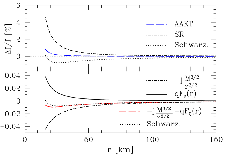
Figure 2: Upper panel: percentage differences between exact numerical values of test particle orbital frequencies, $f_{\rm orb}$, and approximations presented in the text, plotted against the radius of a circular orbit; $\Delta f/f\equiv(f_{orb}-f)/f$, where $f=f^{AAKT}_{orb},f^{sr}_{orb}$, or $f^{Schw.}_{orb}$. Lower panel: values of various terms in Eq. (15) versus orbital radius. For comparison, relative frequency difference in the case of the Schwarzschildian formula is also shown (mass-shedding configuration of DH EOS, details in Appendix).

5 Approximation of the specific orbital energy and angular momentum

We approximate the specific energy and angular momentum of a test particle, in a manner similar to Shibata & Sasaki (1998). As one can see in an example shown in Fig. 2, the difference between the exact orbital frequency and the Schwarzschildian formula is smaller than 1% even for mass-shedding, compact stellar configurations. Near the surface of the star, $f^{Schw.}_{orb}$ is far more accurate than the slow-rotation approximation, and as good as $f^{AAKT}_{orb}$.

Motivated by this result, we aim to provide formulae that are simpler than those of AAKT and which could serve the ambition of being useful in practical calculations. To this aim, we propose to substitute the exact values for the test particle velocity in the Eq. (5) by their approximations of the angular frequency $\Omega$ by $2\pi f^{Schw.}_{orb}$ from Eq. (11), the azimuthal shift component $N^{\phi}$ by the first-order term in the slow-rotation approximation of a frame-dragging term $2GJ/r^{3}c^{2}$, and the metric function $N$ by its Schwarzschildian $c\sqrt{1-r_{s}/r}$:

$$v_{appr.}=(2\pi f^{Schw.}_{orb}-2GJ/r^{3}c^{2})\frac{r}{c\sqrt{1-r_{s}/r}},$$ (16)

where $r\equiv r_{circ}$ for brevity. We then apply $v_{appr.}$, as well as the approximations described above, to Eqs. (6), obtaining $\widetilde{l}^{appr.}$ and $\widetilde{E}^{appr.}$. In Figs. 3, and 4 we compare our approximation with the Schwarzschild, slow-rotation, and AAKT (Eqs. (21) and (26) therein) formulae for $\widetilde{l}$ and $\widetilde{E}$.

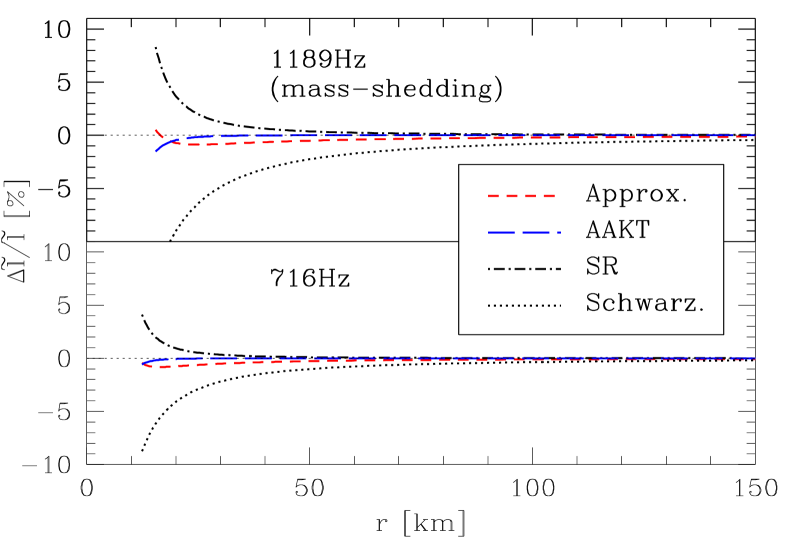
Figure 3: Comparison of specific orbital angular momenta as a function of the radius of the circular orbit. The exact value is denoted by $\widetilde{l}$, while $\widetilde{l}_{\rm a}$ is an approximation of it. The relative deviations (in percent) are $\Delta\widetilde{l}/\widetilde{l}\equiv(\widetilde{l}-\widetilde{l}_{\rm a})/\widetilde{l}$, where $\widetilde{l}_{\rm a}=\widetilde{l}^{appr.},\widetilde{l}^{AAKT},\widetilde{l}^{sr}$ or $\widetilde{l}^{Schw.}$. Results for DH EOS mass-shedding configuration and for the currently-highest pulsar frequency, 716 Hz (details in Appendix).

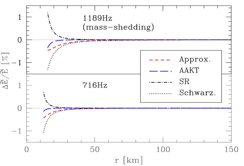
Figure 4: Comparison of specific orbital energies as a function of the radius of the circular orbit. Configurations and notation analogous to Fig. 3.

For different EOSs, masses, and rates of rotation, the behaviour of these deviations is quantitatively and qualitatively similar.

6 Discussion and conclusions

We have performed calculations of stationary configurations of rotating compact stars, for a set of representative EOSs, both polytropic and realistic ones, as well as for the bag models describing the EOSs of hypothetical bare strange quark stars (as in Haensel et al. 2009). In all these cases, we observed quantitatively and qualitatively similar behaviour of the orbital frequency of a test particle moving on a circular orbit in the equatorial plane. In all cases, the value of the orbital frequency was close to that of a test particle in a Schwarzschildian space-time around a point mass (equal to that of the actual compact star), at the properly defined radius. This result is valid for any EOS and for any rotation frequency of the compact star, up to the mass-shedding limit.

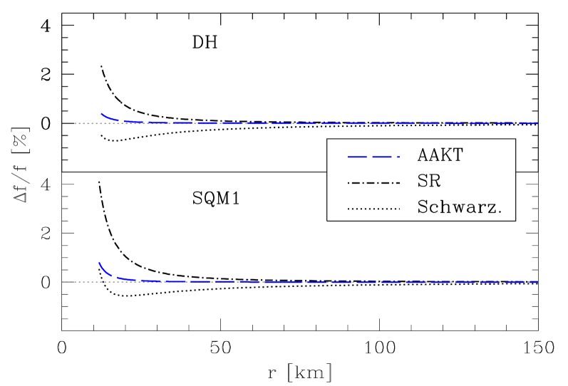
Figure 5: Comparison of orbital frequencies for stellar configurations of DH EOS and bare strange quark star EOS, rotating at 716 Hz. Notations as in Fig. 2, details in Appendix.

We note that the approximations of $\widetilde{l}$ and $\widetilde{E}$, proposed in Sect. 5, reproduce true (numerical) values within about one per cent (being the least accurate in the vicinity of the stellar surface). Their accuracy near the stellar surface decreases to a few percent for rapidly rotating stars with extreme compactnesses ($2GM/Rc^{2}\gtrsim 0.5$), especially in the case of rapidly rotating and oblate bare strange-quark matter stars with large quadrupole moments, but as is shown in Fig. 5 the approximations are acceptable for the currently highest observed spin rate of $716$  Hz. For comparison, Figs. 3 and 4 show the difference in the precision for the DH EOS in the case of the mass-shedding limit and the rotation frequency $716$ Hz.

Overall, our approximations for $\widetilde{l}$ and $\widetilde{E}$ are much better than the slow-rotation approximation, and one does not need to compute the mass-quadrupole moment of the star, the knowledge of which is otherwise crucial in the existing systematic expansions (Berti et al., 2005; Abramowicz et al., 2003). In cases of larger compactness and oblateness, as well as sub-millisecond rotation periods, the approximation from Sect. 5 is in closer agreement with the results of numerical simulations than the formulae of Abramowicz et al. (2003); in Fig. 6, we present an extreme example of a bare quark star spinning at 1300Hz.

The analytic formulae for $f_{\rm orb}(r)$, $\widetilde{l}(r)$, and $\widetilde{E}(r)$ give a very good approximation (typically within a one per cent) of exact values for neutron stars with astrophysically relevant masses, $M\gtrsim 0.5\;{\rm M}_{\odot}$. They are valid for rigidly rotating neutron stars, for rotation rates up to the mass shedding limit, and down to the equator. However, they cannot be used to calculate the properties of the innermost stable circular orbit, because this calculation involves second radial derivatives of metric functions (see, e.g., Cook et al. 1994).

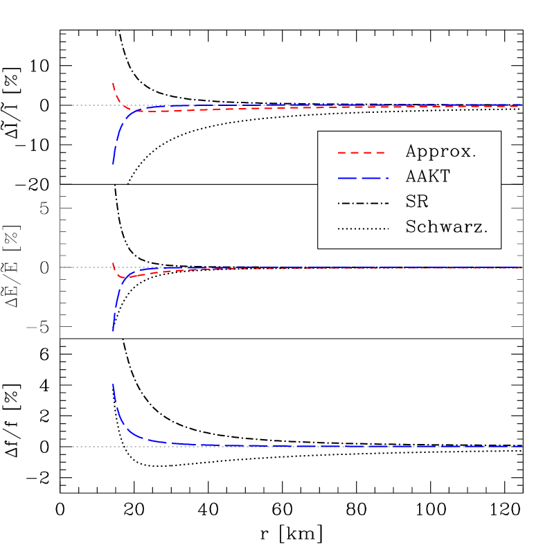
Figure 6: Comparison of $\widetilde{l}$, $\widetilde{E}$, and $f_{orb}$ for $2.2\leavevmode\nobreak\ M_{\odot}$ SQM1 EOS star rotating at 1300 Hz. Notation as in previous figures.

Appendix: Numerical implementation and the EOSs chosen for calculations

The calculations have been performed using the rotstar code from the LORENE library. We use EOSs employed in Haensel et al. (2009):

1. Realistic microphysical EOSs of dense matter. Unless marked otherwise, the figures employ the results for DH EOS of Douchin & Haensel (2001), for a stellar configuration corresponding to a non-rotating star of mass $M=1.43\leavevmode\nobreak\ M_{\odot}$ (central baryon density $n_{b,c}=0.55\leavevmode\nobreak\ {\rm fm^{-3}}$). The mass-shedding configuration has a gravitational mass of $1.8\leavevmode\nobreak\ M_{\odot}$, whereas that rotating at 716 Hz has a mass of $1.52\leavevmode\nobreak\ M_{\odot}$.

2. Bag models of bare strange quark stars. Figs. 5 and 6 show results for SQM1 EOS. The non-rotating counterpart to the stellar configuration presented in Fig. 5 has the gravitational mass of $1.43\leavevmode\nobreak\ M_{\odot}$. The Fig. 6 configuration has a central baryon density of $n_{b,c}=0.63\leavevmode\nobreak\ {\rm fm^{-3}}$, non-rotating gravitational mass of $M=1.7\leavevmode\nobreak\ M_{\odot}$, and compactness $2GM/Rc^{2}=0.47$.

3. Relativistic polytropes. We considered the range $\gamma=1.5-3$ (Tooper, 1965).

References

- Abramowicz et al. (2003) Abramowicz, M. A., et al., 2003, arXiv:gr-qc/0312070 (AAKT)
- Alpar et al. (1982) Alpar, M.A., et al., 1982, Nature, 728
- Altamirano et al. (2010) Altamirano, D., et al., 2010, Astr. Tel., 2565
- Bardeen (1970) Bardeen, J. M., 1970, ApJ 162, 71
- Bardeen (1972) Bardeen, J. M., 1972, ApJ 178, 347
- Bejger et al. (2007) Bejger, M., Haensel, P., Zdunik, J.L., 2007, A&A 464, L49
- Berti et al. (2005) Berti, E., et al., 2005, MNRAS, 358, 923
- Bhattacharya & van den Heuvel (1991) Bhattacharya, D., van den Heuvel, E.P.J., 1991, Phys. Rep. 203, 1
- Cook et al. (1994) Cook, G.B., Shapiro, S.L., Teukolsky, S.A., 1994, ApJ 424, 823
- Douchin & Haensel (2001) Douchin, F., Haensel, P., 2001, A& A, 380, 151
- Haensel et al. (2008) Haensel, P., Zdunik, J.L., Bejger, M., 2008, New Astron. Rev. 51, 785
- Haensel et al. (2009) Haensel, P., et al., 2009 A& A, 502, 605
- Galloway et al. (2009) Galloway, D. K., Lin, J., Chakrabarty, D., Hartman, J. M., 2010 ApJ, 711, L148
- Kerr (1963) Kerr, R .P., 1963, PRL 11, 237
- Kiziltan & Thorsett (2009) Kiziltan, B., Thorsett, S.E., 2009, ApJ 693, L109
- Kluźniak & Wagoner (1985) Kluźniak, W., Wagoner, R.V., 1985, ApJ 297, 548
- Laarakkers & Poisson (1999) Laarakkers, W. G., Poisson, E., ApJ, 512, 282
- Lorimer (2008) Lorimer, D.R., 2008, Living. Rev. Relativity 11, 8. [Online Article]: cited [20 April 2010], http://www.livingreviews.org/lrr-2008-8
- Miller et al. (1998) Miller, M.C., Lamb, F.K., Cook, G.B., 1998, ApJ 509, 793
- Shapiro & Teukolsky (1983) Shapiro, S. L., & Teukolsky, S. A. 1983, Wiley-Interscience
- Shibata & Sasaki (1998) Shibata, M., & Sasaki, M. 1998, PRD 58, 104011
- Tooper (1965) Tooper, R. F., 1965, ApJ 142, 1541
- Zdunik & Gourgoulhon (2001) Zdunik, J.L., Gourgoulhon, E., 2001, PRD 63, 087501
- Zdunik et al. (2002) Zdunik, J.L., Haensel, P., Gourgoulhon, E., 2002, A&A 381, 933