Magnetic scattering of Dirac fermions in topological insulators and graphene
Abstract
We study quantum transport and scattering of massless Dirac fermions by spatially localized static magnetic fields. The employed model describes in a unified manner the effects of orbital magnetic fields, Zeeman and exchange fields in topological insulators, and the pseudo-magnetic fields caused by strain or defects in monolayer graphene. The general scattering theory is formulated, and for radially symmetric fields, the scattering amplitude and the total and transport cross sections are expressed in terms of phase shifts. As applications, we study ring-shaped magnetic fields (including the Aharanov-Bohm geometry) and scattering by magnetic dipoles.
pacs:
73.50.-h, 72.80.Vp, 73.23.-bI Introduction
The recent theoretical prediction and subsequential experimental verification of the conducting surface state existing in a strong topological insulator (TI) has generated a burst of activity, reviewed in Refs. hasan, and qi, . In a TI, strong spin-orbit couplings and band inversion conspire to produce a unique time-reversal invariant topological state different from a conventional band insulator. Using Bi2Se3 as reference TI material, one finds a rather large bulk gap meV, and surface probe experiments have provided strong evidence for the topologically protected gapless surface state.xia The measured spin texture of the surface is well described by two-dimensional (2D) massless Dirac fermions, where the spinor wavefunction has precisely two entries corresponding to physical spin. Under this “relativistic” description, spin and momentum are always perpendicular, and the surface state is stable against the effects of weak disorder and weak interactions due to the underlying topological protection.hasan ; qi Useful insights can then already be obtained from a noninteracting disorder-free description. Massless 2D Dirac fermions are also realized in single carbon monolayers of graphene, for reviews see Refs. review, , castro, and gusynin, . The limit of ballistic transport in this 2D material seems experimentally within reach,andrei ; bolotin and graphene experiments have reported characteristic Dirac fermion signatures, e.g., Klein tunneling.klein1 ; klein2 In most experiments performed so far, correlation effects turned out to be weak, and it is again of interest to examine the single-particle theory in the absence of disorder. In contrast to the TI surface case, the two entries of the spinor wavefunction in graphene correspond to the two atoms in the basis of graphene’s honeycomb lattice. Furthermore, there are four Dirac fermion “flavors” in graphene, due to the physical spin and the (“valley”) orbital degeneracy.castro Another condensed-matter realization of Dirac fermions is given by the quasiparticles in -wave superconductors,dwave but to be specific, we here focus on the surface state in a TI and on monolayer graphene.
The fact that the electronic properties of both these applications correspond to massless 2D Dirac fermions calls for a unified description of their transport properties. In the graphene context, much theoretical effort has been devoted to advancing the scattering theory of Dirac fermions in electrostatic potentials,castro ; novikov in particular for the Coulomb impurity.coulomb In this paper, we instead study the scattering of massless Dirac fermions by a local magnetostatic perturbation. The model, see Eq. (3) below, describes, in a unified manner, the effects of spatially inhomogeneous orbital magnetic fields, exchange-mediated fields due to adjacent ferromagnetic (FM) layers and Zeeman fields in topological insulators, as well as strain- or defect-induced pseudo-magnetic fields in graphene. For the Schrödinger fermions realized in 2D semiconductor electron gases, such perturbations, e.g., magnetically defined barriers, steps, and quantum wells, have been investigated both theoreticallymagbar1 ; magbar2 ; magbar3 ; magbar4 and experimentally.magbarexp ; heinzel The desired magnetic field profiles were generated by deposition of lithographically patterned FM layers on top of the sample. For soft FM materials, one can change the magnetization orientation by weak magnetic fields. Another possibility is to use a type-II superconductor film instead of the FM layer.sup1 ; sup2
Previous theory work on TIs in inhomogeneous magnetic fields has addressed only a few setups. For the transmission of an electron through a magnetic barrier (assumed homogeneous in the transverse direction), as a function of either exchange field or applied bias voltage, Mondal et al.mondal predict an oscillatory behavior or even a complete suppression of the transmission probability, and hence of the conductance. A spin valve geometry with two adjacent magnetic barriers, characterized by non-collinear exchange fields, has also been studied.nagaosa As a model for a classical magnetic impurity, the spin-resolved density of states was calculated for a disc-shaped magnetic field profile.disc1 ; disc2
For graphene, a vector potential perturbation can again be due to external orbital fields, but may also describe the effects of straincastro ; strain1 ; strain2 ; strain3 ; strain4 ; strain5 and dislocations or other topological defects.voz Several theoretical works have addressed aspects of the electronic structure and the transmission properties for Dirac fermions in graphene in the presence of inhomogeneous magnetic fields. The simplest case is encountered for effectively 1D problems with translational invariance in the (say) -direction, e.g., for a magnetic step or a magnetic barrier.ademarti ; ademarti2 ; masir1 For suitable 1D magnetic field profiles, it is possible to have magnetic waveguides (along the -direction),lambert ; ghosh where electron-electron interaction effects play an important role.haus1 Periodic magnetic fields, i.e., 1D magnetic superlattices, have also been addressed.tahir ; luca ; masir2 ; tan For radially symmetric fields, total angular momentum conservation again simplifies the problem and gives an effective 1D theory. This has allowed for studies of quantum dot or antidot geometries,ademarti ; ademarti2 ; kory ; masir3 where true bound states, not affected by Klein tunneling, may exist. In quantum dot setups, interaction effects become important for strong confinement.haus2 When the vector potential corresponds to an infinitely thin solenoid, we encounter an ultra-relativistic Dirac fermion generalization of the celebrated Aharonov-Bohm (AB) calculation.ab ; flux This generalization was discussed before,ruijsenaars ; hagen1 ; hagen2 ; hagen3 ; giacconi ; sakoda and exact results for the transmission amplitude can be deduced. Recent studies have also addressed the current induced by an AB fluxjackiw and the behavior of the conductance when the chemical potential is precisely at the Dirac neutrality point.katsnelson Such an AB conductance can be probed experimentally in ring-shaped graphene devices.ringexp1 ; ringexp2
In this article, we formulate a general scattering theory approach for massless 2D Dirac fermions in the presence of such magnetic perturbations. In Sec. II, we introduce the model and outline its application to graphene and topological insulators. In Sec. III, we formulate the general scattering theory, previously given for electrostatic potentials,novikov for the magnetic case. The scattering amplitude and cross section are specified, and we discuss the Born approximation in Sec. III.1. For the radially symmetric case, total angular momentum conservation allows to express the scattering amplitude in terms of phase shifts for given total angular momentum, see Sec. III.2. In sections IV and V, we present applications of this formalism. First, in Sec. IV, we discuss scattering by a magnetic dipole within the Born approximation. Second, in Sec. V, we consider ring-shaped field profiles. This case also contains the AB solenoid in a certain limit, see Sec. V.2, and we discuss how our phase-shift analysis recovers known results for the AB effect. We also address the scattering resonances appearing due to quasi-bound states in such a ring-shaped magnetic confinement. Finally, some concluding remarks can be found in Sec. VI.
II Dirac fermions in graphene and topological insulators
II.1 Model
In this section, we describe the 2D Dirac fermion model for electronic transport in graphene or the TI surface studied in this work. As perturbations, we first allow for an external static vector potential, with , which is included by minimal coupling and describes orbital magnetic fields and (for graphene) strain-induced pseudo-magnetic fields. In fact, for those applications we have , see below. In addition, for the TI case, we allow for a Zeeman field or for exchange fields caused by nearby ferromagnets, whose components are contained in the field , where prefactors such as the Bohr magneton or the Landé factor are included. With the Pauli matrices and the momentum operator , the single-particle model reads ()
| (1) |
The Fermi velocity in graphene is m/s, while for a TI surface state, a typical valuexia for Bi2Se3 is m/s. The low-energy Hamiltonian in Eq. (1) is valid on energy scales close to the neutrality level (Dirac point), well below the bulk band gap for the TI case and within a window of size eV for graphene. Both the vector potential and the field can now be combined to a vector field
| (2) |
which contains all considered “magnetic” perturbations. Interesting physics also follows in the presence of both and a scalar potential , but we put below.
For the formulation of the scattering theory, it is convenient to employ cylindrical coordinates, and , with unit vectors , and . With Eq. (1) takes the compact form
| (3) | |||||
where the total angular momentum operator is
| (4) |
For the case of azimuthal symmetry, , this is a conserved quantity, , with eigenvalues for half-integer . In Eq. (3) we have put , which is the case for all fields studied below.
Let us now discuss how Eq. (3) relates to the surface states in a strong topological insulator, where the spin direction is tangential to the surface and perpendicular to momentum. For a given two-component spinor wavefunction , the spin () and particle current () density operators arehasan ; qi
| (5) | |||||
i.e., both spin and current are confined to the surface and obey . Under stationary conditions, the continuity equation, , implies the relation
| (6) |
which is linked to the unitarity property of the scattering matrix. Equation (3) then allows to describe the following setups for the TI surface state. First, an orbital magnetic field has only effects when it is oriented perpendicular to the surface, . In cylindrical coordinates, we can then choose some gauge for the vector potential such that
| (7) |
while drops out and is put to zero. Second, to describe the coupling of surface Dirac fermions to an in-plane exchange field , e.g., due to the magnetization of a nearby FM layer, we write with , where we used the spin Pauli matrices in Eq. (5). For a Zeeman field, we can proceed in complete analogy where now denotes the Zeeman field. A Zeeman or exchange field oriented along the direction can open a gap in the spectrum, and here we assume that such fields are not present. While the orbital field breaks time reversal invariance, the Zeeman or exchange fields represent a time-reversal invariant perturbation. Then is determined by the magnetic field itself, and hence is not a gauge field anymore.
Next we turn to graphene, where the Pauli matrices are related to the two triangular sublattices constituting graphene’s honeycomb lattice. We assume that no spin-flip mechanisms are relevant, i.e., physical spin is conserved. We can then focus on one specific Dirac fermion flavor with fixed valley index and spin direction. This excludes exchange or Zeeman fields, i.e., we put and hence for graphene. Note that Zeeman fields in graphene are generally small compared to orbital fields.haus1 Moreover, we consider only smoothly varying vector potentials such that it is indeed sufficient to retain only one point.ademarti Equation (3) can then describe the following cases. First, we may have an orbital magnetic field, precisely as for the TI case. Second, pseudo-magnetic fields generated by strain-induced forces,castro ; strain1 ; strain2 ; strain3 ; strain4 ; strain5 or by various types of defects, e.g., dislocations,voz also correspond to a vector potential, where time reversal invariance implies that has opposite sign at the two points. can then be expressed explicitly in terms of the strain tensor,voz where the resulting pseudo-magnetic field is also oriented along the axis and . In addition, strain causes a scalar potential , which is, however, strongly reduced by screening effects. The combination of orbital and pseudo-magnetic fields may allow to design a valley filter, since the total (orbital plus pseudo-magnetic) fields can differ significantly at both points.valleyfilter
II.2 Multipole expansion
Our scattering theory approach considers magnetic fields [described by in Eq. (3)] that smoothly vary on the scale of a lattice spacing and constitute a local perturbation, i.e., a well-defined cylindrical multipole expansion exists. Furthermore, is assumed throughout. As we show below, for orbital fields we can choose a gauge where . For strain-induced fields, strictly speaking, the problem is not gauge invariant, and we cannot impose gauge conditions. However, in a more narrow sense, a gauge degree of freedom still exists.voz For , with complex-valued coefficients , we then have the multipole expansion
| (8) |
where denotes the total flux in units of the flux quantum .
Let us now address the orbital magnetic field case, , where we can exploit gauge invariance. We start from a more general situation with , expressed as in Eq. (8) with coefficients , and also allow for nonzero coefficients . We now show that one can choose a gauge where and . Indeed, gauge invariance implies that for arbitrary functions , we are free to replace . Using a multipole expansion for with coefficients , an equivalent gauge choice thus follows by the replacement
We then choose the gauge function
In the new gauge, we arrive at Eq. (8) plus the radial component
Using Eq. (7), the orbital field expansion (with ) reads
The term in neither generates flux nor magnetic fields and can be omitted. Magnetic field profiles with arise only in time-dependent settings and will not be studied here. As a consequence, the radial component vanishes, , and we arrive at Eq. (8).
III Scattering theory
For given energy , where throughout, the Dirac equation, with Eq. (3), has scattering solutions that we wish to obtain in the presence of magnetic perturbations of the type in Eq. (8). The solution for follows simply by reversing the sign of the lower spinor component.gusynin We are then looking for a solution consisting, in the asymptotic regime , of a plane wave () propagating along the positive -direction,
| (9) |
plus the scattered outgoing spherical wave,newton
| (10) |
We adopt the same normalization conventions as Novikov.novikov From Eq. (5) we see that the incoming current density is while (for the TI case) the spin density is . Equation (10) defines the scattering amplitude for an outgoing wave deflected under the scattering angle . The resulting scattered current density implies the standard definitions of the differential (), total () and transport () scattering cross sections,novikov ; newton respectively:
| (11) | |||||
The second equality for expresses the 2D optical theorem. When a random distribution of magnetic perturbations is present, the inverse mean free path determining the conductivity is proportional to the transport cross section.abrikosov
III.1 Born approximation
For small perturbation , one can evaluate the scattering amplitude within the first Born approximation.newton Strictly speaking, the long-ranged part in Eq. (8) can not be treated perturbatively, and in this section we assume .
The unperturbed state is the incoming plane wave , Eq. (9). Within lowest-order perturbation theory, the scattered wave obeys
| (12) |
where is the unperturbed Dirac Hamiltonian. Multiplying both sides of Eq. (12) by and noting that in real-space representation, the retarded Green’s function is given by the Hankel function ,novikov ; gradsteyn
The asymptotic large- behavior of the Hankel function (where ) isgradsteyn
| (14) |
which implies that for indeed has the form in Eq. (10). After some algebra, we obtain the scattering amplitude in Born approximation,
| (15) | |||||
For radially symmetric perturbations, , the -integration can be done, and we obtain
with the Bessel function.
III.2 Radially symmetric case
Next, we address the full (beyond Born approximation) scattering solution for radially symmetric perturbations, . In that case, the total angular momentum operator in Eq. (4) is conserved and has eigenvalues with (). We thus expand the spinor wavefunction in terms of angular momentum partial waves
| (17) |
where the Dirac equation yields
| (18) |
The magnetic flux (in units of the flux quantum ) enclosed by a circle of radius around the origin is
| (19) |
where in Eq. (8). The continuity relation (6) must hold for each partial wave separately, and implies
| (20) |
Introducing dimensionless radial coordinates, , a closed equation for the upper component, , follows,
| (21) |
where . The lower component is obtained from
| (22) |
These relations imply a general expression for the scattering amplitude under radially symmetric magnetic perturbations, and thus for the various cross sections in Eq. (11). For , the term in Eq. (8) dominates and the general solution to Eq. (21) is given in terms of Hankel functions,
| (23) |
with complex coefficients and . The lower spinor component then follows from Eq. (22),
| (24) |
The continuity relation (20) implies , i.e., the outgoing wave can differ from a free spherical wave only by a phase shift , which depends on the magnetic perturbation and is determined in Sec. V. Using the Bessel function expansion formula
and the asymptotic behavior of , see Eq. (14), we find
| (25) |
We then obtain the scattering amplitude in terms of phase shifts as for the electrostatic case,novikov
| (26) |
but includes the total flux ,
| (27) |
As a consequence, qualitatively different effects beyond the electrostatic case arise, such as the AB effect. The cross sections in Eq. (11) are then given by
| (28) | |||||
Scattering theory has thus been reduced to the determination of the phase shifts . In the electrostatic case,novikov the phase shifts obey the symmetry relation , implying the absence of backscattering, . In the magnetic case under consideration here, in general this symmetry relation breaks down, and hence backscattering is not suppressed anymore, . This is closely related to the fact that magnetic fields can confine massless Dirac particles.ademarti
IV Magnetic dipoles
As a first application, we analyze the scattering of 2D massless Dirac fermions by a fixed magnetic dipole moment located at position , i.e., at a height above the origin of the 2D plane. In that case no total flux is generated, . The results of this section are obtained under the Born approximation, see Sec. III.1.
IV.1 Perpendicular orientation
First, we consider a dipole moment oriented perpendicular to the layer, , where we have the isotropic (vector potential) perturbation
| (29) |
The Born approximation, see Eq. (III.1), yields the scattering amplitude
| (30) |
and the transport cross section is
| (31) |
Here we define the functions
| (32) |
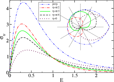
which can be expressed in terms of hypergeometric functions. As shown in Fig. 1, after reaching a maximum around , the transport cross section (31) decreases with increasing energy and approaches zero for . Figure 1 also shows a polar graph for the differential cross section, , at . Evidently, scattering by a dipole oriented along the axis is almost isotropic.
IV.2 Parallel orientation
If the dipole instead points parallel to the layer,
| (33) |
where denotes an angle, we have
| (34) |
i.e., no radial symmetry is present. Using Eq. (15), we now find the scattering amplitude
and thus the transport cross section
| (36) |
where . This cross section depends on the orientation of the dipole even for small energies, . When averaging over (which is equivalent to setting ), we find . The transport cross section (36) has a maximum for an -dependent energy, see Fig. 1, and again approaches zero for . The differential cross section shown in Fig. 1 also reveals a pronounced angular dependence tied to the orientation of the dipole.
IV.3 Bilayer graphene
Let us briefly comment on the results under a quadratic dispersion relation as realized in bilayer graphene.castro Repeating the Born approximation analysis, the scattering amplitude is found to contain an additional factor modifying the above expressions. In fact, we find instead of Eqs. (31) and (36):
with . The quoted expressions hold for the quadratic dispersion relation of bilayer graphene, and coincide with the results for the conventional Schrödinger case. In contrast to the monolayer results for in Eq. (36), the transport cross section (IV.3) carries no -dependence at low energies. The latter is a distinctive feature of 2D massless Dirac fermions. Finally, we note that the results for in Fig. 1 coincide with the bilayer result (when ) for perpendicular orientation.
V Ring-shaped magnetic fields
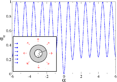
In this section we consider the scattering states for a radially symmetric ring-shaped magnetic field. The scattering setup is schematically sketched in the inset of Fig. 2.
V.1 Infinitesimally thin ring
Let us first study the exactly solvable model of an infinitesimally thin ring of radius around the origin, where follows from Eq. (19) with
| (38) |
where is the Heaviside step function and, as before, is the dimensionless total flux through the ring surface area. For the orbital field case, this implies . With and , the solution to Eq. (21) is
| (39) |
with in Eq. (25). The requirement of continuity of at , together with Eq. (22), leads to two boundary conditions for . With , they read
| (40) |
where again . The coefficient and the phase shift appearing in Eq. (39) then follow from the boundary conditions (40). In particular, when , the phase shift can be determined by evaluation of the logarithmic derivative
where we used the second boundary condition in Eq. (40). As a result, with the Neumann function , we find
| (42) |
while is given by
| (43) |
Equation (42) stays valid beyond the thin-ring limit when a more general form for is used, see Sec. V.3.
V.2 Aharonov-Bohm scattering amplitude
Let us first consider the limit of the above setting, which corresponds to the pure solenoid case. This allows us to study the Aharanov-Bohm (AB) effect for ultra-relativistic Dirac fermions. In order to extract the singular part, we first rewrite in Eq. (23) as
| (44) | |||||
Imposing regularity for as requires the phase shift (27) to be . Correspondingly, for , the scattering amplitude (26) is given by
where , with integer part and non-integer part . Summation of the series in Eq. (V.2) yieldsruijsenaars
Up to the forward scattering () amplitude, Eq. (V.2) reproduces the AB result,ab ; flux ; hagen1 here obtained in terms of scattering phase shifts. Note that the forward scattering -term, missing in the AB calculation,ab naturally appears in our phase shift analysis and is essential for establishing unitarity of the scattering matrix.ruijsenaars ; sakoda
In alternative approaches to obtain for the ideal solenoid, following the original AB method,ab the asymptotics of the exact wavefunction is computed from its integral representation. As a result, the incident wave corresponding to Eq. (9) has an additional phase factor , i.e., one has a multi-valued incoming plane wave. The precise relation between these two approaches has been discussed in several works and is still under debate,ruijsenaars ; hagen1 ; hagen2 ; hagen3 ; giacconi ; sakoda albeit the difference is of little relevance to experimentally observable quantities. In particular, the transport cross section in Eq. (11) does not depend on the forward scattering amplitude at all. We conclude that our approach is able to reproduce the AB effect, , with oscillations as function of the dimensionless flux parameter . In particular, for integer .
V.3 Magnetic ring of finite width
Before discussing concrete results for the scattering amplitude and the transport cross section in the presence of a ring-shaped magnetic field, we now generalize the setup to a finite width, with denoting the inner and outer radii of the ring, cf. the inset of Fig. 2. Again, in Eq. (19) is expressed in terms of a dimensionless flux function . When is a vector potential, the associated magnetic field is taken uniform within the ring region and zero outside; for concreteness, we take . This profile allows for an exact solution, while more general smooth field profiles can be treated within the Wentzel-Kramers-Brillouin (WKB) approximation, see Sec. V.4.
We use dimensionless coordinates ( and ) and flux parameters,
| (47) |
The function then reads with :
| (48) |
For , this reduces to Eq. (38). In particular, in Eq. (48) again denotes the total dimensionless flux.
For given , the components of the Dirac spinor obey Eqs. (21) and (22), with Eq. (48) now determining . The solutions for and are as in Eq. (39),
| (49) |
where and are to be determined, and is given in Eq. (25). For , Eq. (21) can be solved in terms of the confluent hypergeometric functions and ,gradsteyn
| (50) | |||||
The coefficients and , together with and the phase shift in Eq. (49), follow by matching at . Taking into account that is a continuous function of , we have
| (51) |
where the second condition follows by continuity of the lower spinor component . It is convenient to introduce the transfer matrix connecting the solutions at and ,
| (52) |
Explicitly, the transfer matrix for the magnetic ring of finite width is
| (53) |
where we use the abbreviation
and similarly for . We mention in passing that for the infinitesimally thin magnetic ring in Sec. V.1 (where ), the transfer matrix is .
For the finite-width ring, using Eq. (49) the phase shift is then again given by Eq. (42), with and the logarithmic derivative replaced by
| (54) |
With the above expressions, it is straightforward to compute the scattering phases numerically for the finite-width ring geometry. Thereby we obtainfoot the scattering amplitude from Eq. (26) and the transport cross section from Eq. (28).
Numerical results obtained under this approach are shown in Figs. 2 and 3. First, in the main panel of Fig. 2, we show the transport cross section as a function of the total flux . In this example, both radii and were chosen very small, such that scattering by the ring is close to the one by an ideal AB solenoid. As a consequence, we observe the AB oscillations with unit flux period. In contrast to the ideal AB result, a complete suppression of scattering for is observed in the finite-width ring only for , while the maximum value for half-integer is still perfectly realized. In fact, the phase shift analysis in Sec. V.2 shows that a given oscillation period is determined by one specific value in the ideal AB case. For the non-ideal finite-width ring, other total angular momenta also start to contribute, and this mixing effect destroy the perfect constructive interference needed for . On the other hand, the destructive interference responsible for the maxima of at half-integer is more robust since it is dominated by a single value.
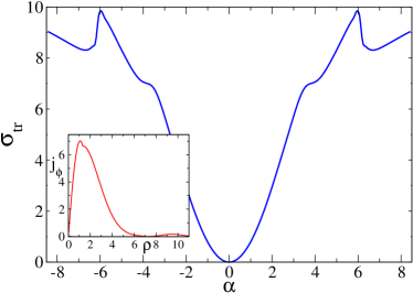
In Fig. 3, we study scattering by a much larger ring. In this case, the AB effect is absent, which can be understood by noting that the Fermi wavelength () of the particle is now smaller than the outer circumference of the ring. Quantum interference of waves surrounding the obstacle in opposite directions is then largely averaged out, and, moreover, the wavefunction can partially penetrate into the ring area. However, a remarkable peak feature at appears now in the transport cross section, see Fig. 3. This feature can be traced to the appearance of a quasi-bound state with at this flux value (for the considered energy), which then causes a scattering resonance, cf. our discussion in Sec. V.4. The inset of Fig. 3 shows the current density profile for precisely this quasi-bound state. While the radial component vanishes, , we find a circularly oriented current, , which is mainly localized inside the ring () and represents a current-carrying bound state. We note that more quasi-bound states appear for larger , causing additional peak features in beyond those shown in Fig. 3.
V.4 Quasi-bound states and scattering resonances
The magnetic confinement built up by the ring-shaped field can generate quasi-bound states, which for become true bound states.ademarti ; ademarti2 The quasi-bound state spectrum then causes resonances in the scattering amplitude when the energy is varied. For given total angular momentum , the corresponding phase shift goes through the value as crosses a resonance level . The corresponding resonance width can be estimated fromnewton
To access these resonances, we first put Eq. (21) into a canonical form with separated kinetic and potential energy terms. The substitution yields
| (55) |
where is an effective potential energy for the radial motion and the lower spinor component is . In this form, Eq. (55) can be treated within the standard WKB approach, which represents an attractive alternative to semiclassical approaches to the Dirac equation as it avoids the appearance of non-Abelian Berry phases.kory ; keppeler ; carmier For a magnetic ring as in Sec. V.3, the effective potential has a hard repulsive core for plus a barrier at larger distances, i.e., a quantum well is formed with classically allowed motion for . The “turning points” here depend on the energy under consideration. For finite , this barrier is of finite width and quasi-bound states within the well region may exist. The classically forbidden region (where is another turning point) then corresponds to tunneling trajectories where the “particle” escapes from the well region. For , the barrier becomes infinitely wide and this escape probability vanishes, i.e., we obtain true bound states in the well region. Using the radial variable , Eq. (55) reads
| (56) | |||
where the modified Bohr-Sommerfeld quantization condition for the complex-valued “energy” ismur
| (57) | |||
with and the Gamma function . The complex resonance values for solving Eq. (57) can be found numerically. Equation (57) is formally exact for the case of a parabolic barrier, but also applies for an arbitrary smooth potential and is expected to remain accuratemur even for small . We now write
For a quasi-bound level with energy , the resonance width is then . Using for , we obtain
| (58) |
where the period of radial motion is
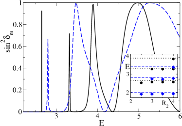
Our numerical results for the partial cross section, , as a function of energy, and the WKB results for the corresponding quasi-bound state energies are shown in Fig. 4. Here we take the field profile as in Sec. V.3.foot2 With increasing (keeping fixed), new quasi-bound energy levels localized in the well region appear, see inset of Fig. 4. Very good agreement with exact quantum calculationsademarti2 for the infinite barrier case () is observed, i.e., these energy levels remain basically unchanged when increasing . The only noticeable deviation from the exact spectrum of Ref. ademarti, is seen for , where the potential creates an infinitely attractive well for . In that case, the WKB approximation becomes questionable in that “steep” region. The main panel in Fig. 4 illustrates the sequence of quasi-bound states present because of the magnetic confinement. The corresponding scattering resonances appear as peaks in the transport cross section when varying energy or the effective flux parameter .
VI Concluding remarks
In this paper, we have studied scattering of massless two-dimensional Dirac fermions by magnetic perturbations of various types. The model is applicable to quantum transport in monolayer graphene and for the surface state of strong topological insulators. The magnetic fields can correspond to orbital or Zeeman fields, strain-induced fields in graphene, or exchange fields generated by ferromagnets.
The full scattering solution was discussed in detail for radially symmetric perturbations, where the scattering amplitude can be expressed in terms of phase shifts in a given total angular momentum channel, and within the Born approximation for the general case. Our approach now allows for a systematic study of the scattering of Dirac fermions on magnetostatic perturbations.
As applications, we have studied scattering by magnetic dipoles within the Born approximation, and fully nonperturbative scattering for the case of ring-shaped magnetic fields. The Born approximation is only valid when the perturbation has zero total flux (). For the magnetic dipole, we have pointed out characteristic angular dependencies in the differential cross section that may allow to unambiguously identify massless Dirac fermions. For the ring-shaped field case, as one increases the lateral size () of the magnetic perturbation, we have a crossover from the Aharonov-Bohm case to a regime dominated by scattering resonances. In the first case, , particle trajectories surround the flux region but essentially do not penetrate it, leading to the oscillatory transport cross section . In the second case, where the particle wavelength is small against the size of the perturbation, , the AB oscillations in are absent. However, now quasi-bound states arise due to the magnetic confinement, causing scattering resonances which show up as peaks in .
To conclude, we hope that these predictions motivate further theoretical work and that they will be tested experimentally in the near future.
Acknowledgements.
We thank A. De Martino for discussions and acknowledge financial support by the DFG Schwerpunktprogramm 1459.References
- (1) M.Z. Hasan and C.L. Kane, arXiv:1002.3895.
- (2) X.-L. Qi and S.-C. Zhang, Physics Today 63, 33 (2010).
- (3) Y. Xia, D. Qian, D. Hsieh, L. Wray, A. Pal, H. Lin, A. Bansil, D. Grauer, Y.S. Hor, R.J. Cava, and M.Z. Hasan, Nature Physics 5, 398 (2009).
- (4) A.K. Geim and K.S. Novoselov, Nat. Mat. 6, 183 (2007).
- (5) A.H. Castro Neto, F. Guinea, N.M.R. Peres, K.S. Novoselov, and A. Geim, Rev. Mod. Phys. 81, 109 (2009).
- (6) V.P. Gusynin, S.G. Shaparov, and J.P. Carbotte, Int. J. Mod. Phys. B 21, 4611 (2007).
- (7) X. Du, I. Skachko, A. Barker, and E.Y. Andrei, Nature Nanotech. 3, 491 (2008).
- (8) K.I. Bolotin, K.J. Sikes, J. Hone, H.L. Stormer, and P. Kim, Phys. Rev. Lett. 101, 096802 (2008).
- (9) N. Stander, B. Huard, and D. Goldhaber-Gordon, Phys. Rev. Lett. 102, 026807 (2009).
- (10) A.F. Young and P. Kim, Nature Physics 5, 222 (2009).
- (11) A. Altland and B.D. Simons, Condensed Matter Field Theory, 2nd edition (Cambridge University Press, 2010).
- (12) D.S. Novikov, Phys. Rev. B 76, 245435 (2007).
- (13) See, for instance, O.V. Gamayun, E.V. Gorbar, and V.P. Gusynin, Phys. Rev. B 80, 165429 (2009), and references therein.
- (14) F.M. Peeters and A. Matulis, Phys. Rev. B 48, 15166 (1993).
- (15) A.M. Matulis, F.M. Peeters, and P. Vasilopoulos, Phys. Rev. Lett. 72, 1518 (1994).
- (16) I.S. Ibrahim and F.M. Peeters, Phys. Rev. B 52, 17321 (1995).
- (17) S.J. Lee, S. Souma, G. Ihm, and K.J. Chang, Phys. Rep. 394, 1 (2004).
- (18) For a review, see: A. Nogaret, J. Phys.: Cond. Matt. 22, 253201 (2010).
- (19) A. Tarasov, S. Hugger, H. Xu, M. Cerchez, T. Heinzel, I.V. Zozoulenko, U. Gasser-Szerer, D. Reuter, and A.D. Wieck, Phys. Rev. Lett. 104, 186801 (2010).
- (20) S.J. Bending, K. von Klitzing, and K. Ploog, Phys. Rev. Lett. 65, 1060 (1990).
- (21) A.K. Geim, S.J. Bending, and I.V. Grigorieva, Phys. Rev. Lett. 69, 2252 (1992).
- (22) S. Mondal, D. Sen, K. Sengupta, and R. Shankar, Phys. Rev. Lett. 104, 046403 (2010); Phys. Rev. B 82, 045120 (2010).
- (23) T. Yokoyama, Y. Tanaka, and N. Nagaosa, Phys. Rev. B 81, 121401(R) (2010).
- (24) Q. Liu, C.-X. Liu, C. Xu, X.-L. Qi, and S.-C. Zhang, Phys. Rev. Lett. 102, 156603 (2009).
- (25) R.R. Biswas and A.V. Balatsky, Phys. Rev. B 81, 233405 (2010).
- (26) A.F. Morpurgo and F. Guinea, Phys. Rev. Lett. 97, 196804 (2006).
- (27) M.M. Fogler, F. Guinea, and M.I. Katsnelson, Phys. Rev. Lett. 101, 226804 (2008).
- (28) V.M. Pereira and A.H. Castro Neto, Phys. Rev. Lett. 103, 046801 (2009).
- (29) W. Bao, F. Miao, Z. Chen, H. Zhang, W. Hang, C. Dames, and C.N. Lau, Nature Nanotech. 4, 562 (2009).
- (30) F. Guinea, M.I. Katsnelson, and A.K. Geim, Nature Phys. 6, 30 (2010).
- (31) M.A.H. Vozmediano, M.I. Katsnelson, and F. Guinea, Physics Reports, in press (2010); see arXiv:1003.5179v2.
- (32) A. De Martino, L. Dell’Anna, and R. Egger, Phys. Rev. Lett. 98, 066802 (2007).
- (33) A. De Martino and R. Egger, Semicond. Sci. Technol. 25, 034006 (2010).
- (34) M. Ramezani Masir, P. Vasilopoulos, A. Matulis, and F.M. Peeters, Phys. Rev. B 77, 235443 (2008).
- (35) L. Oroszlány, P.K. Rakyta, A. Kormányos, C.J. Lambert, and J. Cserti, Phys. Rev. B 77, 081403(R) (2008).
- (36) T.K. Ghosh, A. De Martino, W. Häusler, L. Dell’Anna, and R. Egger, Phys. Rev. B 77, 081404(R) (2008).
- (37) W. Häusler, A. De Martino, T.K. Ghosh, and R. Egger, Phys. Rev. B 78, 165402 (2008).
- (38) M. Tahir and K. Sabeeh, Phys. Rev. B 77, 195421 (2008).
- (39) L. Dell’Anna and A. De Martino, Phys. Rev. B 79, 045420 (2009).
- (40) M. Ramezani Masir, P. Vasilopoulos, and F.M. Peeters, New. J. Phys. 11, 095009 (2009).
- (41) L.Z. Tan, C.-H. Park, and S.G. Louie, Phys. Rev. B 81, 195426 (2010).
- (42) A. Kormányos, P. Rakyta, L. Oroszlány, and J. Cserti, Phys. Rev. B 78, 045430 (2008).
- (43) M. Ramezani Masir, A. Matulis and F.M. Peeters, Phys. Rev. B 79, 155451 (2009).
- (44) W. Häusler and R. Egger, Phys. Rev. B 80, 161402(R) (2009).
- (45) Y. Aharonov and D. Bohm, Phys. Rev. 115, 485 (1959).
- (46) S. Olariu and I.I. Popescu, Rev. Mod. Phys. 57, 339 (1985).
- (47) S.N.M. Ruijsenaars, Ann. Phys. (N.Y.) 146, 1 (1983).
- (48) C.R. Hagen, Phys. Rev. Lett. 64, 503 (1990).
- (49) C.R. Hagen, Phys. Rev. D 41, 2015 (1990).
- (50) C.R. Hagen, Phys. Rev. D 52, 2466 (1995).
- (51) P. Giacconi, F. Maltoni, and R. Soldati, Phys. Rev. D 53, 952 (1996).
- (52) S. Sakoda and M. Omote, J. Math. Phys. 38, 716 (1997).
- (53) R. Jackiw, A.I. Milstein, S.Y. Pi, and I.S. Terekhov, Phys. Rev. B 80, 033413 (2009).
- (54) M.I. Katsnelson, EPL 89, 17001 (2010).
- (55) P. Recher, B. Trauzettel, A. Rycerz, Ya.M. Blanter, C.W.J. Beenakker, and A.F. Morpurgo, Phys. Rev. B 76, 235404 (2007).
- (56) S. Russo, J.B. Oostinga, D. Wehenkel, H.B. Heersche, S.S. Sobhani, L.M.K. Vandersypen, and A.F. Morpurgo, Phys. Rev B 77, 085413 (2008).
- (57) T. Fujita, M.B.A. Jalil, and S.G. Tan, arXiv:1005.5088.
- (58) R.G. Newton, Scattering theory of waves and particles, 2nd edition (Springer, New York, 1982).
- (59) A.A. Abrikosov, L.P. Gorkov, and I.E. Dzyaloshinski, Methods of quantum field theory in statistical physics (Prentice Hall, Inc., Eaglewood Cliffs, New Jersey, 1963).
- (60) I.S. Gradshteyn and I.M. Ryzhik, Table of Integrals, Series and Products (Academic Press, New York, 1980).
- (61) In the numerical evaluation, we sum over all angular momentum states (with ). Scattering phases with very large are difficult to compute reliably yet average out in practice.
- (62) J. Bolte and S. Keppeler, Ann. Phys. (N.Y.) 274, 125 (1999).
- (63) P. Carmier and D. Ullmo, Phys. Rev. B 77, 245413 (2008).
- (64) V.D. Mur and V.S. Popov, JETP Lett. 51, 563 (1990).
- (65) In order to avoid artefacts caused by treating sharp boundaries within the WKB approach, we have used a smoothening of the field steps.