All Optical Measurement Proposed for the Photovoltaic Hall Effect

Abstract

We propose an all optical way to measure the recently proposed gphotovoltaic Hall effect h, i.e., a DC Hall effect induced by a circularly polarized light in the absence of static magnetic fields. For this, we have calculated the Faraday rotation angle induced by the photovoltaic Hall effect with the Kubo formula extended for photovoltaic optical response in the presence of strong AC electric fields treated with the Floquet formalism. We also point out the possibility of observing the effect in three-dimensional graphite, and more generally in multi-band systems such as materials described by the dp-model.

1 Introduction

There are increasing fascinations with new types of Hall effect besides the quantum Hall effect in magnetic fields, where a notable example is the spin Hall effect in topological insulators. We have previously proposed, as another new type of Hall effect, the gphotovoltaic Hall effect h, which should take place when we shine a circularly polarized light to graphene[1]. The effect is interesting since this Hall effect occurs in the absence of uniform magnetic fields. Physically, the photovoltaic Hall current originates from the Aharonov-Anandan phase (a non-adiabatic generalization of the geometric (Berry) phase) that an electron acquires during its circular motion around the Dirac points in k-space in an AC field, and bears, in this sense, a topological origin similar to the quantum Hall effect. However, unlike the quantum Hall effect, the photovoltaic Hall conductivity is in general not quantized.

We have originally proposed an experimental setup to measure the photovoltaic Hall current through the gate electrodes attached to the sample. In the present report we propose a second, all-optical setup, which employs the Faraday rotation as in the optical Hall effect discussed in refs. [2, 3], which becomes here non-linear optical measurements, since this is a “pump-probe” type experiment, where one optically probes the Hall effect that is induced in a system pumped by a circularly polarized light from a continous laser source. This effect should grow with the intensity of the applied circularly polarized light. We also point out the possibility of observing the effect not only in graphene, but also in three-dimensional graphite, and more generally in multi-band systems such as materials described by the $dp$-lattice.

2 Kubo-formula extended for optical responses in a strong background light

So let us first propose a method to measure the photovoltaic Hall effect with non-linear optical measurements. The experimental setup is schematically displayed in Fig.1(a), where the sample is subject to a strong circularly polarized light with strength $F$ and frequency (photon energy) $\Omega$. The strong external AC field changes the properties of the electronic state and the photo-induced band, or the Floquet band to be more precise, can acquire a non-trivial topological nature. This was discussed in ref. [1] as an emergence of the photovoltaic Berry’s curvature. Optical repsonse can be drastically change in the presence of the photovoltaic Berry’s curvature, which we show here to be captured through an optical Faraday (or Kerr) rotation measurement. Our starting point to calculate the optical response is the Floquet expression for the Kubo formula extendend to incorporate photovoltaic transports [1],

$$\sigma_{ab}(\mbox{\boldmath$A$}_{\rm ac})=i\int\frac{d\mbox{\boldmath$k$}}{(2\pi)^{d}}\sum_{\alpha,\beta\neq\alpha}\frac{[f_{\beta}(\mbox{\boldmath$k$})-f_{\alpha}(\mbox{\boldmath$k$})]}{\varepsilon_{\beta}(\mbox{\boldmath$k$})-\varepsilon_{\alpha}(\mbox{\boldmath$k$})}\frac{\langle\langle\Phi_{\alpha}(\mbox{\boldmath$k$})|J_{b}|\Phi_{\beta}(\mbox{\boldmath$k$})\rangle\rangle\langle\langle\Phi_{\beta}(\mbox{\boldmath$k$})|J_{a}|\Phi_{\alpha}(\mbox{\boldmath$k$})\rangle\rangle}{\varepsilon_{\beta}(\mbox{\boldmath$k$})-\varepsilon_{\alpha}(\mbox{\boldmath$k$})+i\eta}$$ (1)

with $a,b=x$ or $y$. The DC expression can be extended to AC responses, which reads

$$\sigma_{xy}(\omega;\mbox{\boldmath$A$}_{\rm ac})=-i\int\frac{d\mbox{\boldmath$k$}}{(2\pi)^{d}}\sum_{\alpha,\beta\neq\alpha}\frac{f_{\beta}(\mbox{\boldmath$k$})}{\varepsilon_{\beta}(\mbox{\boldmath$k$})-\varepsilon_{\alpha}(\mbox{\boldmath$k$})}$$ (2)

$$\hskip 22.76228pt\times\left[\frac{\langle\langle\Phi_{\alpha}(\mbox{\boldmath$k$})|J_{x}|\Phi_{\beta}(\mbox{\boldmath$k$})\rangle\rangle\langle\langle\Phi_{\beta}(\mbox{\boldmath$k$})|J_{y}|\Phi_{\alpha}(\mbox{\boldmath$k$})\rangle\rangle}{\varepsilon_{\beta}(\mbox{\boldmath$k$})-\varepsilon_{\alpha}(\mbox{\boldmath$k$})+\omega+i\eta}-\frac{\langle\langle\Phi_{\alpha}(\mbox{\boldmath$k$})|J_{y}|\Phi_{\beta}(\mbox{\boldmath$k$})\rangle\rangle\langle\langle\Phi_{\beta}(\mbox{\boldmath$k$})|J_{x}|\Phi_{\alpha}(\mbox{\boldmath$k$})\rangle\rangle}{\varepsilon_{\beta}(\mbox{\boldmath$k$})-\varepsilon_{\alpha}(\mbox{\boldmath$k$})-\omega+i\eta}\right],$$

for the $xy$-component and

$$\mbox{Re}\;\sigma_{xx}(\omega;\mbox{\boldmath$A$}_{\rm ac})=\frac{\pi}{\omega}\int\frac{d\mbox{\boldmath$k$}}{(2\pi)^{d}}\sum_{\alpha<\beta}[f_{\alpha}(\mbox{\boldmath$k$})-f_{\beta}(\mbox{\boldmath$k$})]|\langle\langle\Phi_{\beta}(\mbox{\boldmath$k$})|J_{x}|\Phi_{\alpha}(\mbox{\boldmath$k$})\rangle\rangle|^{2}\delta(\varepsilon_{\beta}(\mbox{\boldmath$k$})-\varepsilon_{\alpha}(\mbox{\boldmath$k$})-\omega)$$ (3)

for the $xx$-component. Here $|\Phi_{\alpha}(t)\rangle$ is the $\alpha$-th Floquet state, the double brakets includes a time average, $f_{\alpha}(\mbox{\boldmath$k$})$ the non-equilibrium distribution (occupation fraction) of the $\alpha$-th Floquet state, and $\eta$ a positive infinitesimal. Strictly speaking, we must take into account the effect of relaxation (phonons, electrodes, etc.) to determine the non-equilibrium distribution function as a detailed balanced state with photo-absorbtion, photo-emission and the relaxations. Here we assume for simplicity that the non-equilibrium distribution function is given by

$$f_{\alpha}(\mbox{\boldmath$k$})=\sum_{i}|\langle\langle\psi_{i}|\Phi_{\alpha}(\mbox{\boldmath$k$})\rangle\rangle|^{2}f_{\rm FD}(E_{i},\mu;\beta_{\rm eff}),$$ (4)

where $f_{\rm FD}(E_{i},\mu;\beta_{\rm eff})=1/[\exp(\beta_{\rm eff}(E_{i}-\mu))+1]$ is the equilibrium Fermi-Dirac distribution with an effective inverse temperature $\beta_{\rm eff}$. This corresponds to employing a sudden approximation. A proper treatment of the relaxation can be done using the Keldysh Green’s function as in ref. [1].

2.1 Experimental feasibility

In discussing the experimental feasibility, we can start from the relation between the induced conductivities $\sigma_{xx}(\omega),\sigma_{xy}(\omega)$ and the Faraday-rotation angle $\Theta_{H}$ [2],

$$\Theta_{H} = \frac{1}{2}\mbox{arg}\left[\frac{n_{0}+n_{s}+(\sigma_{xx}+i\sigma_{xy})/(c\varepsilon_{0})}{n_{0}+n_{s}+(\sigma_{xx}-i\sigma_{xy})/(c\varepsilon_{0})}\right]$$ (5)

$$= \frac{1}{(n_{0}+n_{s})c\varepsilon_{0}}\sigma_{xy}(\omega)\sim(\sigma_{xy}\;\mbox{in units of }\frac{e^{2}}{h})\;\times\;7\;\mbox{mrad}.$$ (6)

This gives an estimate for the experimental precision demanded to observe the photovoltaic Hall effect through optical measurements. For example, in Fig.1 below, we estimate the photo-induced response $\sigma_{xy}(\omega;\mbox{\boldmath$A$})$ for a single-layered graphene to be around $0.2$. This corresponds to a Faraday-rotation angle of $\Theta_{H}\sim 0.2\times 7=1.4\;\mbox{mrad}$.

3 Photovoltaic optical response

3.1 Single-layer graphene

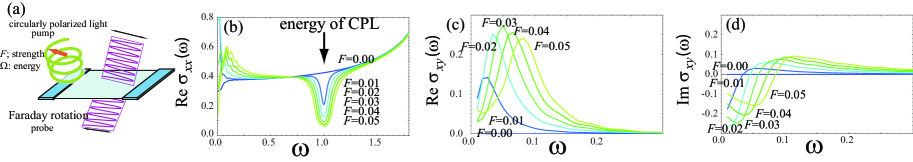
Figure 1: (a) Schematic, all-optical experimental setup to measure the photovoltaic Hall effect via non-linear optical responses. (b)(c)(d) Photovoltaic optical response in the honeycomb lattice (single-layer graphene). The optical absorption spectrum $\mbox{Re}\sigma_{xx}(\omega;\mbox{\boldmath$A$})$ (b) and the “photovoltaic optical Hall coefficient” $\sigma_{xy}(\omega;\mbox{\boldmath$A$})$ (c,d) are plotted for various values of strength $F$ of the circularly polarized light. Note the different scales between (b) and (c,d). Here the energy of light is fixed to $\Omega=1.0$ in units of the hopping integral ($t\sim 3$ eV for graphene), and the effective inverse temperature $\beta_{\rm eff}=100$.

Using the extended Kubo formula (eqns. (2),(3)), we calculate the non-linear optical response in the presence of a strong circularly-polarized light in the honeycomb lattice. The optical absorption spectrum in Fig. 1 (b) exhibits the following: (i) At the energy of the circularly-polarized light (CPL), there is a dip in the absorption ($\sigma_{xx}(\omega)$, which is an analogue of hole burning. (ii) Near the DC limit ($\omega\to 0$), as one increases the field strength, the absorption first increases due to photo-carriers but then decreases. The decrease is due to the opening of a photo-induced gap at the Dirac point as discussed in ref. [1]. The real and imaginary parts of the photovoltaic optical Hall coefficient are plotted in Fig. 1 (c,d), which grow in a low-frequency region. The peak position of the real part shifts to higher frequency as the strength of the CPL is increased. This is important, since the experimental detection is easier for higher photon energies.

3.2 Multi-layer graphene

Photovoltaic Hall effect is not restricted to systems having a Dirac cone as in the single-layer graphene. To show this, we calculate the photovoltaic optical response in bilayer graphene (see [4] for notation and refs) described by the Hamiltonian,

$$H=\left(\begin{array}[]{cccc}0&k_{x}-ik_{y}&t_{p}&0\\ k_{x}+ik_{y}&0&0&0\\ t_{p}&0&0&k_{x}+ik_{y}\\ 0&0&k_{x}-ik_{y}&0\end{array}\right).$$ (11)

We plot the photovoltaic optical response in Fig. 2 for this effective model. The basic features are similar to those in the monolayer graphene. The result suggests the possibility of observing photovoiltaic Hall effect in mulilayer graphene and graphite, since one can block-diagonalize the Hamiltonian for a multilayer system into sub-blocks of single and bi-layer graphene components as was shown in ref. [5].

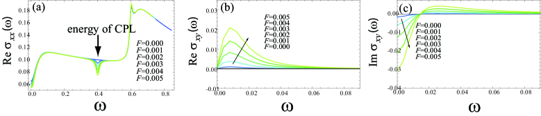
Figure 2: Photovoltaic optical response in a bilayer graphene for $\Omega=1.0,\;t_{p}=0.6$ with different scales between (a) and (b,c). Note that the input field is an order of magnitude weaker than in Fig.1.

4 Photovoltaic Berry’s curvature in the $dp$-lattice

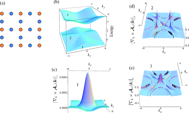
Figure 3: (a) $dp$-lattice. (b) The band dispersion in the $dp$ model. (c)(d)(e) Photovoltaic Berry’s curvature in the three bands (top d-band (c), and middle (d), bottom (e) p-bands) for $t_{dp}=0.4,\;\varepsilon_{d}-\varepsilon_{p}=4,\;F=0.01,\;\Omega=3.$.

We finally explore the possibility of more generally observing the photovoltaic Hall effect in materials other than graphene/graphite. For a typical multiband model, we consider here the $dp$-lattice, which is a well-studied lattice in connection with the high-Tc cuprates[7]. Here we neglect the electron-electron interaction to consentrate on the one-particle properties. The Hamiltonian is given by

$$H = \left(\begin{array}[]{ccc}\varepsilon_{d}-\varepsilon_{p}&-2t\sin\frac{k_{x}}{2}&-2t\sin\frac{k_{y}}{2}\\ -2t\sin\frac{k_{x}}{2}&0&4t_{dp}\sin\frac{k_{x}}{2}\sin\frac{k_{y}}{2}\\ -2t\sin\frac{k_{y}}{2}&4t_{dp}\sin\frac{k_{x}}{2}\sin\frac{k_{y}}{2}&0\end{array}\right),$$ (15)

where $\varepsilon_{d}-\varepsilon_{p}$ is the potential difference between the $d$ and $p$ bands. The photovoltaic DC Hall conductivity is expressed as Berry’s curvature as [1, 6]

$$\sigma_{xy}(\mbox{\boldmath$A$}_{\rm ac})=e^{2}\int\frac{d\mbox{\boldmath$k$}}{(2\pi)^{d}}\sum_{\alpha}f_{\alpha}(\mbox{\boldmath$k$})\left[\nabla_{\mbox{\boldmath$k$}}\times\mbox{\boldmath$\mathcal{A}$}_{\alpha}(\mbox{\boldmath$k$})\right]_{z},$$ (16)

in terms of a gauge field $\mbox{\boldmath$\mathcal{A}$}_{\alpha}(\mbox{\boldmath$k$})\equiv-i\langle\langle\Phi_{\alpha}(\mbox{\boldmath$k$})|\nabla_{\mbox{\boldmath$k$}}|\Phi_{\alpha}(\mbox{\boldmath$k$})\rangle\rangle$. Note that this expression reduces to the TKNN formula [8] in the adiabatic limit.

The band dispersion of the $dp$-lattice is shown in Fig. 3 (b) and the photovoltaic Berry’s curvature for each band is plotted in (c)-(e). A peak in Berry’s curvature emerges at the center of the Brilliouin zone in the $d$-band, while the curvatue has complex structures in the $p$-bands. This is because the two $p$-bands intersect with each other, for which the ac field induces a band mixing, while the $d$-band is separated from the $p$-bands with the separation larger than the photon energy $\Omega$ considered in the figure.

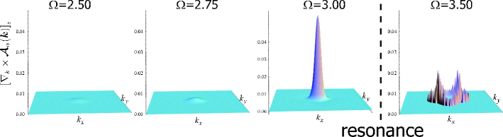
Figure 4: Photovoltaic Berry’s curvature in the $d$-band of the $dp$-lattice for severa values of thel photon energy $\Omega$ for $t_{dp}=0.4,\;\varepsilon_{d}-\varepsilon_{p}=4,\;F=0.1$.

Now, a natural question is: Is there a difference between a system with a band gap as in the $dp$-lattice when compared to a system with a massless Dirac cone as in graphene? In order to clarify this, we have calculated the photovoltaic Berry’s curvature for several values of $\Omega$ in Fig. 4. When $\Omega$ is smaller than the gap, the photovoltaic Berry curvature increases as the value of $\Omega$ approaches the band gap. When $\Omega$ exceeds the gap, when a direct photo-transition becomes possible, the Berry’s curvature changes into a concentric form with a negative part (not apparent in the figure). In the massless Dirac case, both the cone-like contribution and the concentric form coexist[1, 6], while in the $dp$-lattice they appear separately. Another important obervation is that the magnitude of the photovoltaic Hall effect becomes large in multiband systems when $\Omega$ is slightly below the band gap, whereas in the massless Dirac case small $\Omega$ is better.

To conclude, we have studied the possibility of observing the photovoltaic Hall effect in an all-optical fashion. We have also shown that the effect is not restricted to lattices with a massless Dirac cone but is a universal phenomenon in multi-band systems. HA has been supported in part by a Grant-in-Aid for Scientific Research No.20340098 from JSPS, TO by a Grant-in-Aid for Young Scientists (B) from MEXT and by Scientific Research on Priority Area “New Frontier of Materials Science Opened by Molecular Degrees of Freedom”.

References

References

- [1] T. Oka, and H. Aoki, Phys. Rev. B 79, 081406 (R) (2009); ibid 79, 169901(E) (2009).
- [2] T. Morimoto, Y. Hatsugai, and H. Aoki, Phys. Rev. Lett. 103, 116803 (2009).
- [3] Y. Ikebe, T. Morimoto, R. Masutomi, T. Okamoto, H. Aoki, and R. Shimano, Phys. Rev. Lett. 104, 256802 (2010).
- [4] A. H. Castro Neto, F. Guinea, N. M. R. Peres, K. S. Novoselov, and A. K. Geim, Rev. Mod. Phys. 81, 109 (2009).
- [5] M. Koshino and T. Ando, Phys. Rev. B 76, 085425 (2007).
- [6] T. Oka and H. Aoki, J. Phys.: Conf. Ser. 200, 062017 (2010).
- [7] F. C. Zhang and T. M. Rice, Phys. Rev. B 37, 3759 (1988).
- [8] D. J. Thouless, M. Kohmoto, M. P. Nightingale, and M. den Nijs, Phys. Rev. Lett. 49, 405 (1982).